Article

Turbo Channel Covariance Conversion in Massive MIMO Frequency Division Duplex Systems

by
Zhuying Yu
,
Shengsong Luo
and
Chongbin Xu
*
Department of Communication Science and Engineering, Fudan University, Shanghai 200433, China
*
Author to whom correspondence should be addressed.
Electronics 2025, 14(8), 1490; https://doi.org/10.3390/electronics14081490
Submission received: 9 March 2025 / Revised: 2 April 2025 / Accepted: 5 April 2025 / Published: 8 April 2025

Abstract

:
Estimating the downlink (DL) channel covariance matrix (CCM) is crucial for beamforming and capacity optimization in massive MIMO frequency division duplexing (FDD) systems, yet it poses significant challenges due to the lack of direct channel reciprocity. To address this issue, a turbo channel covariance conversion (Turbo-CCC) algorithm is proposed to enhance estimation accuracy and robustness by utilizing the angular power spectrum (APS) reciprocity. Specifically, based on the electromagnetic wave propagation characteristics, we model the APS as multikernel functions. On this basis, we then develop the Turbo-CCC algorithm by integrating the orthogonal approximate message passing (OAMP) algorithm and the multikernel adaptive filtering (MKAF) algorithm based on a Bayesian framework. The OAMP module estimates the APS from the uplink (UL) CCM regardless of its structural characteristics, whereas the MKAF module refines the APS estimation by leveraging its structural characteristics. These two modules operate iteratively, progressively improving the accuracy of the DL CCM estimation. Simulation results demonstrate that the proposed algorithm noticeably enhances the estimation performance and exhibits strong adaptability to diverse APS distributions and propagation environments, offering a novel approach for the DL CCM estimation in massive MIMO FDD systems.

1. Introduction

With the rapid advancement of wireless communication technologies, the demand for higher spectral efficiency and improved communication reliability has surged. Massive multi-input multi-output (MIMO) systems have emerged as a key solution to meet these demands [1]. However, the performance of MIMO systems heavily relies on the accurate acquisition of channel state information (CSI) at the base station (BS) [2,3]. To enhance the accuracy and efficiency of CSI acquisition, various approaches have been explored. Among them, message passing algorithms have been widely adopted due to their ability to iteratively refine CSI estimates by exploiting prior information and leveraging the inherent sparsity of the channel [4,5,6]. Furthermore, to address the computational challenges associated with high-dimensional CSI estimation, various complexity reduction techniques have been proposed [7,8,9], significantly reducing the estimation overhead while maintaining satisfactory accuracy.
However, instantaneous CSI is influenced by multipath effects and noise, leading to rapid variations. In contrast, statistical CSI, based on the long-term statistical characteristics of the channel, exhibits higher stability, making it more suitable for practical communication systems [10]. So one key aspect of CSI estimation is the accurate characterization of the channel covariance matrices (CCMs), which describe the statistical properties of the channel.
For time division duplex (TDD) systems, the downlink (DL) CCM can be obtained efficiently via channel reciprocity [11]. However, for frequency division duplex (FDD) systems, the uplink (UL) and DL channels operate on different frequency bands, so there is no inherent reciprocity [12]. This discrepancy poses a significant challenge to estimate the DL CCM from the UL CCM.
To overcome this challenge, several techniques have been proposed in the literature to enable the estimation of the DL CCM in massive MIMO FDD systems [13,14,15]. Specifically, by observing that the difference between UL and DL spatio-temporal correlation lies solely in a dilation proportional to the ratio between UL and DL carrier frequency, a cubic spline interpolation method was proposed in [13] to estimate the DL CCM from the UL CCM in MIMO FDD systems. Based on the mapping function between the UL and DL, a covariance variational auto-encoder network (CVENet) was proposed in [16], which extracts the UL CCM into a latent distribution space and estimates DL CCM from samples in this space, achieving improved estimation accuracy.
Additionally, several measurement campaigns have found that, since the UL and DL share the same physical environment, the angular power spectrum (APS) is frequency invariant [17,18]. This is referred to as APS reciprocity, which can be exploited to acquire the DL CCM by estimating the APS from the UL CCM, followed by using the estimated APS to obtain the DL CCM. However, estimating the APS from the UL CCM is an ill-posed problem, which may lead to significant deviations in the reconstructed DL CCM.
To address this issue, we can leverage the characteristics of the APS, such as sparsity and smoothness. Specifically, by fully exploiting the sparsity of the APS, compressive sensing (CS) was proposed as an effective approach to estimate the DL CCM from the UL CCM in [19]. The proposed CS-based approach efficiently addresses the challenge of estimating DL CCM in FDD systems.
Another notable method was discussed in [20], which provides a robust solution for DL CCM acquisition by exploiting the APS reciprocity and employing efficient projection methods in an infinite-dimensional Hilbert space. Based on the minimum 2 norm constraint of the APS, the paper proposed the Projection Onto a Linear Variety (PLV) algorithm, which outperforms current state-of-the-art solutions in terms of accuracy and flexibility.
Despite the progress made in this area, challenges remain in improving the accuracy and robustness of DL CCM estimation in FDD systems. In particular, the signal experiences multiple reflections, scattering, and diffraction, creating various propagation paths and different angles of arrival, which leads to a complex structure of the APS [21,22]. Furthermore, the inaccuracy of UL CCM exacerbates the challenges. To address these challenges, one direction is to continue studying the structural characteristics of the APS. In practical environments, the APS exhibits a concentrated distribution in certain specific directions, resembling multiple peaks. Therefore, it can be approximated by several Gaussian functions [23,24]. We can leverage this structural characteristic of the APS to enhance the performance of existing methods.
In this paper, we focus on the challenging problem of DL CCM estimation in massive MIMO FDD systerms. Based on the sparsity and structural characteristics of the APS, we propose a novel algorithm by integrating the orthogonal approximate message passing (OAMP) algorithm and the multikernel adaptive filtering (MKAF) algorithm under a Bayesian framework. The main contributions of the paper are outlined as follows:
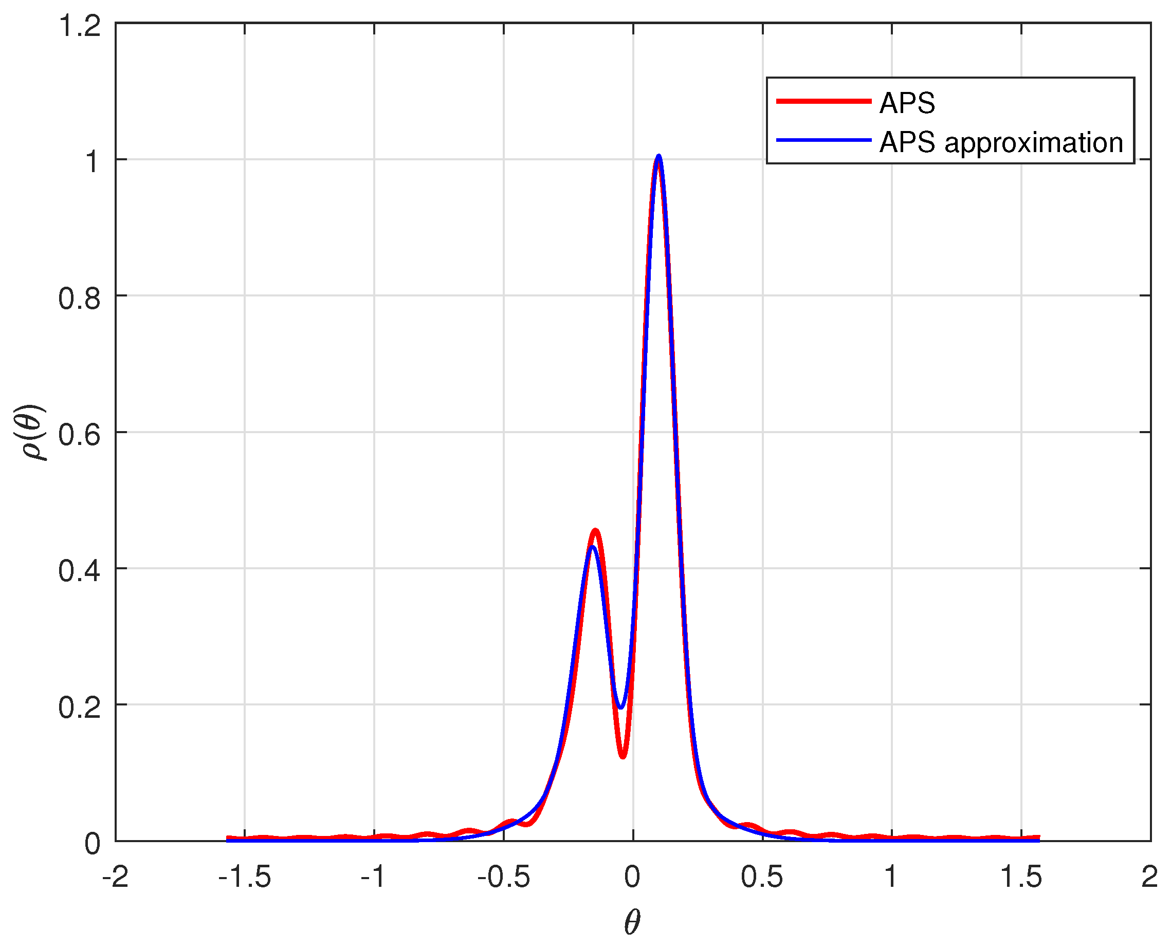
  • In a multipath propagation environment, the signal undergoes multiple reflections, scattering, and diffraction, resulting in different propagation paths and arrival angles. The APS exhibits a concentrated distribution in these directions, resembling multiple peaks. Therefore, we model the APS using multiple Gaussian functions, with each Gaussian function representing the signal energy distribution in a specific direction.
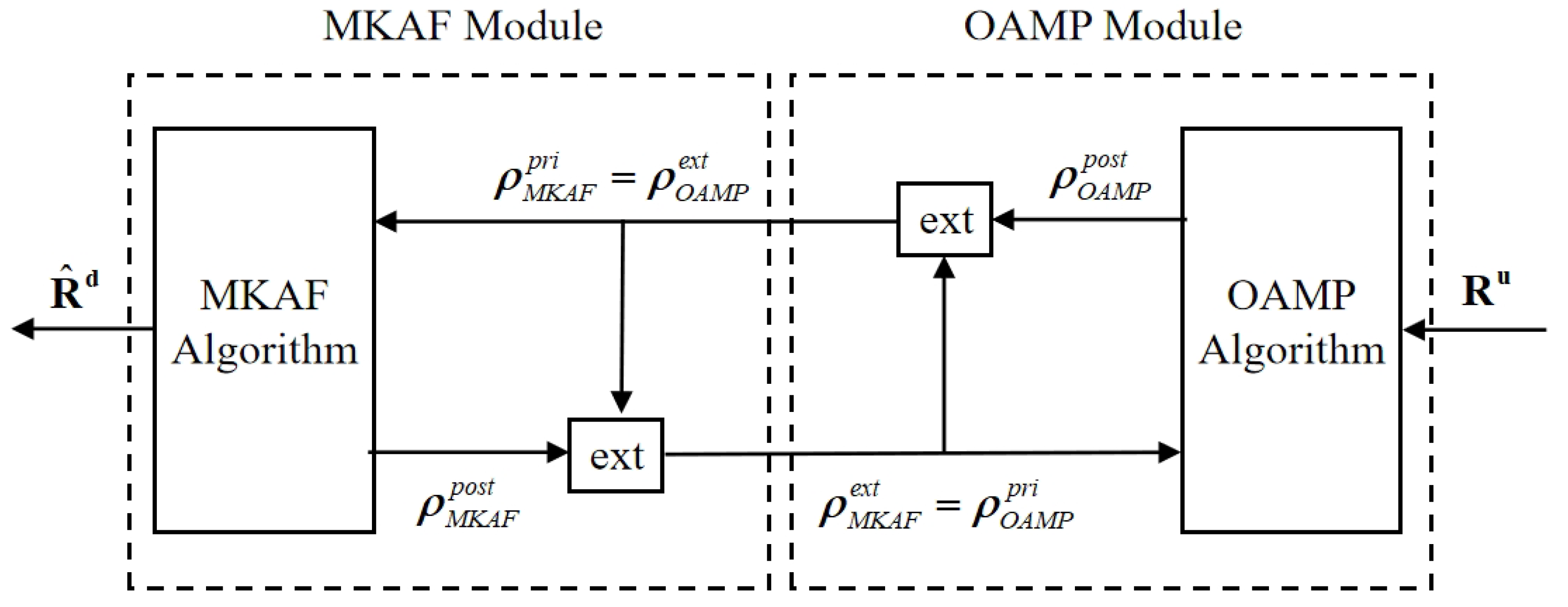
  • Based on the APS reciprocity, we propose a turbo channel covariance conversion (Turbo-CCC) algorithm composed of two modules: the OAMP module and the MKAF module. The OAMP module estimates the APS based on the UL CCM, while the MKAF module extracts relevant information from the structural characteristics of the APS to refine the APS estimation. These two modules operate iteratively, progressively improving the accuracy of the DL CCM estimation.
  • Our numerical results demonstrate that the proposed algorithm achieves higher accuracy and robustness in DL CCM estimation compared to conventional methods. It is applicable to most practical scenarios, making it an effective solution for DL CCM estimation in FDD massive MIMO systems.
The rest of this paper is organized as follows. Section 2 outlines system models and formulates the corresponding DL CCM estimation problem. Section 3 develops the proposed algorithm. Our numerical results are provided in Section 4. Finally, the advantages and potentials of the proposed algorithm are discussed in Section 5.
Notation: The scalars are denoted by letters in normal fonts. The vectors and the matrices are denoted by bold lowercase letters and bold capital letters, respectively. The operators ( · ) T , ( · ) * and ( · ) H denote transpose, conjugate, and conjugate transpose, respectively. We use · to denote the modulus of a vector/matrix and · F is the Frobenius norm. vec ( A ) denotes the operator that stacks column-wise the elements of a matrix A into a column vector. N ( x ; μ , τ ) denotes the probability distribution function (pdf) for a variable x following a Gaussian distribution with mean μ and variance τ ; CN ( x ; μ , τ ) denotes the pdf for a variable x following a complex Gaussian distribution with mean μ and variance τ .

2. System Model and Problem Formulation

In this section, we present the system model and formulate the problem addressed in this paper.

2.1. System Model

We consider a MIMO wireless communication system where a BS equipped with N antennas communicates with user equipment (UE) that has a single antenna. We denote the channel between the BS and user at time t Z as h [ t ] C N × 1 . Due to the physical environment and antenna array configuration, the channel exhibits spatial correlation. The spatial characteristics are captured by the CCM at the BS and UE. We mainly focus on the transmit and receive CCMs obtained at the BS, which are defined as [25]:
R d : = E h d [ t ] h d [ t ] H , R u : = E h u [ t ] h u [ t ] H ,
where h d [ t ] and h u [ t ] denote the the DL channel and UL channel, respectively. R d and R u denote the the DL CCM and UL CCM, respectively. The covariance matrices describe the second-order statistics of the channel and depend on the APS distributions in the environment. For a uniform linear array (ULA) at the BS, the relationship between CCM and APS is expressed as [26]:
R f = Ω ρ f ( θ ) a f ( θ ) a f ( θ ) H d θ , f { u , d } ,
where u and d denote the UL and DL frequency, respectively. ρ f ( θ ) is the APS. According to the APS reciprocity, we have ρ u ( θ ) = ρ d ( θ ) = ρ ( θ ) , where ρ : Ω R + characterizes the received or transmitted power in a specific physical direction θ Ω [ π , π ] . a f ( θ ) : Ω C N × 1 are antenna array responses dependent on frequency, which is defined as
a f ( θ ) = 1 N 1 e j 2 π d λ f sin θ e j 2 π d λ f ( N 1 ) sin θ T , f { u , d } ,
where d R denotes the inter-antenna spacing and λ R denotes the carrier wavelength. Due to the inherent symmetry of ULA, which cannot distinguish between a direction of arrival (DoA) θ and its reciprocal θ + π , the APS is typically restricted to the range θ Ω [ π / 2 , π / 2 ] . This assumption is further justified by practical considerations, as real systems often employ similar or even more constrained sectorization of the cell, effectively limiting the relevant spatial directions.

2.2. Problem Formulation

In this paper, we focus on DL CCM acquisition in massive MIMO FDD systems. This problem can be formulated as follows:
max p ( R d | R u ) , s . t . R f = Ω ρ ( θ ) a f ( θ ) a f ( θ ) H d θ , f { u , d } , a f ( θ ) = 1 N 1 e j 2 π d λ f sin θ e j 2 π d λ f ( N 1 ) sin θ T , f { u , d } .
One possible way to solve this problem is to utilize the APS reciprocity, but estimating the APS from the UL CCM is an ill-posed problem, which can be addressed by leveraging the structural characteristics of the APS. Given the complexity of the APS structure, we propose the Turbo-CCC algorithm to address this problem in the following section.

3. Proposed Algorithm

In this section, we first construct an extended probability model of the considered problem by considering the structural characteristics of the APS, based on which the structure of the Turbo-CCC algorithm is developed. We then present a detailed description of the proposed algorithm.

3.1. Extended Probability Model and Algorithm Structure

In communication systems, the APS often exhibits smooth variations due to the natural propagation environment, where the angles of arrival typically cluster around a few dominant directions. The Gaussian function is known for its ability to efficiently represent smooth distributions, making it an ideal candidate for modeling APS, as shown in Figure 1. Therefore, we can model the APS as follows [27]:
ρ ( θ ) = j = 1 J h j exp θ c j ξ j 2 + n ( θ ) ,
where J > 0 is the number of Gaussian functions, h j R is the coefficient, c j R and ξ j R are the mean and variance of Gaussian functions, respectively. n ( θ ) represents the noise. We define γ : = { ( h j , ξ j , c j ) j = 1 , , J } as the set of the parameters.
We need to jointly estimate the APS ρ ( θ ) and the parameters of Gaussian functions γ . The corresponding extended probabilistic model can be written as
p ( R d , R u , ρ ( θ ) , γ ) = ( a ) p ( R d | R u , ρ ( θ ) , γ ) p ( R u ρ ( θ ) , γ ) · p ( ρ ( θ ) γ ) p ( γ ) = ( b ) p ( R d | ρ ( θ ) ) p ( R u ρ ( θ ) ) p ( ρ ( θ ) γ ) p ( γ ) ,
where the step ( a ) is due to the Bayesian formula and step ( b ) is due to the Markov property between the Bayes formula and the variables.
Based on (6), we propose a Turbo-CCC algorithm consisting of two modules. Specifically, the OAMP module corresponds to the conditional probability p ( R u ρ ( θ ) ) and the MKAF module corresponds to the conditional probability p ( ρ ( θ ) γ ) . The structure of the algorithm is shown in Figure 2.
The functions of the two modules are summarized as follows.
  • OAMP Module: The OAMP module leverages the UL CCM and the prior information m ρ ( M K A F O A M P ) ( ρ ) fed back from the MKAF module to estimate the APS from UL CCM. Subsequently, it passes the messages m ρ ( O A M P M K A F ) ( ρ ) to the MKAF module. We formulate the APS estimation problem as a CS problem, which will be addressed using the OAMP algorithm. For details, see Section 3.2.
  • MKAF Module: This module first utilizes the messages m ρ ( O A M P M K A F ) ( ρ ) to estimate the parameters of Gaussian functions γ , which is solved based on the MKAF algorithm. Subsequently, this module derives the extrinsic information of the APS based on Bayesian inference, which is defined as m ρ ( M K A F O A M P ) ( ρ ) , and then passes it to the OAMP module for iterative refinement. In the final iteration, DL CCM estimation is generated based on the posterior mean of the APS. For details, see Section 3.3.

3.2. Orthogonal Approximate Message Passing Module

To leverage the APS reciprocity for channel covariance conversion, the first step is to estimate the APS from the UL CCM based on (2). Directly handling the integral form poses challenges. Hence, we reformulate the equation to better suit the problem under investigation, as elaborated below.
For practical implementation, the domain of θ is discretized into M angles θ m m = 1 M , leading to the approximation of (2) when f = u :
R u = m = 1 M ρ θ m a u θ m a u θ m H .
Let A u = a u θ 1 , a u θ 2 , , a u θ M represent the array response matrix for the discretized angles. The covariance matrix can then be expressed in a compact form as:
R u = A u diag ( ρ ) A u , H ,
where ρ = [ ρ ( θ 1 ) , ρ ( θ 2 ) , , ρ ( θ M ) ] T is the APS vector. diag ( ρ ) represents a diagonal matrix whose main diagonal elements are given by the vector ρ while all off-diagonal elements are zero.
To facilitate analysis, the UL CCM is vectorized. By applying the formula vec ( ABC ) = ( C T A ) · vec ( B ) to the right-hand side of (8), the vectorized UL CCM is given by:
r u = vec ( R u ) = A 1 u ρ ,
where
A 1 u = A u * A u = a u θ 1 * a u ( θ 1 ) , , a u θ M * a u ( θ M ) R N 2 × M ,
where ⊗ denotes the Kronecker product, and A u * is the complex conjugate of A u .
Considering the noise, (9) can be expressed as:
r u = A 1 u ρ + n ,
where n is additive white Gaussian noise with a mean of 0 and a variance of σ 2 .
Thus far, we have formulated the problem as (11), which is a CS problem that can be addressed using various approaches. We utilize the OAMP algorithm due to its low computational complexity, fast convergence, and strong robustness compared with other CS algorithms.
OAMP alternates between two key steps: a linear estimation (LE) and a nonlinear estimation (NLE).
LE : s ( t ) = ρ ^ ( t ) + W t ( r u A 1 u ρ ^ ( t ) ) ,
NLE : ρ ^ ( t + 1 ) = η ˜ t ( s ( t ) ) .
Define the error terms:
q ( t ) = ρ ^ ( t ) ρ , h ( t ) = s ( t ) ρ .
Substituting (13) into (12), we can obtain
LE : h ( t ) = ( I W t A 1 u ) q ( t ) + W t n ,
NLE : q ( t + 1 ) = η ˜ t ( ρ + h ( t ) ) ρ .
Moreover, we define error-related parameters:
v ^ ( t ) = lim M 1 M q ( t ) 2 2 ,
τ t 2 = lim M 1 M h ( t ) 2 2 .
Recall that OAMP distinguishes itself from standard approximate message passing (AMP) primarily through two critical features; η t is divergence-free and W t is de-correlated. To meet these requirements, we proceed with the following steps.
For the first feature, we first present the following signal estimation problem.
S = X + τ t Z ,
where X P ρ ( ρ ) and Z N ( 0 , 1 ) are random variables and are independent of each other.
η ˜ t is divergence-free if
E { η ˜ t ( S ) } = 0 .
A divergence-free denoiser η ˜ t can be constructed as
η ˜ t ( s ( t ) ) = C η t ( s ( t ) ) s ( t ) η t ( s ( t ) ) ,
where C is an arbitrary constant and η t ( · ) is an arbitrary function. · denotes the average of a vector.
For another feature, we will say the LE (or W t ) is a de-correlated one if tr ( I W t A 1 u ) = 0 . We can construct W t to satisfy tr ( I W t A 1 u ) = 0 as follows:
W t = M tr ( W ^ t A 1 u ) W ^ t .
We choose to use linear minimum mean square error (LMMSE) de-correlated matrix as given in [28]:
W ^ t = A 1 u , T A 1 u A 1 u , T + σ 2 v ^ ( t ) I 1 .
By restricting W t to be de-correlated while ensuring η ˜ t is divergence-free, the orthogonality between the input and output error terms for both LE and NLE can be maintained. We follow [28] in referring to this algorithm as “orthogonal AMP”.
According to Lemma 1 in [28], the optimal η ˜ t that minimizes the MSE E { ( η ˜ t ( X + τ t Z ) X ) 2 } at the final iteration is given by:
η ˜ t * ( s ( t ) ) = C * η t mmse ( s ( t ) ) v ^ mmse ( t ) τ t 2 s ( t ) ,
where
C * = τ t 2 τ t 2 v ^ mmse ( t ) ,
η t mmse ( s i ( t ) ) = E { ρ | s i ( t ) , τ t 2 } ,
v ^ mmse ( t ) = 1 M i = 1 M Var { ρ | s i ( t ) , τ t 2 } .
The expectation in (24) can be obtained from
E { ρ | s i ( t ) } = ρ P ρ ( ρ ) N ( ρ ; s i ( t ) , τ t 2 ) d ρ P ρ ( ρ ) N ( ρ ; s i ( t ) , τ t 2 ) d ρ ,
where P ρ ( ρ ) is the prior information m ρ ( M K A F O A M P ) ( ρ ) fed back from the MKAF module.
Then
v ^ ( t ) = lim M 1 M q ( t ) 2 = E Z , X C * η t mmse ( X + τ t Z ) v ^ mmse ( t ) ( X + τ t Z ) τ t 2 X 2 = ( a ) E Z , X τ t 2 τ t 2 v ^ mmse ( t ) η t mmse X + τ t Z X τ t v ^ mmse ( t ) τ t 2 v ^ mmse ( t ) Z 2 = ( b ) τ t 2 τ t 2 v ^ mmse ( t ) 2 v ^ mmse ( t ) + τ t v ^ mmse ( t ) τ t 2 v ^ mmse ( t ) 2 = 1 v ^ mmse ( t ) 1 τ t 2 1 ,
where the step ( a ) is due to the definition of C * in (23) and step ( b ) is due to v ^ mmse ( t ) = E Z , X η t mmse X + τ t Z X 2 .
Then, applying (23) and (27) to (22), we derive
ρ ^ ( t + 1 ) = η ˜ t ( s ( t ) ) = v ^ ( t ) η t mmse ( s ( t ) ) v ^ mmse ( t ) s ( t ) τ t 2 ,
where τ t 2 is given as follows [28]:
τ t 2 = lim M 1 M h ( t ) 2 = 1 M tr ( I W t A 1 u ) ( I W t A 1 u ) T v ^ ( t ) + 1 M tr ( W t W t T ) σ 2 .
Based on the above derivation, the OAMP algorithm is presented in Algorithm 1. We can obtain ρ ^ through iteration, and then pass the message m ρ ( O A M P M K A F ) ( ρ ) = N ( ρ ; ρ ^ , v ^ ) to the MKAF Module.
Algorithm 1 OAMP algorithm.
Input:  r u ,   A 1 u ,   σ 2 ,   and   P ( ρ ) .
Initialization:  ρ ^ ( 1 ) = 0 ,   v ^ ( 1 ) = 1 .
   for  t = 1 : T
       W ^ t = A 1 u , T A 1 u A 1 u , T + σ 2 v ^ ( t ) I 1
       W t = M tr ( W ^ t A 1 u ) W ^ t
       τ t 2 = 1 M tr ( I W t A 1 u ) ( I W t A 1 u ) T v ^ ( t ) + 1 M tr ( W t W t T ) σ 2
       s ( t ) = ρ ^ ( t ) + W t r u A 1 u ρ ^ ( t )
       ρ ^ mmse ( t + 1 ) = η t mmse s ( t ) , τ t 2
       v ^ mmse ( t ) = 1 M i = 1 M Var ρ s i ( t ) , τ t 2
       v ^ ( t + 1 ) = 1 v ^ mmse ( t ) 1 τ t 2 1
       ρ ^ ( t + 1 ) = v ^ ( t ) η t mmse ( s ( t ) ) v ^ mmse ( t ) s ( t ) τ t 2
   end
Output: APS estimate ρ ^ ( T ) .

3.3. Multikernel Adaptive Filtering Module

To leverage the structural characteristics of the APS, we model the APS using Gaussian functions. The messages obtained from the OAMP module m ρ ( O A M P M K A F ) ( ρ ) = ρ ^ are used to estimate the parameters of the Gaussian functions { h j } , { c j } , { ξ j } , which can be expressed as
ρ ^ ( θ ) = j = 1 J h j exp θ c j ξ j 2 + n ( θ ) .
Existing methods for estimating these parameters include least squares (LS), EM, MKAF, and so on. In our approach, we choose the MKAF algorithm due to its high flexibility and adaptability, which are particularly suited for real-time processing and enable the algorithm to effectively capture the complex structural characteristics of the APS. However, the MKAF algorithm yields hard information, so we further process the results using Bayesian inference to obtain soft information that can be used for iteration.
Let us define a dictionary as the following set of functions:
D n : = { κ ( · , c j , n ; ξ j , n ) j = 1 , , J n } , n N ,
where n denotes the n-th iteration. κ ( θ , c j , n ; ξ j , n ) : = exp θ c j , n ξ j , n 2 is the Gaussian kernel. Then, the filter is formulated as
φ n ( θ ) : = j = 1 J n h j , n κ ( θ , c j , n ; ξ j , n ) , j = 1 J n .
γ n : = { ( h j , n , ξ j , n , c j , n ) j = 1 , , J n } are defined as the set of parameters. The parameters are determined by minimizing the cost function, as shown below:
argmin γ n L n ( γ n ) : = ρ ^ n φ ( J n ) ( θ n ) 2 + λ Ω n ( h n ) ,
where h n = [ h 1 , n , h 2 , n , , h J n , n ] R J n . Ω n ( h ) : = j = 1 J n h j , n reduces the dictionary’s size by enforcing sparsity on the h n . λ is the parameter of regularization.
The process of updating the parameters can be divided into two steps. The first step is to screen suitable variances. We adopt a strategy of initializing variances with multiple values ξ init ( 1 ) ξ init ( 2 ) ξ init ( Q ) > 0 . To prevent rapid expansion of the dictionary size, a multiscale screening method is applied, i.e., evaluate κ ( · , θ n ; ξ init ( 1 ) ) ,…, κ ( · , θ n ; ξ init ( Q ) ) one by one to check if they meet the error and coherence conditions, and add the first one κ ( · , θ n ; ξ init ( q ) ) that satisfies the conditions to the dictionary. ( 0 , ξ init ( q ) , θ n ) is the initial parameters. The error condition is defined as
| ρ ^ n φ n ( θ n ) | > ϵ ( q ) , q Q ,
where ϵ ( 1 ) ϵ ( 2 ) ϵ ( Q ) > 0 is a predefined constant. The coherence condition is given by
coherence ( q ) : = max j = 1 , , J n κ ( θ n , c j ; ξ init ( q ) ) δ ( q ) , q Q ,
where δ ( q ) ( 0 , 1 ) is a predefined threshold.
Another step is to update the kernel parameters γ n : = { ( h j , n , ξ j , n , c j , n ) j = 1 , , J n } . We first utilize the adaptive proximal forward backward splitting (APFBS) algorithm [29] to minimize (33) with respect to h n . The proximity operator prox λ Ω : R J n R J n is defined as
prox λ Ω n ( x ) = argmin y R J n λ Ω n ( y ) + 1 2 x y 2 .
We can update h n as
h n + 1 : = T prox λ Ω n h n + μ ( h ) ( ρ ^ n h n T κ n ) κ n ,
where μ ( h ) [ 0 , 2 ] is the stepsize parameter. The operator T is used to eliminate zero components.
Then, we utilize the mirror descent method [30] to update the variances ξ j , n , which is expressed as
ξ j , n + 1 = argmin ξ R + ξ , L n ( γ n ) ξ j + B ϕ ( ξ | | ξ j , n ) μ j , n ( ξ ) ,
where B ϕ ( ξ | | ξ j , n ) : = ϕ ( ξ ) ϕ ( ξ j , n ) ϕ ( ξ j , n ) , ξ ξ j , n is a Bregman divergence with ϕ ( x ) : = x log x x , x > 0 , and μ j , n ( ξ ) = ξ j , n μ ( η ) , μ ( η ) > 0 is the stepsize parameter. L n ( γ n ) ξ j is given by
L n ( γ n ) ξ j = 2 e n h j , n θ n c j , n 2 κ ( θ n , c j , n ; ξ j , n ) ξ j , n 2 .
Taking the derivative of the right side of (38) and setting it to zero, we obtain
ξ j , n + 1 = exp log ( ξ j , n ) μ j , n ( ξ ) L n ( γ n ) ξ j .
Finally, we update the means c j , n using the stochastic gradient descent algorithm [31], which is formulated as
c j , n + 1 = c j , n μ ( c ) L n ( γ n ) c j ,
where μ ( c ) > 0 is the stepsize parameter, and L n ( γ n ) c j is defined as
L n ( γ n ) c j = 4 e n h j , n κ ( θ n , c j , n ; ξ j , n ) ( θ n c j , n ) ξ j , n .
Next, we update the estimation of ρ using the messages passed from the previous procedures. The messages m ρ ( O A M P M K A F ) ( ρ ) = N ( ρ ; ρ ^ , v ^ ) from the OAMP module are considered as prior information. We sample around the coefficients { h j } , { c j } , { ξ j } to obtain a set of L samples for ρ . Therefore, the likelihood information can be expressed as 1 L l = 1 L δ ( ρ ρ l ) . The posterior probability of ρ can be formulated as
p p o s t ( ρ ) p p r i o r ( ρ ) · p l i k e h o o d ( ρ ) = N ( ρ ; ρ ^ , v ^ ) · 1 L l = 1 L δ ( ρ ρ l ) .
The exact computation of this distribution is usually challenging, so we approximate it with a Gaussian distribution N ( ρ ; u ρ , v ρ ) . u ρ and v ρ can be formulated as
u ρ = ρ p p o s t ( ρ ) d ρ p p o s t ( ρ ) d ρ = ρ N ( ρ ; ρ ^ , v ^ ) · l = 1 L δ ( ρ ρ l ) d ρ N ( ρ ; ρ ^ , v ^ ) · l = 1 L δ ( ρ ρ l ) d ρ = l = 1 L ρ l N ( ρ l ; ρ ^ , v ^ ) l = 1 L N ( ρ l ; ρ ^ , v ^ ) ,
v ρ = mean ( diag ( R ρ ) ) ,
where mean ( · ) denotes the average of the vector, and diag ( · ) denotes extracting the diagonal elements of the matrix. R ρ is given as follows:
R ρ = ( ρ u ρ ) ( ρ u ρ ) T p p o s t ( ρ ) d ρ p p o s t ( ρ ) d ρ = ( ρ u ρ ) ( ρ u ρ ) T N ( ρ ; ρ ^ , v ^ ) · l = 1 L δ ( ρ ρ l ) d ρ N ( ρ ; ρ ^ , v ^ ) · l = 1 L δ ( ρ ρ l ) d ρ = l = 1 L ( ρ l u ρ ) ( ρ l u ρ ) T N ( ρ l ; ρ ^ , v ^ ) l = 1 L N ( ρ l ; ρ ^ , v ^ ) .
Extrinsic information of ρ can be then calculated as
m ρ ( M K A F O A M P ) ( ρ ) = p p o s t ( ρ ) / N ( ρ ; ρ ^ , v ^ ) .
The messages m ρ ( M K A F O A M P ) ( ρ ) are passed to the OAMP module to start the next iteration.
Based on the above derivation, the MKAF algorithm is presented in Algorithm 2.
Algorithm 2 MKAF algorithm.
Input:  θ m , ρ ^ ( θ m ) .
    for  m = 1 : M  do
        Screen suitable variances by (34) and (35).
        Update the kernel parameters γ m by (37), (38) and (41).
    end for
    Update the extrinsic information of ρ by (43)–(47);
Output: Extrinsic information m ρ ( M K A F O A M P ) ( ρ ) .

3.4. Overall Algorithm

Based on the procedure described in Section 3.1, Section 3.2 and Section 3.3, our proposed algorithm is summarized in Algorithm  3. The OAMP module and the MKAF module are iteratively executed in a loop until the following convergence condition is satisfied:
| MSE ( ρ ) ( l ) MSE ( ρ ) ( l 1 ) | < ϵ ,
where MSE ( ρ ) ( l ) : = E [ ρ ρ ^ F 2 / ρ F 2 ] denotes the mean square error (MSE) of APS estimation at iteration l, and ϵ is an empirically determined convergence threshold. In the large system limit ( M , N ) , the dynamics of the OAMP algorithm can be characterized through state evolution (SE). Due to the limited number of antennas in our work, it is difficult to provide a rigorous convergence analysis. The damping mechanism [32] is applied to improve convergence and stability.
Finally, the estimated ρ ^ is output from the MKAF module, based on which the estimated DL CCM R ^ d is obtained.
Algorithm 3 Turbo-CCC algorithm.
Input:  R u , A 1 u , σ 2 .
Repeat
    //OAMP Module
    for  t = 1 : T  do
        Update APS estimate ρ ^ by Algorithm 1.
    end for
    Pass message m ρ ( O A M P M K A F ) ( ρ ) to MKAF module.
    //MKAF Module
    for  m = 1 : M  do
        Update extrinsic information m ρ ( M K A F O A M P ) ( ρ ) by Algorithm 2.
    end for
    Pass message m ρ ( M K A F O A M P ) ( ρ ) to OAMP module.
Until: The convergence condition (48) is satisfied.
Generate DL CCM estimate R ^ d based on the posterior mean ρ ^ = u ρ from MKAF module in the final iteration by (2).
Output: DL CCM estimate R ^ d .
The computational complexity analysis of the proposed Turbo-CCC algorithm can be derived as follows. First, as a key component of the algorithm, the OAMP module exhibits a complexity of O ( T N M ) , where T denotes the number of iterations. This complexity primarily stems from matrix operations during the iterative process. Second, the MKAF module demonstrates a complexity of O ( M J n ) , where J n represents the number of Gaussian kernels, with its computational overhead mainly arising from the calculation of Gaussian kernel parameters. Consequently, the overall algorithmic complexity can be expressed as O ( t ( T N + J n ) M ) , where t denotes the total number of iterations. In practical applications, the trade-off between computational complexity and performance can be balanced by adjusting the number of iterations through ϵ .

4. Numerical Results

In this section, we present a series of simulations to validate the performance of the proposed algorithm.

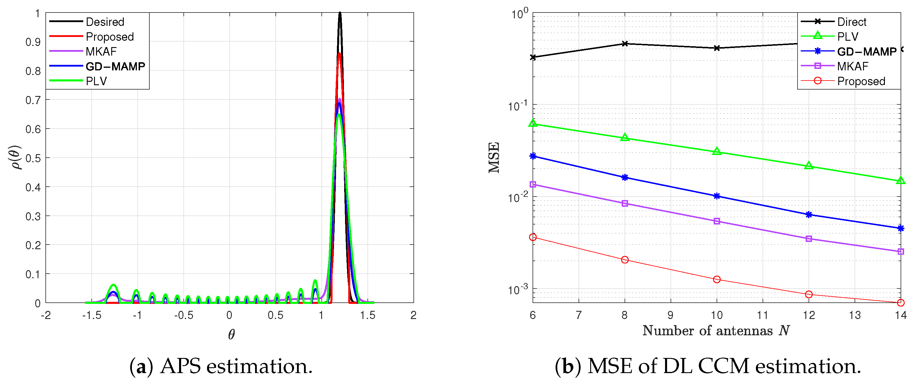
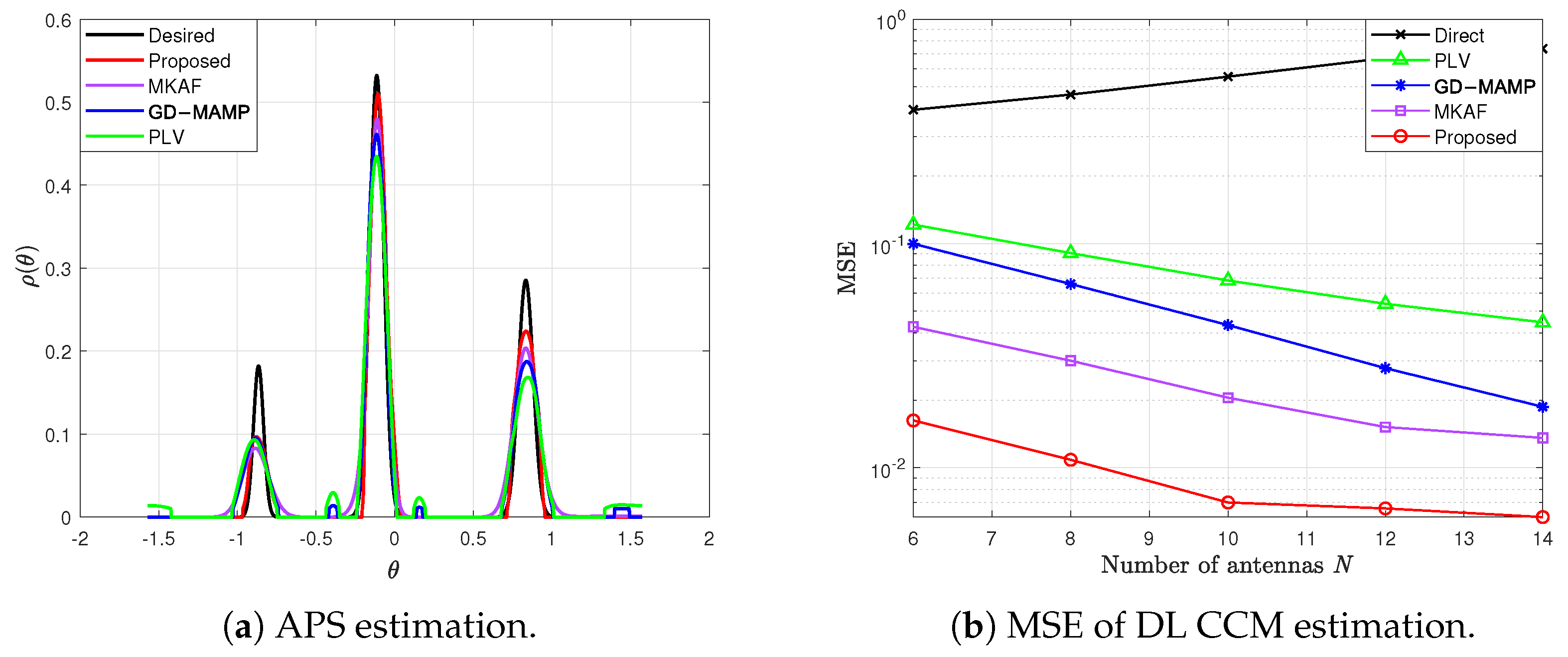
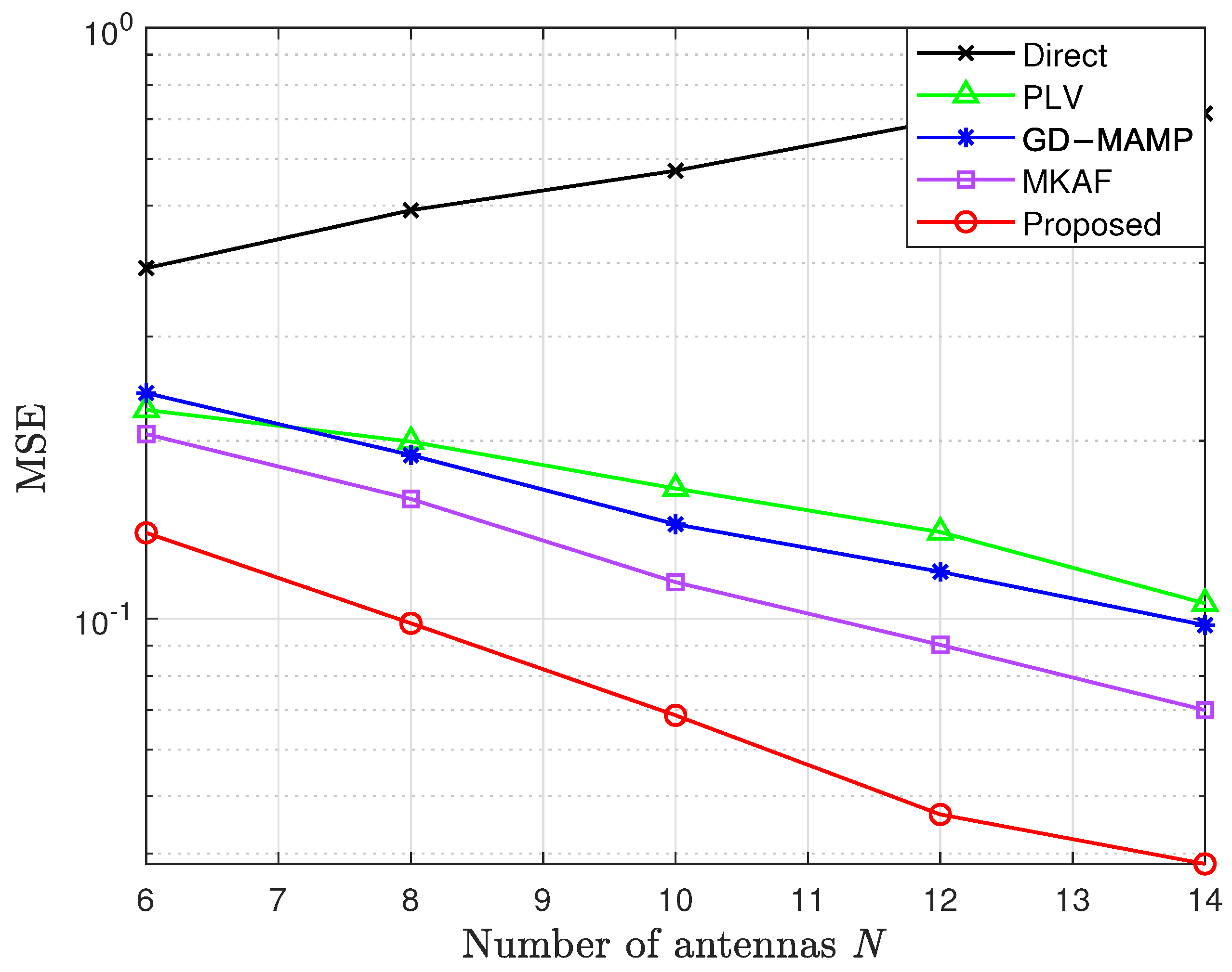
4.1. Simulation Performance Under an Ideal Channel Model

We employ a 2D model following [20,33] to characterize the APS, positing that it is constituted by the superposition of several Gaussian functions: ρ ( θ ) = q = 1 Q α q f q ( θ ) , where f q N ( ϕ q , Δ q 2 ) . ϕ q is uniformly selected from [ π / 3 , π / 3 ] and Δ q is uniformly selected from [ 3 , 8 ] . α q is uniformly selected from [ 0 , 1 ] satisfying q = 1 Q α q = 1 and Q is uniformly drawn from { 1 , 2 , 3 , 4 , 5 } . Then, R u and R d can be obtained by (2) based on the APS.
The ULA wavelength is λ = 3 · 10 8 / f , where the UL frequency is f u = 1.9 GHz and the DL frequency is f d = 2.1 GHz. The antenna spacing d is set to a half of the UL wavelength.
The accuracy of APS estimation is assessed using the MSE e ( ρ , ρ ^ ) : = E [ ρ ρ ^ F 2 / ρ F 2 ] . For DL CCM estimation, the accuracy is evaluated using e ( R d , R ^ d ) : = E [ R d R ^ d F 2 / R d F 2 ] .
We compare the performance of the proposed algorithm with the following algorithms:
  • PLV algorithm in [20]: Based on optimization theory, this algorithm estimates the APS from the UL CCM and achieves the CCM conversion by employing projection methods in an infinite-dimensional Hilbert space.
  • Gradient Descent Memory AMP (GD-MAMP) in [34]: This algorithm is designed to address CS problems by integrating gradient descent with an AMP framework. It efficiently estimates the APS from the UL CCM, thereby deriving an accurate estimate of the DL CCM.
  • MKAF algorithm in [35]: This algorithm models the APS using Gaussian kernels, directly updating the parameters of the kernels based on the UL CCM, and reconstructs the DL CCM according to the estimated APS.
Figure 3, Figure 4, Figure 5 and Figure 6 present the estimation results of APS and DL CCM under four different scenarios: unimodal with smaller angular spread, unimodal with larger angular spread, multi-modal with smaller angular spread, and multi-modal with larger angular spread, respectively. The simulation results demonstrate that the proposed algorithm outperforms the other three benchmark methods, exhibiting robust performance across different APS distributions.
Intuitively, the proposed algorithm improves performance by effectively utilizing the sparsity and structural characteristics of the APS. Specifically, The OAMP module utilizes the sparsity to obtain an initial APS estimation from the UL CCM, whereas the MKAF module refines the APS estimation by leveraging its structural characteristics. These two modules operate iteratively, progressively improving the accuracy of APS estimation and DL CCM estimation. Nevertheless, we notice that both the PLV and GD-MAMP algorithms are based on a discrete grid of a spectrum, which leads to spectral leakage for a practical continuous spectrum. The MKAF algorithm directly estimates the parameters related to the modeling of the APS based on the UL CCM, which is a highly complex problem, resulting in less accurate estimation.
Figure 7 shows the MSE performance of APS estimation under different numbers of antennas N. The results are based on 100 realizations of diverse APS distributions with the angular spread in the range of [ 3 , 8 ] and the number of peaks in the range of [ 1 , 5 ] . It can be observed that the performance of all algorithms improves with an increase in the number of antennas. Moreover, the proposed Turbo-CCC algorithm outperforms the other three algorithms, which is attributed to the fact that the proposed algorithm fully exploits the sparsity and structural characteristics of the APS through its iterative optimization mechanism.
Figure 8 shows the MSE performance of DL CCM reconstruction under different numbers of antennas N. The results are also based on 100 realizations of diverse APS distributions. To highlight the performance of various algorithms, we also included the performance of direct UL-DL CCM conversion. Similar to the observation in Figure 7, the performance of all algorithms improves with an increase in the number of antennas. The performance of the proposed algorithm is generally better than the other three algorithms. This is expected, as the proposed algorithm makes full use of the sparsity and structural characteristics of the APS, resulting in a more accurate estimation of the APS, and consequently, a more accurate reconstruction of the DL CCM.

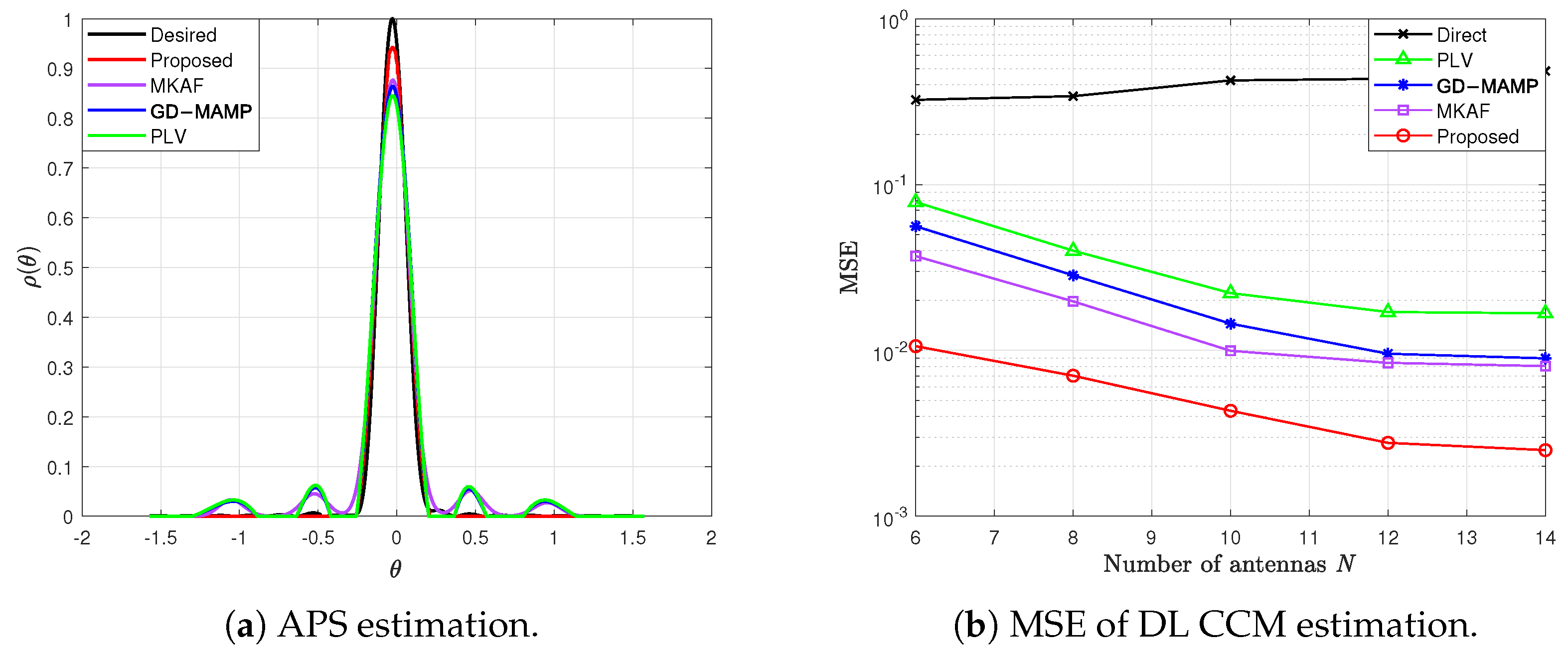
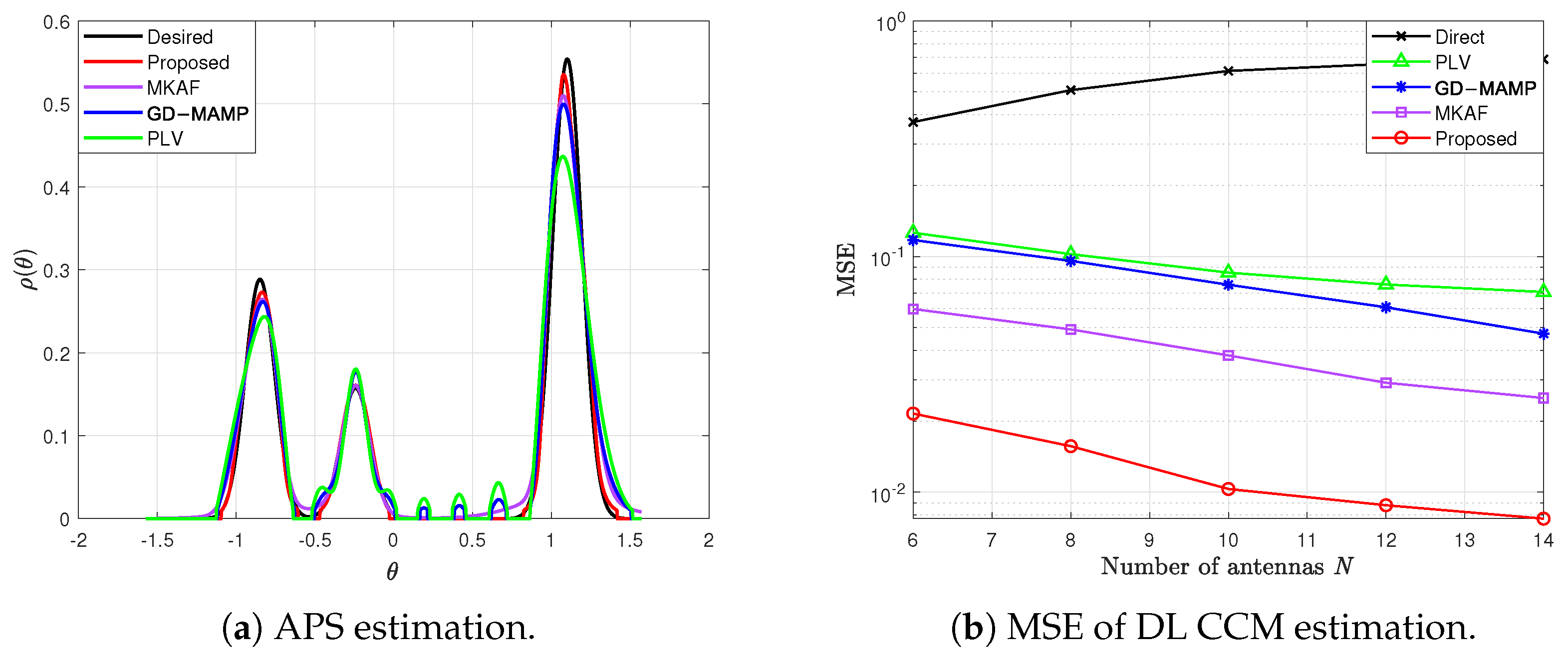
4.2. Simulation Performance Under a CDL Channel Model

In this section, we replace the custom-generated APS with a realistic APS to ensure more robust results. We utilize the MATLAB R2022a CDL channel model, which is designed to simulate real-world communication scenarios by modeling the multipath environment, to generate the realistic APS. We obtain the APS based on the CDL channel data, and then use it in Equation (2) to compute the covariance matrix R u and R d . The channel parameters for the CDL model are defined as follows:
  • Delay Spread = 100 ns: A delay spread of 100 ns is assumed, representing the temporal dispersion of multipath components.
  • DopplerShift = 30 Hz: Doppler shifts are calculated based on the relative velocity between the transmitter and the receiver.
  • AngularSpread = 3°–10°: The angular spread is set to 3°–10° to represent the angular dispersion of multipath components, typical in urban scenarios where reflections from buildings and other obstacles cause multi-pathing.
Figure 9 and Figure 10 present the MSE performance of APS estimation and DL CCM estimation under the CDL channel model, respectively. Similar to the previous simulations, the performance of the proposed algorithm is based on 100 realizations of diverse APS distributions. The results demonstrate that the proposed algorithm achieves lower MSE values compared to the baseline methods in both APS estimation and DL CCM estimation. This improvement is attributed to the algorithm’s ability to take full advantage of the sparsity and structural characteristics of the APS. The results underscore the robustness of the proposed algorithm in handling realistic APS scenarios, further validating its superiority in practical communication systems.

5. Discussion

The results of this study demonstrate the effectiveness of the proposed Turbo-CCC algorithm in addressing the challenging problem of DL CCM estimation in massive MIMO FDD systems. By integrating the OAMP algorithm with the MKAF algorithm under a Bayesian framework, the proposed algorithm achieves improvements in accuracy and robustness compared to existing approaches. The key innovation lies in the extraction of APS information based on the sparsity and structural characteristics of the APS, which is utilized to enhance the estimation process. The algorithm’s versatility is further highlighted by its ability to adapt to a wide range of APS distributions, making it suitable for diverse practical scenarios. The proposed algorithm can enhance the CSI acquisition for MIMO systems, which is crucial for optimizing the performance and capacity of MIMO systems. In future research, we could conduct a convergence analysis based on a recent non-asymptotic work [36], which sheds light on a possible fully rigorous proof for the convergence behavior. Moreover, we can also explore combining the algorithm with machine learning techniques, adapting it to dynamic environments, or further optimizing computational efficiency for next-generation wireless networks.

Author Contributions

Methodology, Z.Y., S.L. and C.X.; software, Z.Y.; resources, C.X. and Z.Y.; writing—original draft preparation, Z.Y.; writing—review and editing, Z.Y., C.X. and S.L. All authors have read and agreed to the published version of the manuscript.

Funding

This work was supported by the National Natural Science Foundation of China under Grant 62271154.

Data Availability Statement

The data presented in this study are available upon reasonable request from the corresponding author.

Conflicts of Interest

The authors declare no conflicts of interest.

References

  1. Björnson, E.; Hoydis, J.; Sanguinetti, L. Massive MIMO networks: Spectral, energy, and hardware efficiency. Found. Trends® Signal Process. 2017, 11, 154–655. [Google Scholar] [CrossRef]
  2. Marzetta, T.L. Noncooperative cellular wireless with unlimited numbers of base station antennas. IEEE Trans. Wirel. Commun. 2010, 9, 3590–3600. [Google Scholar] [CrossRef]
  3. Rusek, F.; Persson, D.; Lau, B.K.; Larsson, E.G.; Marzetta, T.L.; Edfors, O.; Tufvesson, F. Scaling up MIMO: Opportunities and challenges with very large arrays. IEEE Signal Process. Mag. 2012, 30, 40–60. [Google Scholar] [CrossRef]
  4. Kocian, A.; Badiu, M.A.; Fleury, B.H.; Martelli, F.; Santi, P. A unified message-passing algorithm for MIMO-SDMA in software-defined radio. EURASIP J. Wirel. Commun. Netw. 2017, 2017, 4. [Google Scholar] [CrossRef]
  5. He, H.; Yu, X.; Zhang, J.; Song, S.; Letaief, K.B. Message passing meets graph neural networks: A new paradigm for massive MIMO systems. IEEE Trans. Wirel. Commun. 2023, 23, 4709–4723. [Google Scholar] [CrossRef]
  6. Bellili, F.; Sohrabi, F.; Yu, W. Generalized approximate message passing for massive MIMO mmWave channel estimation with Laplacian prior. IEEE Trans. Commun. 2019, 67, 3205–3219. [Google Scholar] [CrossRef]
  7. Wang, H.; Xu, L.; Yan, Z.; Gulliver, T.A. Low-complexity MIMO-FBMC sparse channel parameter estimation for industrial big data communications. IEEE Trans. Ind. Inform. 2020, 17, 3422–3430. [Google Scholar] [CrossRef]
  8. Peng, Q.; Huang, Y.; Zhou, W. Graph Neural Network-Based Low-Complexity Channel Estimation for Massive MU-MIMO Systems. In Proceedings of the 2024 9th International Conference on Computer and Communication Systems (ICCCS), Xi’an, China, 19–22 April 2024; pp. 623–628. [Google Scholar]
  9. Ma, Y.; He, H.; Song, S.; Zhang, J.; Letaief, K.B. Low-complexity CSI feedback for FDD massive MIMO systems via learning to optimize. IEEE Trans. Wirel. Commun. 2025. [Google Scholar] [CrossRef]
  10. Xie, H.; Gao, F.; Jin, S.; Fang, J.; Liang, Y.C. Channel estimation for TDD/FDD massive MIMO systems with channel covariance computing. IEEE Trans. Wirel. Commun. 2018, 17, 4206–4218. [Google Scholar] [CrossRef]
  11. De Figueiredo, F.A.; Cardoso, F.A.; Moerman, I.; Fraidenraich, G. Channel estimation for massive MIMO TDD systems assuming pilot contamination and frequency selective fading. IEEE Access 2017, 5, 17733–17741. [Google Scholar] [CrossRef]
  12. Chan, P.W.; Lo, E.S.; Wang, R.R.; Au, E.K.; Lau, V.K.; Cheng, R.S.; Mow, W.H.; Murch, R.D.; Letaief, K.B. The evolution path of 4G networks: FDD or TDD? IEEE Commun. Mag. 2006, 44, 42–50. [Google Scholar] [CrossRef]
  13. Jordan, M.; Dimofte, A.; Gong, X.; Ascheid, G. Conversion from uplink to downlink spatio-temporal correlation with cubic splines. In Proceedings of the VTC Spring 2009-IEEE 69th Vehicular Technology Conference, Barcelona, Spain, 26–29 April 2009; pp. 1–5. [Google Scholar]
  14. Haghighatshoar, S.; Khalilsarai, M.B.; Caire, G. Multi-band covariance interpolation with applications in massive MIMO. In Proceedings of the 2018 IEEE International Symposium on Information Theory (ISIT), Vail, CO, USA, 17–22 June 2018; pp. 386–390. [Google Scholar]
  15. Decurninge, A.; Guillaud, M.; Slock, D. Riemannian coding for covariance interpolation in massive MIMO frequency division duplex systems. In Proceedings of the 2016 IEEE Sensor Array and Multichannel Signal Processing Workshop (SAM), Rio de Janeiro, Brazil, 10–13 July 2016; pp. 1–5. [Google Scholar]
  16. Zou, L.; Pan, Z.; Jiang, H.; Liu, N.; You, X. Deep learning based downlink channel covariance estimation for FDD massive MIMO systems. IEEE Commun. Lett. 2021, 25, 2275–2279. [Google Scholar]
  17. Hugl, K.; Kalliola, K.; Laurila, J. Spatial reciprocity of uplink and downlink radio channels in FDD systems. In Proceedings of the COST 273 Meeting, Espoo, Finland, 30–31 May 2002; Volume 273, p. 066. [Google Scholar]
  18. Zhong, Z.; Fan, L.; Ge, S. FDD massive MIMO uplink and downlink channel reciprocity properties: Full or partial reciprocity? In Proceedings of the GLOBECOM 2020-2020 IEEE Global Communications Conference, Taipei, Taiwan, 7–11 December 2020; pp. 1–5. [Google Scholar]
  19. Park, S.; Heath, R.W. Spatial channel covariance estimation for the hybrid MIMO architecture: A compressive sensing-based approach. IEEE Trans. Wirel. Commun. 2018, 17, 8047–8062. [Google Scholar] [CrossRef]
  20. Miretti, L.; Cavalcante, R.L.G.; Stańczak, S. Channel covariance conversion and modelling using infinite dimensional Hilbert spaces. IEEE Trans. Signal Process. 2021, 69, 3145–3159. [Google Scholar] [CrossRef]
  21. Vesperinas, M.N. Scattering and Diffraction in Physical Optics; World Scientific Publishing Company: Singapore, 2006. [Google Scholar]
  22. Burr, A. The multipath problem: An overview. In Proceedings of the IEE Colloquium on Multipath Countermeasures, London, UK, 23–23 May 1996; p. 1. [Google Scholar]
  23. Ninomiya, E.; Yukawa, M.; Cavalcante, R.L.; Miretti, L. Estimation of angular power spectrum using multikernel adaptive filtering. In Proceedings of the 2022 Asia-Pacific Signal and Information Processing Association Annual Summit and Conference (APSIPA ASC), Chiang Mai, Thailand, 7–10 November 2022; pp. 1996–2000. [Google Scholar]
  24. Elshirkasi, A.M.; Al-Hadi, A.A.; Mansor, M.F.; Khan, R.; Soh, P.J. Envelope correlation coefficient of a two-port MIMO terminal antenna under uniform and Gaussian angular power spectrum with user’s hand effect. Prog. Electromagn. Res. C 2019, 92, 123–136. [Google Scholar]
  25. Tse, D.; Viswanath, P. Fundamentals of Wireless Communication; Cambridge University Press: Cambridge, UK, 2005. [Google Scholar]
  26. Björnson, E.; Larsson, E.G.; Marzetta, T.L. Massive MIMO: Ten myths and one critical question. IEEE Commun. Mag. 2016, 54, 114–123. [Google Scholar]
  27. Takizawa, M.A.; Yukawa, M. Online learning with self-tuned Gaussian kernels: Good kernel-initialization by multiscale screening. In Proceedings of the ICASSP 2019-2019 IEEE International Conference on Acoustics, Speech and Signal Processing (ICASSP), Brighton, UK, 12–17 May 2019; pp. 4863–4867. [Google Scholar]
  28. Ma, J.; Ping, L. Orthogonal AMP. IEEE Access 2017, 5, 2020–2033. [Google Scholar]
  29. Yamamoto, T.; Yamagishi, M.; Yamada, I. Adaptive proximal forward-backward splitting for sparse system identification under impulsive noise. In Proceedings of the 2012 Proceedings of the 20th European Signal Processing Conference (EUSIPCO), Bucharest, Romania, 27–31 August 2012; pp. 2620–2624. [Google Scholar]
  30. Beck, A.; Teboulle, M. Mirror descent and nonlinear projected subgradient methods for convex optimization. Oper. Res. Lett. 2003, 31, 167–175. [Google Scholar] [CrossRef]
  31. Amari, S.i. Backpropagation and stochastic gradient descent method. Neurocomputing 1993, 5, 185–196. [Google Scholar] [CrossRef]
  32. Mimura, K.; Takeuchi, J. Dynamics of damped approximate message passing algorithms. In Proceedings of the 2019 IEEE Information Theory Workshop (ITW), Visby, Sweden, 25–28 August 2019; pp. 1–5. [Google Scholar]
  33. Goldsmith, A. Wireless Communications; Cambridge University Press: Cambridge, UK, 2005. [Google Scholar]
  34. Huang, S.; Liu, L.; Kurkoski, B.M. Overflow-avoiding memory AMP. In Proceedings of the 2024 IEEE International Symposium on Information Theory (ISIT), Athens, Greece, 7–12 July 2024; pp. 3516–3521. [Google Scholar]
  35. Kaneko, N.; Yukawa, M.; Cavalcante, R.L.; Miretti, L. Robust estimation of angular power spectrum in massive MIMO under covariance estimation errors: Learning centers and scales of Gaussians. In Proceedings of the 2024 IEEE 25th International Workshop on Signal Processing Advances in Wireless Communications (SPAWC), Lucca, Italy, 10–13 September 2024; pp. 576–580. [Google Scholar]
  36. Cademartori, C.; Rush, C. A non-asymptotic analysis of generalized vector approximate message passing algorithms with rotationally invariant designs. IEEE Trans. Inf. Theory 2024, 70, 5811–5856. [Google Scholar] [CrossRef]
Figure 1. APS approximation with Gaussian functions.
Electronics 14 01490 g001
Figure 2. The diagram of the Turbo-CCC algorithm.
Electronics 14 01490 g002
Figure 3. Performance of APS estimation and DL CCM estimation under unimodal distribution with smaller angular spread.
Electronics 14 01490 g003
Figure 4. Performance of APS estimation and DL CCM estimation under unimodal distribution with larger angular spread.
Electronics 14 01490 g004
Figure 5. Performance of APS estimation and DL CCM estimation under multi-modal distribution with smaller angular spread.
Electronics 14 01490 g005
Figure 6. Performance of APS estimation and DL CCM estimation under multi-modal distribution with larger angular spread.
Electronics 14 01490 g006
Figure 7. MSE performance of APS estimation with different numbers of antennas N under ideal channel model.
Electronics 14 01490 g007
Figure 8. MSE performance of DL CCM estimation with different numbers of antennas N under ideal channel model.
Electronics 14 01490 g008
Figure 9. MSE performance of APS estimation with different numbers of antennas N under CDL channel model.
Electronics 14 01490 g009
Figure 10. MSE performance of DL CCM estimation with different numbers of antennas N under CDL channel model.
Electronics 14 01490 g010
Disclaimer/Publisher’s Note: The statements, opinions and data contained in all publications are solely those of the individual author(s) and contributor(s) and not of MDPI and/or the editor(s). MDPI and/or the editor(s) disclaim responsibility for any injury to people or property resulting from any ideas, methods, instructions or products referred to in the content.

