Data Throughput-Oriented Site Selection: Integrated Downlink Scheduling with Elastic Laser Communication Terminal Deployment

Abstract

Space-to-ground laser communication (SGLC) offers a paradigm-shifting solution to overcome the bandwidth constraints of radio frequency systems by leveraging laser beams for ultra-high data throughput, although its link availability probability is significantly affected by atmospheric conditions such as cloud cover. Existing ground station (GS) placement methods decouple site selection from downlink scheduling, failing to effectively quantify the data throughput of candidate sites. This study proposes a data throughput-driven joint optimization framework that integrates downlink scheduling into the site selection model for the first time. Additionally, the site selection model also incorporates equipment cost constraints and service capacity limitations by introducing an integer variable Q to characterize the deployment scale of laser communication terminals (LCTs) at each GS. Through auxiliary variable linearization techniques, the site selection problem is transformed into a tractable integer linear programming (ILP) formulation. A branch-and-bound algorithm is proposed to achieve global optimal solution search. Numerical results demonstrate that the proposed approach improves data throughput compared to the existing method.

1. Introduction

Space-to-ground laser communication (SGLC) presents a paradigm-shifting alternative to bandwidth-constrained radio frequency (RF) systems by leveraging laser beams to achieve unprecedented data throughput (exceeding conventional RF by orders of magnitude) while eliminating spectral licensing requirements [1,2,3,4]. Such advantages have positioned SGLC as an enabling technology for space applications, particularly in geostationary satellite-based weather forecasting, climate modeling, emergency response coordination, and deep-space exploration missions where real-time transfer of massive datasets (including hyperspectral imagery and multidimensional sensing data) is mission-critical [5,6,7,8].

However, SGLC is notably impaired by atmospheric conditions, particularly cloud cover [9]. Cloud presence along the satellite-to-ground laser link path causes signal interruption through strong absorption and scattering effects [10,11,12]. Link availability probabilityis defined as a continuous value in the range $[0,1]$, representing the fraction of a time slot during which the laser link remains successfully connected. For example, during a 10-s interval with 2 s of cloud-induced disconnection, the link availability probability calculates to $(10-2)/10=0.8$. This metric quantitatively measures the temporal connectivity reliability between satellites and GSs, where persistent cloud coverage directly determines the laser link’s operational duration.

The spatiotemporal variability of cloud blockage induces significant fluctuations in the link availability probability of space-to-ground laser links across temporal and spatial domains. This necessitates the intelligent scheduling of satellite downlink operations to circumvent adverse atmospheric impacts—a process termed downlink scheduling [13,14,15]. The core objective is to maximize the data throughput, defined as the total downloaded data to the GSs within a scheduling horizon, by strategically selecting GSs for each satellite based on parameters such as link availability probability. The scheduling horizon is partitioned into equal-duration intervals, with satellite-GS pairing decisions updated at the end of each interval (satellite switch to another GS). The performance ceiling of downlink scheduling is ultimately dictated by the geographic configuration of GSs [15], making site selection for GSs (or placement for GSs) a pivotal determinant of overall network capability. This is because the spatial distribution of stations directly governs the link availability probability of a satellite–GS pair, which influences the downloaded data within a scheduling horizon.

The site selection optimization problem for SGLC systems can be defined as follows: selecting an optimal station combination from a given candidate site set under constraints such as system availability and deployment cost to achieve the global optimization of system objectives (e.g., minimizing deployment costs). As illustrated in Figure 1, the candidate ground station set is $\{GroundStation1,GroundStation2,GroundStation3,GroundStation4\}$.

Figure 1 demonstrates the availability-constrained ground station site selection strategy, taking an SGLC system with one GEO satellite and four candidate ground stations as an example under a scheduling period of one time slot. The red and green bidirectional solid lines represent different site selection strategies. Site selection strategy 1 (red bidirectional solid lines) chooses GS1 and GS4 as construction sites. However, in the current time slot, both space–ground laser links are interrupted, failing to meet the availability constraint (i.e., requiring at least one unblocked space–ground laser link). In contrast, site selection strategy 2 (green bidirectional solid lines) selects GS2 and GS3 as construction sites, ensuring at least one operational space–ground laser link exists, thereby representing a feasible site selection solution.

Existing studies [16,17,18,19,20,21,22] have investigated the site selection problem in satellite communication systems. Analyses of GS minimization strategies were conducted for distinct orbital architectures in [16] (medium Earth orbit systems) and [17] (geostationary systems), with both methodologies employing computationally efficient heuristic algorithms that systematically account for spatial cloud coverage correlations and monthly meteorological variability patterns. The authors in [18] develop an optical GS selection method considering both site-specific availability and inter-site correlations. The authors of [19] propose a two-part optimization approach for satellite networks: GS positioning and fiber-cost-aware backbone network design. Recent advancements in GS selection methodologies include a gradient-projection algorithm for availability-maximized FSO (free space optical) network configurations in [20], demonstrating polynomial-time computational efficiency in selecting predefined GS quantities. Concurrently, Ref. [21] introduced a site selection framework that achieves deterministic global optimality in minimum-cardinality GS selection while satisfying time-varying availability constraints, with computational complexity scaling linearly with network density. The authors of [22] addressed cost-optimal GS selection in hybrid RF/optical satellite networks under system availability constraints, proposing a globally optimal dynamic programming algorithm and a polynomial-time approximation scheme with bounded optimality gaps.

Current availability-driven GS selection paradigms [16,17,18,19,20,21,22] fail to satisfy the escalating data throughput requirements of modern space-to-ground data delivery systems, as their design frameworks specifically target MEO/GEO scenarios with system availability-centric optimization metrics (ensuring at least one viable link connectivity). Furthermore, such site selection models decouple GS placement from data throughput analysis, lacking built-in mechanisms to directly evaluate end-to-end system data throughput. This paper establishes a data throughput-centric paradigm for site selection problem, and the main contributions are as follows:

• We propose a tightly-coupled optimization model that holistically integrates geographic site selection with downlink scheduling, enabling quantitative evaluation of end-to-end data throughput performance across different candidate GS configurations.
• The proposed model incorporates an integer decision variable Q to characterize the LCT deployment scale at each GS, explicitly embedding equipment cost constraints and service capacity limitations for enhanced operational fidelity.
• The model is subsequently transformed into a tractable integer linear programming (ILP) [23,24,25] formulation through the introduction of auxiliary variables.
• A branch-and-bound algorithm is developed to solve the ILP problem, with numerical simulations demonstrating superior data throughput over existing solutions under equivalent installation cost constraints.

The paper is structured as follows: Section 2 first presents the system model, followed by a formulation of the site selection problem and its linearization. A branch-and-bound algorithm is developed to solve the ILP problem in Section 3. Simulation results are given in Section 4. Conclusions and future research perspectives are presented in Section 5.

2. System Model and Problem Formulation

Consider a space–ground laser communication system comprising S low Earth orbit (LEO) satellites, one geostationary (GEO) satellite, and G candidate GSs. Specifically, let $\mathcal{G}=\{1,2,\dots ,G\}$ denote the set of candidate GSs, $\mathcal{S}=\{1,2,\dots ,S\}$ the LEO satellite constellation, and $\mathcal{T}=\{1,2,\dots ,T\}$ the time period set (e.g., measured in days or months). All candidate GSs remain continuously visible to the GEO satellite. The term $p_{t,s,g}^{avb}(t\in \mathcal{T},s\in \mathcal{S},g\in \mathcal{G})$ represents the link availability probability between the s-th LEO satellite and g-th GS during period t, while $p_{t,g}^{avb}(t\in \mathcal{T},g\in \mathcal{G})$ denotes the corresponding probability for GEO-GS links. These probabilities are statistically derived from historical data quantifying the percentage of time maintaining bidirectional laser communication, primarily affected by cloud blockage. The system model operates under the following assumptions:

• Each LEO satellite carries a single LCT for space–ground links due to size, weight, and power constraints;
• The GEO satellite can be equipped with up to G LCTs, enabling potential connectivity with all candidate GSs;
• Availability probabilities $p_{t,g}^{avb}$ and $p_{t,s,g}^{avb}$ are considered statistically independent when GSs are sufficiently spaced, neglecting spatial weather correlations;
• To reduce the computational complexity of the problem, we assume that the link availability probabilities $p_{t,g}^{avb}$ (for GEO-to-GS links) and $p_{t,s,g}^{avb}$ (for LEO-to-GS links) remain fixed within each time slot;
• LEO satellites maintain fixed laser links with single GSs per time period, permitting dynamic link switching between periods.

The data throughput ($Data$) of the SGLC system is formulated as follows:

$$\begin{array}{c}Data=\sum _{t=1}^T\sum _{s=1}^S\sum _{g=1}^G(\mathsf{\Delta }{t}_{t,s,g}·{\varphi }_{t,s,g}·p_{t,s,g}^{avb}·x_{t,s,g})·z_g+\\ \sum _{t=1}^T\sum _{g=1}^G(\mathsf{\Delta }{t}_{t,g}·{\varphi }_{t,g}·p_{t,g}^{avb}·y_{t,g})·z_g,\end{array}$$

(1)

where

• T, S, and G denote the total number of time periods, LEO satellites, and candidate GSs, respectively;
• $\mathsf{\Delta }{t}_{t,s,g}$ quantifies the visible time window (measured in seconds) between the s-th LEO satellite and the g-th GS during period t, with $\mathsf{\Delta }{t}_{t,g}$ representing the GEO-GS visibility duration;
• ${\varphi }_{t,s,g}$ and ${\varphi }_{t,g}$ indicate the data transfer rates for LEO-GS and GEO-GS links, respectively;
• Binary variables $x_{t,s,g}\in \{0,1\}$ and $y_{t,g}\in \{0,1\}$ activate LEO-GS and GEO-GS links when equal to 1 (downlink scheduling variables);
• Site selection variable $z_g\in \{0,1\}$ determines the GS deployment at location g, and $z_g=1$ indicates the g-th candidate GS is selected (or, equivalently, a GS is installed at the g-th location).

As shown in Equation (2), the data throughput calculation requires both GS deployment ($z_g=1$) and laser link activation ($x_{t,s,g}=1$ or $y_{t,g}=1$).

The GS deployment cost comprises base and incremental capacity costs:

$$c_g\left(Q\right)=c_g^{base}+C_{LCT}·(Q-1),\forall g\in \mathcal{G},Q\ge 1,$$

(2)

where $c_g^{base}$ denotes the base cost for the GS with one LCT, and $C_{LCT}$ represents the marginal cost per additional LCT. This model exhibits linear cost scaling: $Q=1$ incurs only $c_g^{base}$, while $Q>1$ adds $C_{LCT}·(Q-1)$. Physically, each LCT enables an additional concurrent laser link bounded by $Q\le L_{up}$ (maximum LCT installations per GS).

2.1. Problem Formulation

The core objective of the site selection optimization model is to maximize the data throughput of the space–ground laser communication system under total deployment cost constraints by jointly optimizing four decision variables: GS deployment $\left\{z_g\right\}$, LEO downlink scheduling $\left\{x_{t,s,g}\right\}$, GEO downlink scheduling $\left\{y_{t,g}\right\}$, and LCT configuration quantity $\left\{Q\right\}$. Compared to existing site selection models, our innovations include (1) integrating downlink scheduling decisions ($\left\{x_{t,s,g}\right\}$ and $\left\{y_{t,g}\right\}$) into the site selection model to enable dynamic throughput capacity evaluation and (2) constructing a compound site selection model with integer variable Q representing the LCT deployment scale, incorporating equipment costs and service capacity constraints. Notably, “Elastic” refers to the approach where GSs are not pre-equipped with a fixed number of LCTs. Instead, the quantity of LCTs at each ground station is treated as a decision variable within the site selection optimization model.

$$\begin{array}{c}\underset{\left\{x_{t,s,g}\right\},\left\{y_{t,g}\right\},\left\{z_g\right\},\left\{Q\right\}}{\max }\sum _{t=1}^T\sum _{s=1}^S\sum _{g=1}^G({\alpha }_{t,s,g}·x_{t,s,g})·z_g+\sum _{t=1}^T\sum _{g=1}^G({\beta }_{t,g}·y_{t,g})·z_g\end{array}$$

(3)

$$\begin{array}{c}\mathrm{s}.\mathrm{t}. \sum _{s=1}^S{x}_{t,s,g}+y_{t,g}\le Q·z_g,\forall t\in \mathcal{T},g\in \mathcal{G}\end{array}$$

(4)

$$\begin{array}{c}\sum _{g=1}^G{x}_{t,s,g}\le 1,\forall t\in \mathcal{T},s\in \mathcal{S}\end{array}$$

(5)

$$\begin{array}{c}\sum _{g=1}^G{y}_{t,g}\le G,\forall t\in \mathcal{T}\end{array}$$

(6)

$$\begin{array}{c}{x}_{t,s,g}\le z_g,\forall t\in \mathcal{T},s\in \mathcal{S},g\in \mathcal{G}\end{array}$$

(7)

$$\begin{array}{c}{y}_{t,g}\le z_g,\forall t\in \mathcal{T},g\in \mathcal{G}\end{array}$$

(8)

$$\begin{array}{c}\sum _{g=1}^G(c_g^{base}+C_{LCT}·(Q-1))·z_g\le C_{up}\end{array}$$

(9)

$$\begin{array}{c}1\le Q\le L_{up},\forall g\in \mathcal{G}\end{array}$$

(10)

$$\begin{array}{c}{x}_{t,s,g}\in \{0,1\},\forall t\in \mathcal{T},s\in \mathcal{S},g\in \mathcal{G}\end{array}$$

(11)

$$\begin{array}{c}{y}_{t,g}\in \{0,1\},\forall t\in \mathcal{T},g\in \mathcal{G}\end{array}$$

(12)

$$\begin{array}{c}{z}_g\in \{0,1\},\forall g\in \mathcal{G}\end{array}$$

(13)

$$\begin{array}{c}Q\in {\mathbb{Z}}^{+},\end{array}$$

(14)

where ${\alpha }_{t,s,g}=\mathsf{\Delta }{t}_{t,s,g}·{\varphi }_{t,s,g}·p_{t,s,g}^{avb}$, and ${\beta }_{t,g}=\mathsf{\Delta }{t}_{t,g}·{\varphi }_{t,g}·p_{t,g}^{avb}$. The objective function (3) aims to maximize data throughput. Key constraints include the following:

• (4) limits concurrent laser links per GS to Q;
• (5) and (6) restrict LEO satellites to single connections and GEO satellites to maximum G connections;
• (7) and (8) enforce link activation only at deployed GSs ($z_g=1$);
• (9) has a total deployment cost cap $C_{up}$;
• (10) has LCT installation bounds $[1,L_{up}]$;
• (11)–(13) has binary variable definitions;
• (14) contains an integer constraint for LCT quantities.

The proposed model exhibits intrinsic nonlinear combinatorial characteristics originating from two fundamental sources: (1) multiplicative interactions between scheduling binary variables and deployment binary variables (e.g., $x_{t,s,g}·z_g$, $y_{t,g}·z_g$) and (2) integer–binary variable couplings governing the capacity limitation of each GS (e.g., $Q·z_g$). These nonlinear terms necessitate linearization to enable tractable computation.

It is noted that the proposed site selection model possesses extensibility to other constellations, notably those employing laser/microwave hybrid links. This adaptability stems from the fact that a satellite equipped with both LCT and RF transceivers can be functionally equivalent to two distinct satellites—one carrying LCT payloads and the other RF systems. Furthermore, the model’s differentiation across constellations manifests exclusively in parametric variations of input parameters such as link availability probabilities and data transmission rates.

2.2. Linearization of the Problem

The linearization process specifically addresses bilinear product terms through auxiliary variables. For the binary–binary products, we introduce auxiliary variables:

$$\begin{array}{c}{u}_{t,s,g}=x_{t,s,g}·z_g,v_{t,g}=y_{t,g}·z_g\end{array}$$

(15)

$$\begin{array}{c}{u}_{t,s,g}\le x_{t,s,g},\forall t\in \mathcal{T},s\in \mathcal{S},g\in \mathcal{G}\end{array}$$

(16)

$$\begin{array}{c}{u}_{t,s,g}\le z_g,\forall t\in \mathcal{T},s\in \mathcal{S},g\in \mathcal{G}\end{array}$$

(17)

$$\begin{array}{c}{u}_{t,s,g}\ge x_{t,s,g}+z_g-1,\forall t\in \mathcal{T},s\in \mathcal{S},g\in \mathcal{G}\end{array}$$

(18)

$$\begin{array}{c}{v}_{t,g}\le y_{t,g},\forall t\in \mathcal{T},g\in \mathcal{G}\end{array}$$

(19)

$$\begin{array}{c}{v}_{t,g}\le z_g,\forall t\in \mathcal{T},g\in \mathcal{G}\end{array}$$

(20)

$$\begin{array}{c}{v}_{t,g}\ge y_{t,g}+z_g-1,\forall t\in \mathcal{T},g\in \mathcal{G}\end{array}$$

(21)

$$\begin{array}{c}{x}_{t,s,g},y_{t,g},z_g,u_{t,s,g},v_{t,g}\in \{0,1\}.\end{array}$$

(22)

Constraint Validation: Consider $v_{t,g}=y_{t,g}·z_g$. The product equals 1 iff $y_{t,g}=z_g=1$, enforced by $v_{t,g}\le \min (y_{t,g},z_g)$ and $v_{t,g}\ge y_{t,g}+z_g-1$. When either variable is 0, $v_{t,g}$ is forced to 0.

For integer–binary products $w_g=Q·z_g$, we introduce auxiliary variable $w_g$ with constraints:

$$\begin{array}{c}{w}_g\le L_{\mathrm{up}}·z_g(\mathrm{forces} w_g=0 \mathrm{when} z_g=0)\end{array}$$

(23)

$$\begin{array}{c}{w}_g\le Q(\mathrm{upper} \mathrm{bounds} \mathrm{by} \mathrm{LCT} \mathrm{quantity})\end{array}$$

(24)

$$\begin{array}{c}{w}_g\ge Q-L_{\mathrm{up}}(1-z_g)(\mathrm{forces} w_g=Q \mathrm{when} z_g=1)\end{array}$$

(25)

$$\begin{array}{c}{w}_g\ge 0\left(\mathrm{non}\text{-}\mathrm{negativity}\right)\end{array}$$

(26)

$$\begin{array}{c}Q\in \{1,\dots ,L_{\mathrm{up}}\},z_g\in \{0,1\}.\end{array}$$

(27)

The linearized site selection model becomes

$$\begin{array}{c}\underset{\begin{array}{c}\{x,y,z,Q,\\ u,v,w\}\end{array}}{\max }\sum _{t,s,g}{\alpha }_{t,s,g}{u}_{t,s,g}+\sum _{t,g}{\beta }_{t,g}{v}_{t,g}\end{array}$$

(28)

$$\begin{array}{c}\mathrm{such} \mathrm{that} \sum _s{x}_{t,s,g}+y_{t,g}\le w_g,\forall t,g\end{array}$$

(29)

$$\begin{array}{c}\sum _g{x}_{t,s,g}\le 1,\forall t,s\end{array}$$

(30)

$$\begin{array}{c}\sum _g{y}_{t,g}\le G,\forall t\end{array}$$

(31)

$$\begin{array}{c}{x}_{t,s,g}\le z_g,\forall t,s,g\end{array}$$

(32)

$$\begin{array}{c}{y}_{t,g}\le z_g,\forall t,g\end{array}$$

(33)

$$\begin{array}{c}\sum _g[(c_g^{base}-C_{LCT})z_g+C_{LCT}{w}_g]\le C_{up}\end{array}$$

(34)

$$\begin{array}{c}{w}_g\le L_{up}{z}_g,\forall g\end{array}$$

(35)

$$\begin{array}{c}{w}_g\le Q,\forall g\end{array}$$

(36)

$$\begin{array}{c}{w}_g\ge Q-L_{up}(1-z_g),\forall g\end{array}$$

(37)

$$\begin{array}{c}⋮(\mathrm{all} \mathrm{previous} u/v \mathrm{constraints})\end{array}$$

(38)

$$\begin{array}{c}x,y,z,u,v\in \{0,1\},Q,w_g\in {\mathbb{Z}}^{+},w_g\ge 0.\end{array}$$

(39)

This linearized formulation preserves the original NLIP problem’s semantics while enabling efficient solving through integer linear programming techniques.

3. Branch-and-Bound Algorithm

The site selection problem (28)–(39) constitutes an ILP problem, where all decision variables are integers, and both the objective function and constraints exhibit linearity. Traditional exhaustive methods become computationally prohibitive for practical-scale ILP problems due to their combinatorial explosion property (the solution space grows exponentially with the variable count). Consequently, we developed a branch-and-bound algorithm to address this challenge through synergistic solution space decomposition and bound-based pruning, guaranteeing global optimality without full enumeration. Key algorithmic phases include relaxation problem initialization with bound computation, branching operations, and pruning strategies.

To enhance the model clarity, we reformulate problem (28)–(39) into compact vector notation:

$$\begin{array}{c}\underset{\mathbf{x}}{\min }{\mathbf{c}}^{\top }\mathbf{x}\end{array}$$

(40)

$$\begin{array}{c}\mathbf{A}\mathbf{x}\le \mathbf{b}\end{array}$$

(41)

$$\begin{array}{c}\mathbf{x}\in {\mathbb{Z}}_{\ge 0}^d.\end{array}$$

(42)

Symbol definitions:

• $\mathbf{x}\in {\mathbb{Z}}_{\ge 0}^d$: integer decision vector (dim: $d\times 1$) containing

  −

  Site selection $z_g\in \{0,1\}$ ($G\times 1$)

  −

  Scheduling variables $x_{t,s,g}\in \{0,1\}$ ($T\times S\times G$)

  −

  Scheduling variables $y_{t,g}\in \{0,1\}$ ($T\times G$)

  −

  Auxiliary variables $u_{t,s,g},v_{t,g}\in \{0,1\}$ ($T\times S\times G+T\times G$)

  −

  Auxiliary variables $w_g\in {\mathbb{Z}}^{+}$ ($G\times 1$)

  −

  LCT variable $Q\in {\mathbb{Z}}^{+}$ ($1\times 1$).

• $\mathbf{c}\in {\mathbb{R}}^d$: objective coefficient vector (dim: $d\times 1$)
• $\mathbf{A}\in {\mathbb{R}}^{m\times d}$: constraint matrix (dim: $m\times d$)
• $\mathbf{b}\in {\mathbb{R}}^m$: right-hand-side vector (dim: $m\times 1$).

Dimension calculations:

• Variable dimension:

  $$d=\underset{\mathrm{Sites}}{\underbrace{G}}+\underset{\mathrm{Scheduling}\&\mathrm{Auxiliary}}{\underbrace{2TSG}}+\underset{\mathrm{Scheduling}\&\mathrm{Auxiliary}}{\underbrace{2TG}}+\underset{\mathrm{Auxiliary}\&\mathrm{LCT}}{\underbrace{G+1}}.$$
• Constraint dimension:

  $$m=\underset{\mathrm{Problem} \left(28\right)–\left(39\right) \mathrm{Constraints}}{\underbrace{4TSG+5TG+TS+4G+T+2}}.$$

We relax the integer constraints to obtain the linear programming (LP) relaxation:

$$\begin{array}{c}\underset{\mathbf{x}}{\min }{\mathbf{c}}^{\top }\mathbf{x}\end{array}$$

(43)

$$\begin{array}{c}\mathbf{A}\mathbf{x}\le \mathbf{b}.\end{array}$$

(44)

The LP relaxation’s optimal objective value $Z_{\mathrm{LP}}$ (e.g., $Z_{\mathrm{LP}}=356$) provides a theoretical upper bound for the original ILP. The branch-and-bound algorithm employs three core mechanisms: (1) optimality pruning via bound comparison; (2) branching direction selection based on relaxed solutions; (3) dynamic maintenance of global upper bound ($UB$) and lower bound ($LB$). Initializing with $LB=0$ (feasible all-zero solution), the algorithm iteratively updates bounds: pruning nodes when $U{B}_i\le LB$ and elevating $LB$ upon discovering better integer solutions. Convergence occurs when $UB=LB$ or all active nodes are explored.

To elucidate the core mechanisms of the branch-and-bound algorithm with reference to Figure 2 and Figure 3, we formally define the following operational primitives:

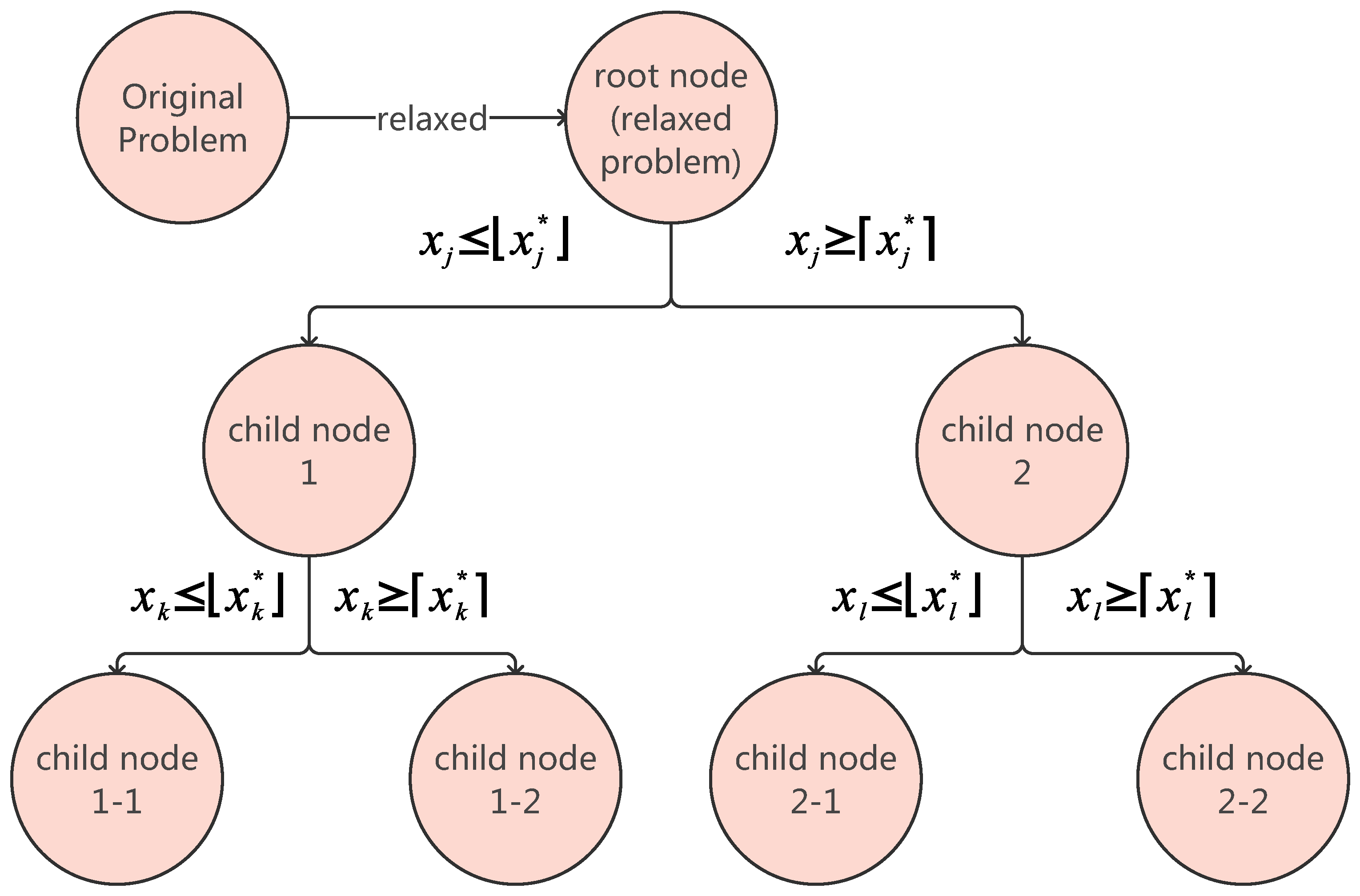
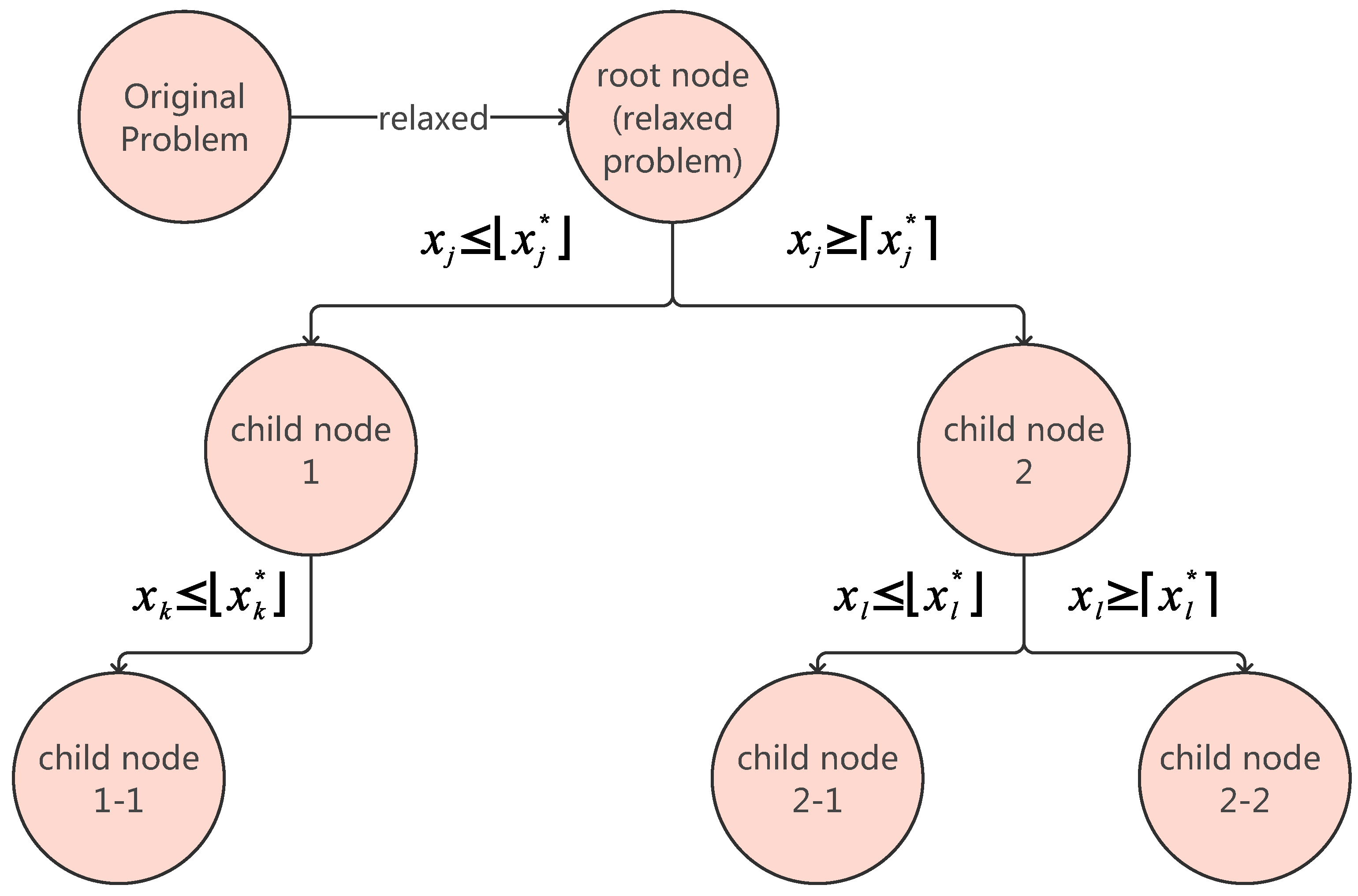
• Node: Based on the position of nodes in the search tree, they can be categorized into root nodes and child nodes. Based on the relationships between nodes, they are classified as parent nodes and child nodes. For example, child node 1 serves as the parent node for child nodes 1-1 and 1-2. Each node represents a constrained subproblem of the original problem, containing a constraint set, a relaxed solution, and status indicators. The constraint set inherits constraints from its parent node and adds new branching constraints. For instance, the constraint set of child node 1 includes constraints from the root node as well as the newly added constraint $x_j\le \lfloor x_j^{*}\rfloor$. Here, $\lfloor x\rfloor$ denotes the floor function of x, e.g., $\lfloor 4.81\rfloor =4$.
• Status indicators: These are used to denote the state of a node, categorized as unexplored or explored. Branching, pruning, or requiring no action will change the node’s status from unexplored to explored. Requiring no action indicates that the relaxed solution of the current node is an integer solution, and its objective value exceeds the current $LB$.
• Branching: Here, one selects a non-integer variable $x_j^{*}$ to partition the solution space into two branches: $x_j\le \lfloor x_j^{*}\rfloor$ and $x_j\ge \lceil x_j^{*}\rceil$. For example, the root node is divided into child node 1 and child node 2. Here, $\lceil x\rceil$ denotes the ceiling function of x, e.g., $\lceil 1.57\rceil =2$.
• Pruning: Subsequent branching operations are halted at the node. As illustrated in Figure 3, pruning removes child node 1-2 from the search tree. Pruning is justified under two conditions: (1) the relaxed solution is infeasible, or (2) the node’s upper bound satisfies $U{B}_i\le LB$ (e.g., $U{B}_i=327\le LB=340$). Here, $U{B}_i$ represents the relaxed solution value of node i.
• Search Tree: This is hierarchical node collection with root–child relationships.

The algorithm iteratively executes branching, bounding, and pruning until convergence. For example, branching at root node creates child nodes 1 and 2, whose union preserves all integer solutions while reducing the search space. Subsequent bound updates and pruning operations progressively tighten the solution envelope, ultimately yielding the global optimum when $UB$ and $LB$ coincide.

To elucidate the branch-and-bound algorithm workflow, we analyzed an integer linear programming (ILP) instance. Note that ILP constitutes a special case of mixed-integer programming (MIP), where all decision variables must be integers. Consider the following ILP problem:

$$\begin{array}{c}\max Z=40x_1+90x_2\end{array}$$

(45)

$$\begin{array}{c}\mathrm{such} \mathrm{that}9x_1+7x_2\le 56\end{array}$$

(46)

$$\begin{array}{c}7x_1+20x_2\le 70\end{array}$$

(47)

$$\begin{array}{c}{x}_1,x_2\ge 0\end{array}$$

(48)

$$\begin{array}{c}{x}_1,x_2\in {\mathbb{Z}}^{+}.\end{array}$$

(49)

Its linear programming relaxation becomes

$$\begin{array}{c}\max Z=40x_1+90x_2\end{array}$$

(50)

$$\begin{array}{c}\mathrm{such} \mathrm{that}9x_1+7x_2\le 56\end{array}$$

(51)

$$\begin{array}{c}7x_1+20x_2\le 70\end{array}$$

(52)

$$\begin{array}{c}{x}_1,x_2\ge 0.\end{array}$$

(53)

Solving the relaxation yields $(x_1,x_2)=(4.81,1.82)$ with $Z=356$ (initial upper bound). The feasible integer solution $(0,0)$ provides the initial lower bound $Z=0$.

• First Branching Operation
  • Branching Variable: $x_1=4.81$ (non-integer)
  • Child Node Generation:

    −

    Node 1 ($x_1\le 4$): Add constraint $x_1\le 4$, relaxed solution $(4,2.1)$ with $Z=349$

    −

    Node 2 ($x_1\ge 5$): Add constraint $x_1\ge 5$, relaxed solution $(5,1.57)$ with $Z=341$

  • Bound Update:

    −

    Upper Bound (UB): $\max (349,341)=349$

    −

    Lower Bound (LB): Remains 0 (no integer solution found)

• Second Branching Operation
  • Branching Variable: $x_2=2.1$ (non-integer)
  • Child Node Generation:

    −

    Node 1-1 ($x_2\le 2$): Add constraint $x_2\le 2$, integer solution $(4,2)$ with $Z=340$

    −

    Node 1-2 ($x_2\ge 3$): Add constraint $x_2\ge 3$, infeasible solution $(1.42,3)$ with $Z=327$

  • Bound Update:

    −

    Lower Bound (LB): $\max (0,340)=340$

    −

    Upper Bound (UB): $\max (341,327)=341$

  • Pruning:

    −

    Node 1-2 pruned (Rule: Bound), since $327<340$

• Third Branching Operation
  • Branching Variable: $x_2=1.57$ (non-integer)
  • Child Node Generation:

    −

    Node 2-1 ($x_2\le 1$): Add constraint $x_2\le 1$, solution $(5.44,1)$ with $Z=308$

    −

    Node 2-2 ($x_2\ge 2$): Infeasible

  • Pruning:

    −

    Node 2-1 pruned (Rule: Bound), since $308<340$

    −

    Node 2-2 pruned (Rule: Infeasibility)

• Algorithm Termination
  • All active nodes processed
  • Final Solution:

    −

    Optimal integer solution: $(x_1,x_2)=(4,2)$

    −

    Objective value: $LB=UB=340$

The branch-and-bound algorithm pseudo-code is formalized in Algorithm 1.

Algorithm 1. Branch-and-Bound Algorithm for Site Selection Problem

Input: Integer linear programming problem: $\max {\mathbf{c}}^T\mathbf{x},A\mathbf{x}\le \mathbf{b},\mathbf{x}\in {\mathbb{Z}}_{\ge 0}^d$ Output: Optimal solution ${\mathbf{x}}^{*}$, optimal value $Z^{*}$

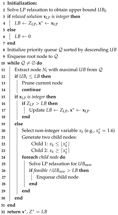
4. Simulation Results

The numerical experiments were conducted on a MacBook Pro equipped with a 3.5 GHz M2 Pro chip and 16 GB RAM. Additionally, we compared our approach with an existing station placement scheme [22] (denoted as the “existing method”), which can be summarized as follows: Under a single GEO satellite scenario, it minimizes the GS construction cost while satisfying the system availability (SA) constraints. The system availability is defined as the probability that at least one satellite-to-ground link remains operational. For instance, consider a satellite–ground laser communication system comprising three GSs and one GEO satellite. If the availability probabilities of the three satellite-to-ground links during a specific period are $\{0.6,0.7,0.8\}$, the system availability is calculated as $1-(1-0.6)\times (1-0.7)\times (1-0.8)=97.6\%$.

The comparative experimental procedure is as follows: The existing method outputs GS placement information and the associated cost. Based on the placement information, we solve the satellite-to-ground laser link scheduling problem to determine the system throughput under that placement configuration. The cost from the existing method serves as an input to our proposed placement model, which directly outputs the system throughput for comparison with the existing method. This ensures a fair throughput comparison between different placement schemes under identical cost constraints. Specific simulation parameters are configured as follows: We assume the number of time periods $T=24$, with each period lasting 1 h. The number of LEO satellites is 20. The transmission rate between GEO satellites and GSs is fixed at 1 Gb/s, while the transmission rate between LEO satellites and GSs is fixed at 30 Gb/s. The availability probability of LEO satellites to GSs during any time period follows a uniform distribution over $[0,1]$. Additionally, the base installation cost is defined as $c_g^{\mathrm{base}}=\lceil g/5\rceil$ for $g\in G$, where $\lceil x\rceil$ denotes the ceiling operation.

4.1. Data Throughput Comparison Under Different System Availability Constraints

In this section, we compare the data throughput under different system availability constraints. We set the number of candidate GSs at $G=25$. For each time period, the availability probability of the GEO satellite to different GSs follows a uniform distribution over $[0.25,0.75]$, denoted as $p_{t,g}^{avb}\sim U(0.25,0.75)$. The marginal cost per additional LCT $C_{LCT}=2$.

Figure 4 illustrates the throughput comparison under different station placement schemes, assuming the satellite–ground laser communication system contains 20 LEO satellites. Since the existing method only considers scenarios where each GS is equipped with a single LCT (laser communication terminal), for fairness in throughput comparison, our proposed scheme is divided into two configurations: $Q=1$ (fixed deployment) and Q as a variable (denoted as $Q_{\mathrm{var}}$ in the figure). Specifically, when Q is variable, we assume $C_{\mathrm{LCT}}=2$, indicating a cost increase of 2 for each additional LCT installed at a GS.

As shown in Figure 4, the proposed placement scheme achieves higher throughput than the existing method. This is because the existing method primarily considers GEO-to-GS availability probabilities during placement, while the system throughput includes contributions from both LEO–ground and GEO–ground laser links. The existing method lacks comprehensive temporal consideration of LEO–ground laser links, which exhibit significantly higher transmission rates (30 Gb/s). This omission leads to suboptimal throughput performance compared to our proposed scheme, which accounts for both link types across all time periods.

Further, comparing fixed deployment ($Q=1$, i.e., one LCT per GS) and dynamic deployment ($Q_{\mathrm{var}}$, $C_{\mathrm{LCT}}=2$, $L_{\mathrm{up}}=3$), the dynamic scheme optimizes LCT allocation under the cost constraint ${\sum }_{g=1}^G\left[c_g^{\mathrm{base}}+C_{\mathrm{LCT}}(Q-1)\right]z_g\le C_{\mathrm{up}}$. It prioritizes deploying multiple LCTs at GSs with superior communication conditions (i.e., higher data transmission potential). Although this reduces the total number of deployed GSs, it enhances the density of high-availability links. By maintaining an equivalent link scale while improving link quality, the dynamic scheme achieves throughput performance comparable to or better than the fixed deployment. Theoretically, the solution space of the dynamic scheme strictly encompasses that of the fixed scheme, ensuring inherent superiority in its optimal solution.

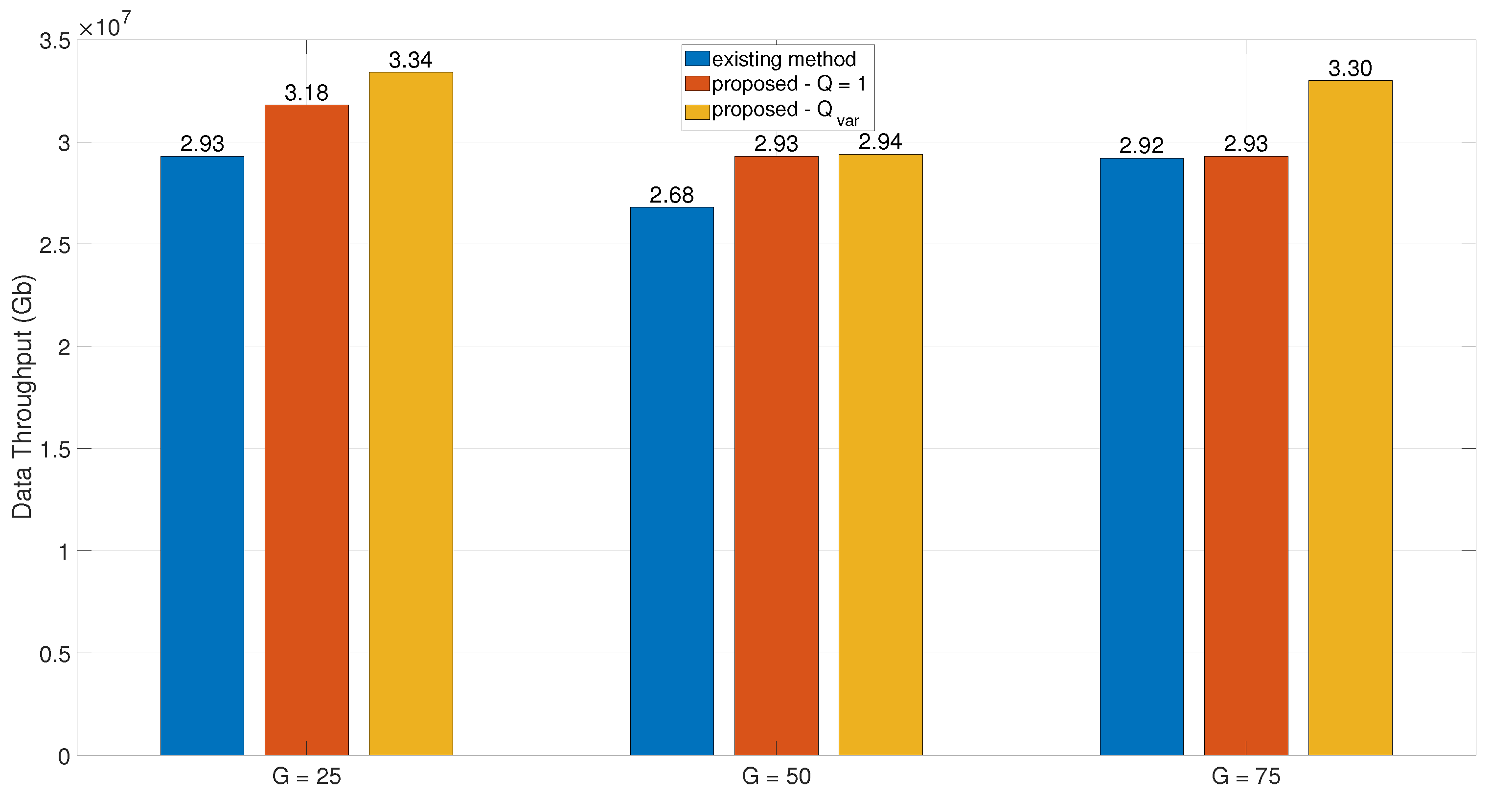
4.2. Data Throughput Comparison Under Different Number of Candidate GSs

In this section, we compare the data throughput under different number of candidate GSs. We set the number of candidate GSs ranging between 25 to 75. For each time period, the availability probability of the GEO satellite to different GSs follows a uniform distribution over $[0.25,0.75]$. The system availability constraint of the existing method is 0.999. The marginal cost per additional LCT $C_{LCT}=2$.

As demonstrated in Figure 5, the proposed site selection framework consistently outperforms existing methods in terms of data throughput across varying numbers of candidate GSs. Notably, the dynamic LCT deployment scheme ($Q_{var}$) exhibits superior performance compared to the fixed-LCT configuration ($Q=1$), validating the effectiveness of integer-scaled LCT allocation under cost constraints. While increasing the candidate GS pool size (in other words, number of GSs) intuitively expands spatial diversity for satellite–ground connectivity, our analysis reveals a non-monotonic relationship between GS quantity and data throughput enhancement. This phenomenon arises from the fundamental trade-off governed by the proposed joint optimization framework: system throughput depends not merely on the number of deployed GSs but holistically on the interplay between laser link availability probabilities ($p_{t,s,g}^{avb}$), transmission rates (${\varphi }_{t,s,g}$), and cost-constrained resource allocation.

The throughput saturation observed at larger GS pool sizes stems from two critical factors. First, under the uniform distribution assumption for link availability probabilities ($p_{t,g}^{avb}\sim U[0.25,0.75]$), the stochastic nature of cloud-induced outages inherently limits the exploration space for optimal downlink scheduling. Second, the linear cost model $c_g\left(Q\right)=c_g^{base}+C_{LCT}(Q-1)$ imposes strict budgetary boundaries, prioritizing quality (high $p_{t,g}^{avb}$) over quantity when expanding GS deployments.

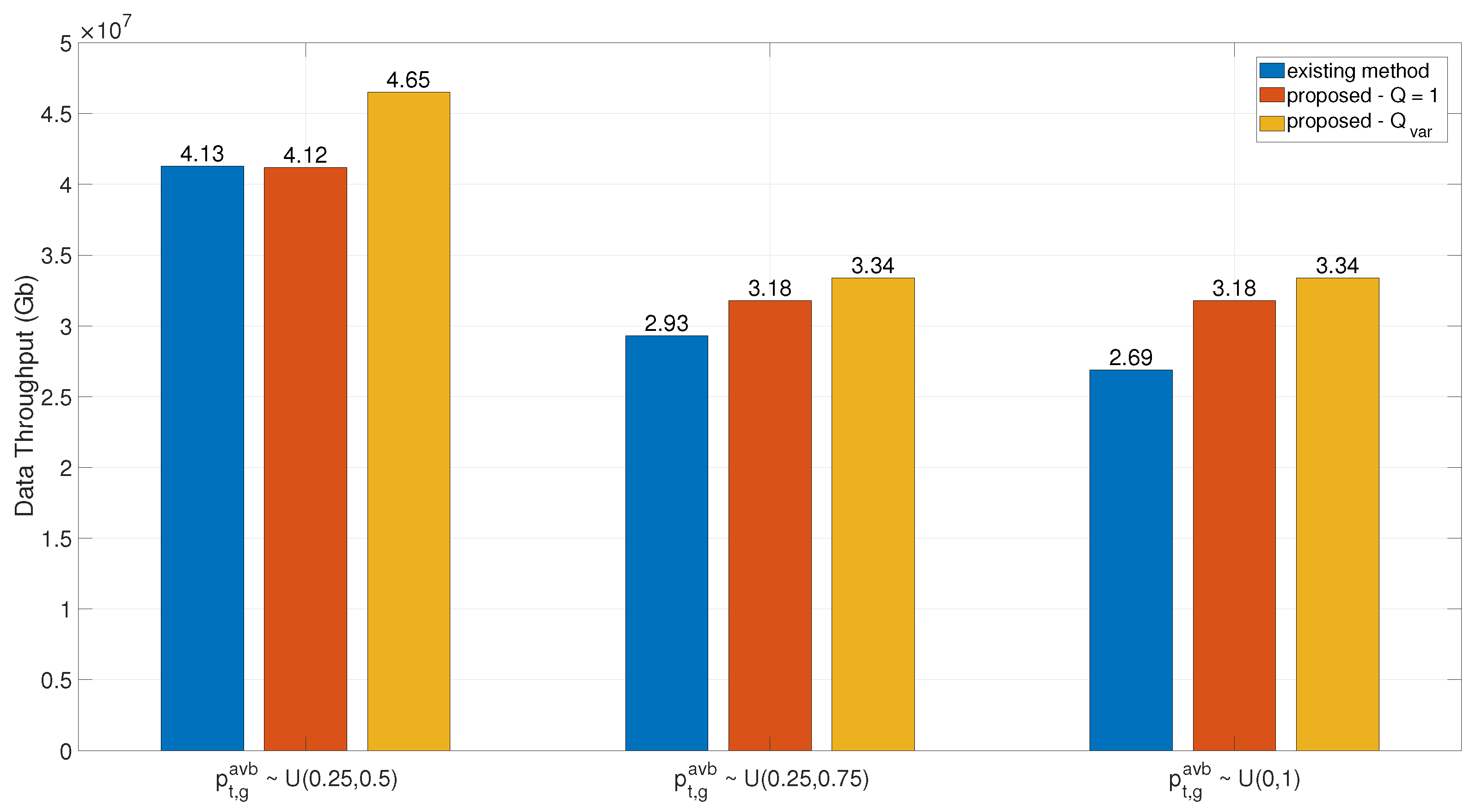
4.3. Data Throughput Comparison Under Different Distributions of Link Availability Probability

In this section, we compare the data throughput under different distributions of link availability probability. We set the number of candidate GSs to 25. For each time period, the availability probability of the GEO satellite to different GSs follows a uniform distribution over $[0.25,0.5]$, $[0.25,0.75]$, and $[0,1]$, respectively. The system availability constraint of the existing method is 0.999. The marginal cost per additional LCT $C_{LCT}=2$.

As shown in Figure 6, when the link availability probability obeys $Usim(0.25,0.5)$, all the compared methods achieve the highest data throughput across three distinct distributions. This is because the lower availability probability necessitates selecting more GSs to satisfy the system availability constraints, thereby relaxing cost constraints and enabling our proposed method to identify optimal solutions within an expanded solution space. Figure 6 also demonstrates that the system exhibits comparable data throughput performance under different link availability probability distributions (e.g., uniform distributions $U\sim (0,1)$ vs. $U\sim (0.5,0.75)$). This convergence stems from the synergistic interplay of multiple optimization mechanisms: while the $U\sim (0,1)$ distribution inherently includes low-probability links ($p_{t,g}^{avb}<0.5$), the proposed optimization framework inherently filters out such low-quality connections through its downlink scheduling mechanism. Specifically, the model prioritizes GSs with high availability probabilities ($p_{t,g}^{avb}>0.5$), leading to an activated GS subset that largely overlaps with the high-probability candidate pool under the $U\sim (0.5,0.75)$ distribution.

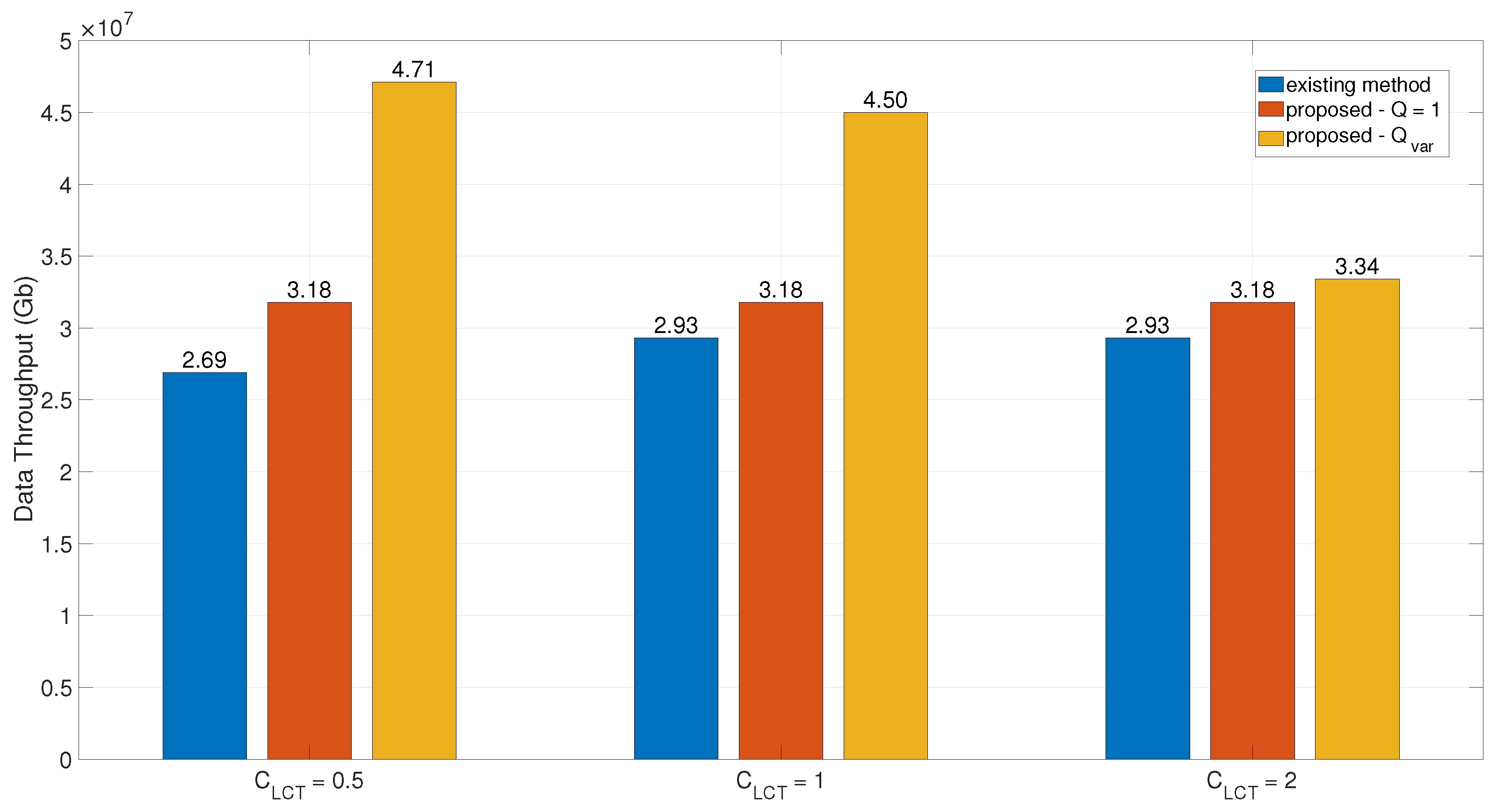
4.4. Data Throughput Comparison Under Different Marginal Costs per Additional LCT

In this section, we compare the data throughput under different $C_{LCT}$. The number of candidate GSs is 25. We set the number of candidate GSs 25. For each time period, the availability probability of the GEO satellite to different GSs follows a uniform distribution over $[0.25,0.75]$. The system availability constraint of the existing method is 0.999. The marginal cost per additional LCT $C_{LCT}\in \{0.5,1,2\}$.

It can be observed from Figure 7 that the increase in the marginal cost of LCT, $C_{LCT}$, leads to reduced throughput in the dynamic deployment scheme (Q-variable) due to the cost-constrained trade-offs in resource allocation. Under the optimization model, the total deployment cost is bounded by the budget $C_{up}$, expressed as ${\sum }_g\left[c_g^{base}+C_{LCT}(Q-1)\right]z_g\le C_{up}$. As $C_{LCT}$ rises, the higher per-unit cost of additional LCTs forces the model to compromise in two critical dimensions. First, fewer LCTs are deployed per GS (reduced Q values) to adhere to the cost constraint, directly diminishing the concurrent link capacity of individual GSs and limiting their ability to exploit time windows of high-availability links. Second, maintaining higher Q values necessitates reducing the total number of deployed GSs (fewer $z_g=1$), sacrificing spatial diversity gains. Even if the remaining GSs exhibit superior link quality, the reduced GS count restricts opportunities for satellites to dynamically select optimal links during scheduling. Furthermore, elevated $C_{LCT}$ undermines the model’s flexibility to balance “quality” (prioritizing multi-LCT deployments at high-availability stations) against “quantity” (deploying more stations with fewer LCTs). Consequently, the inherent advantage of dynamic LCT deployment—targeted resource concentration at favorable sites—is constrained, leading to suboptimal throughput due to reduced concurrent link density and diminished scheduling flexibility.

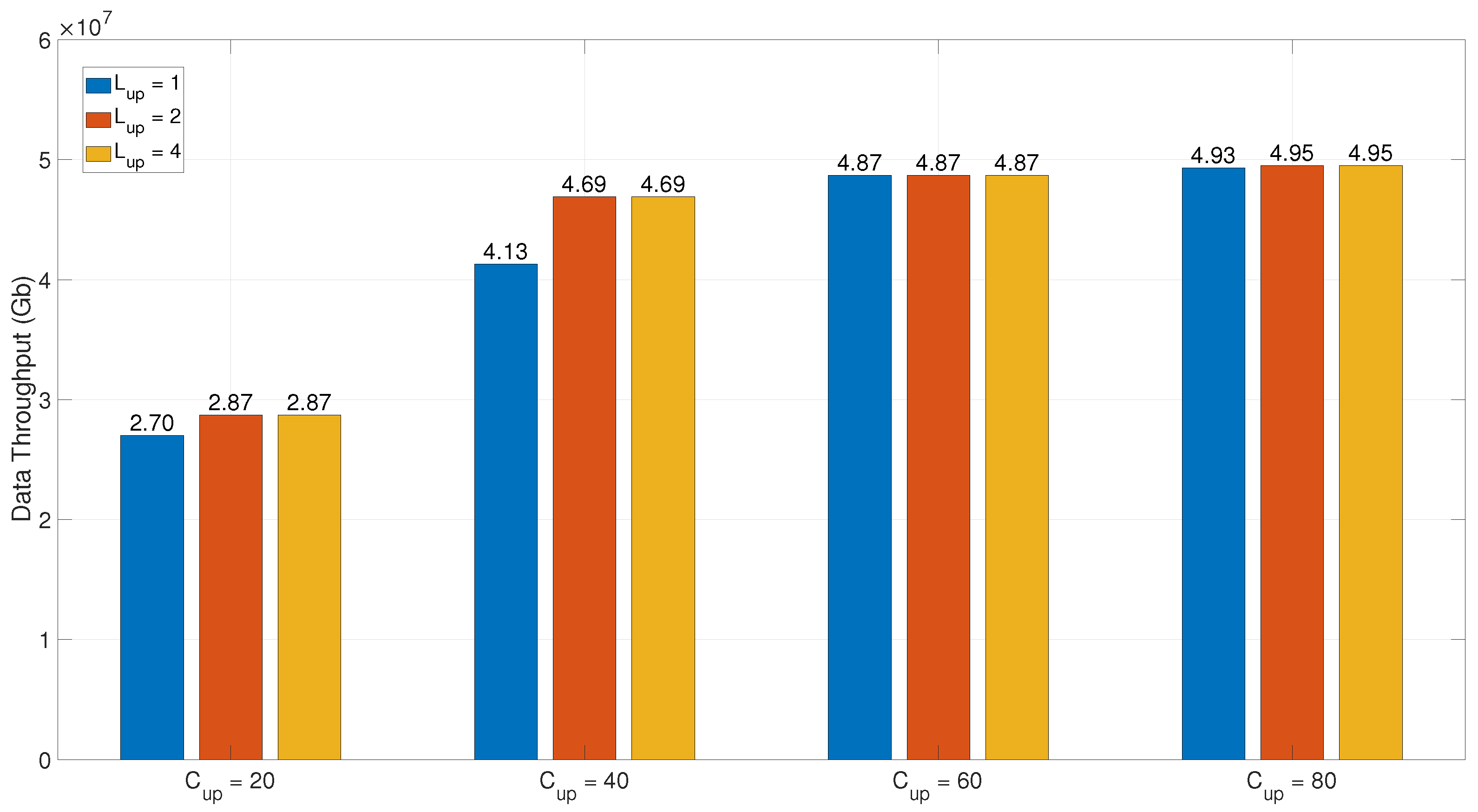
4.5. Impact of Cost Upper Limit on Data Throughput

Figure 8 further reveals the regulatory mechanism of the construction cost upper limit $C_{\mathrm{up}}$ on system data throughput. Similarly, the number of candidate GSs is 25. For each time period, the availability probability of the GEO satellite to different GSs follows a uniform distribution over $[0.25,0.75]$. The marginal cost per additional LCT $C_{LCT}=2$. It can be seen from Figure 8 that as $C_{\mathrm{up}}$ increases, the relaxed cost constraint allows more high-cost GSs to be incorporated into the candidate set, thereby enhancing the spatiotemporal coverage capability of satellite–ground links. Notably, the optimal throughput for $L_{\mathrm{up}}=2$ and $L_{\mathrm{up}}=3$ completely coincide, indicating that under the current parameter configuration, the model’s optimal solution already saturates at $L_{\mathrm{up}}=2$. This phenomenon can be explained as follows: When the per-station LCT upper limit increases to 3, the marginal throughput gain from incremental deployments fails to offset the associated construction cost increments. Consequently, the actual number of LCTs deployed in the optimal solution remains constrained by the cost–benefit equilibrium point, rendering further relaxation of the $L_{\mathrm{up}}$ constraint ineffective in altering the optimal decision.

5. Conclusions

This study establishes a data throughput-centric optimization paradigm that fundamentally advances GS site selection for SGLC systems. By synergistically combining downlink scheduling dynamics with site selection decisions—a critical integration absent in conventional approaches—the proposed framework enables precise evaluation of candidate sites’ data throughput capabilities. The introduction of an integer-scaled LCT deployment variable Q effectively balances the infrastructure costs with operational capacity, while the transformation of nonlinear constraints into an ILP formulation through auxiliary variable linearization ensures computational tractability. The branch-and-bound algorithm guarantees globally optimal solutions by systematically navigating the combinatorial search space. Numerical simulations demonstrate superior data throughput performance over existing solutions under equivalent installation cost constraints. Future extensions will incorporate multi-objective trade-offs and probabilistic weather correlation models to further refine operational robustness and investigate the impact of transient atmospheric phenomena (e.g., turbulence-induced fading, precipitation attenuation) on site selection and downlink scheduling.

References

1. Li, X.; Fan, F.; Yu, H.; Wang, Y.; Dai, X.; Yang, Q.; Liu, R. A Bidirectional Multi-Format/Rate-Adjustable Integrated Laser Communication System for Satellite Communication. IEEE Photonics J. 2024, 16, 1–6. [Google Scholar] [CrossRef]
2. Liang, J.; Chaudhry, A.U.; Erdogan, E.; Yanikomeroglu, H.; Kurt, G.K.; Hu, P.; Ahmed, K.; Martel, S. Free-Space Optical (FSO) Satellite Networks Performance Analysis: Transmission Power, Latency, and Outage Probability. IEEE Open J. Veh. Technol. 2024, 5, 244–261. [Google Scholar] [CrossRef]
3. Guelman, M.; Kogan, A.; Kazarian, A.; Livne, A.; Orenstein, M.; Michalik, H. Acquisition and pointing control for inter-satellite laser communications. IEEE Trans. Aerosp. Electron. Syst. 2004, 40, 1239–1248. [Google Scholar] [CrossRef]
4. Li, M.; Hong, Y.; Zeng, C.; Song, Y.; Zhang, X. Investigation on the UAV-To-Satellite Optical Communication Systems. IEEE J. Sel. Areas Commun. 2018, 36, 2128–2138. [Google Scholar] [CrossRef]
5. Bushuev, D.; Kedar, D.; Arnon, S. Analyzing the performance of a nanosatellite cluster-detector array receiver for laser communication. J. Light. Technol. 2003, 21, 447–455. [Google Scholar] [CrossRef]
6. Arnon, S.; Rotman, S.; Kopeika, N. Bandwidth maximization for satellite laser communication. IEEE Trans. Aerosp. Electron. Syst. 1999, 35, 675–682. [Google Scholar] [CrossRef]
7. Al-Hraishawi, H.; Chougrani, H.; Kisseleff, S.; Lagunas, E.; Chatzinotas, S. A Survey on Nongeostationary Satellite Systems: The Communication Perspective. IEEE Commun. Surv. Tutor. 2023, 25, 101–132. [Google Scholar] [CrossRef]
8. Xie, W.; Tan, L.; Ma, J. Received Signal Strength Reduction Analysis Based on the Wavelet Model in Intersatellite Laser Communications. J. Light. Technol. 2011, 29, 2327–2332. [Google Scholar] [CrossRef]
9. Dang, K.D.; Le, H.D.; Nguyen, C.T.; Pham, A.T. Resource allocation for hybrid FSO/RF satellite-assisted multiple backhauled UAVs over Starlink networks. IEICE Commun. Express 2024, 13, 52–55. [Google Scholar] [CrossRef]
10. Zedini, E.; Kammoun, A.; Alouini, M.S. Performance of Multibeam Very High Throughput Satellite Systems Based on FSO Feeder Links With HPA Nonlinearity. IEEE Trans. Wirel. Commun. 2020, 19, 5908–5923. [Google Scholar] [CrossRef]
11. Samy, R.; Yang, H.C.; Rakia, T.; Alouini, M.S. Hybrid SAG-FSO/SH-FSO/RF Transmission for Next-Generation Satellite Communication Systems. IEEE Trans. Veh. Technol. 2023, 72, 14255–14267. [Google Scholar] [CrossRef]
12. Le, H.D.; Trinh, P.V.; Pham, T.V.; Kolev, D.R.; Carrasco-Casado, A.; Kubo-Oka, T.; Toyoshima, M.; Pham, A.T. Throughput Analysis for TCP Over the FSO-Based Satellite-Assisted Internet of Vehicles. IEEE Trans. Veh. Technol. 2022, 71, 1875–1890. [Google Scholar] [CrossRef]
13. Spangelo, S.C.; Cutler, J.W.; Klesh, A.T.; Boone, D.R. Models and Tools to Evaluate Space Communication Network Capacity. IEEE Trans. Aerosp. Electron. Syst. 2012, 48, 2387–2404. [Google Scholar] [CrossRef]
14. Gong, S.; Shen, H.; Zhao, K.; Li, W.; Zhou, H.; Wang, R.; Sun, Z.; Zhang, X. Toward Optimized Network Capacity in Emerging Integrated Terrestrial-Satellite Networks. IEEE Trans. Aerosp. Electron. Syst. 2020, 56, 263–275. [Google Scholar] [CrossRef]
15. Spangelo, S.; Cutler, J.; Gilson, K.; Cohn, A. Optimization-based scheduling for the single-satellite, multi-ground station communication problem. Comput. Oper. Res. 2015, 57, 1–16. [Google Scholar]
16. Lyras, N.K.; Efrem, C.N.; Kourogiorgas, C.I.; Panagopoulos, A.D.; Arapoglou, P.D. Optimizing the Ground Network of Optical MEO Satellite Communication Systems. IEEE Syst. J. 2020, 14, 3968–3976. [Google Scholar] [CrossRef]
17. Lyras, N.K.; Efrem, C.N.; Kourogiorgas, C.I.; Panagopoulos, A.D. Optimum Monthly Based Selection of Ground Stations for Optical Satellite Networks. IEEE Commun. Lett. 2018, 22, 1192–1195. [Google Scholar] [CrossRef]
18. Fuchs, C.; Moll, F. Ground station network optimization for space-to-ground optical communication links. J. Opt. Commun. Netw. 2015, 7, 1148–1159. [Google Scholar] [CrossRef]
19. Poulenard, S.; Crosnier, M.; Rissons, A. Ground segment design for broadband geostationary satellite with optical feeder link. J. Opt. Commun. Netw. 2015, 7, 325–336. [Google Scholar] [CrossRef]
20. Gong, S.; Shen, H.; Zhao, K.; Wang, R.; Zhang, X.; De Cola, T.; Fraier, J.A. Network Availability Maximization for Free-Space Optical Satellite Communications. IEEE Wirel. Commun. Lett. 2020, 9, 411–415. [Google Scholar] [CrossRef]
21. Efrem, C.N.; Panagopoulos, A.D. Globally Optimal Selection of Ground Stations in Satellite Systems With Site Diversity. IEEE Wirel. Commun. Lett. 2020, 9, 1101–1104. [Google Scholar] [CrossRef]
22. Efrem, C.N.; Panagopoulos, A.D. Minimizing the Installation Cost of Ground Stations in Satellite Networks: Complexity, Dynamic Programming and Approximation Algorithm. IEEE Wirel. Commun. Lett. 2021, 10, 378–382. [Google Scholar] [CrossRef]
23. Alfa, A.S.; Maharaj, B.T.; Lall, S.; Pal, S. Mixed-integer programming based techniques for resource allocation in underlay cognitive radio networks: A survey. J. Commun. Netw. 2016, 18, 744–761. [Google Scholar] [CrossRef]
24. Jin, M.; Hu, R.Q.; Zhang, Z.; Hu, W. Integer linear programming models and performance evaluation on wavelength rearrangement in a mesh-restored all-optical network. IEEE Commun. Lett. 2006, 10, 111–113. [Google Scholar] [CrossRef]
25. Garau-Luis, J.J.; Torrens, S.A.; Vila, G.C.; Pachler, N.; Crawley, E.F.; Cameron, B.G. Frequency Plan Design for Multibeam Satellite Constellations Using Integer Linear Programming. IEEE Trans. Wirel. Commun. 2024, 23, 3312–3327. [Google Scholar] [CrossRef]
Figure 1. Schematic diagram of ground station site selection based on system availability: an SGLC system containing one GEO satellite and four candidate ground stations with a scheduling period of one time slot. Red and green bidirectional solid lines represent different site selection strategies.
Electronics 14 01479 g001
Figure 2. Example of node.
Electronics 14 01479 g002
Figure 3. Example of pruning.
Electronics 14 01479 g003
Figure 4. Data throughput comparison under different system availability constraints.
Electronics 14 01479 g004
Figure 5. Data throughput comparison under different number of candidate GSs.
Electronics 14 01479 g005
Figure 6. Data throughput comparison under different distribution of link availability probability.
Electronics 14 01479 g006
Figure 7. Data throughput comparison under different marginal costs per additional LCT.
Electronics 14 01479 g007
Figure 8. Impact of cost upper limit on data throughput.
Electronics 14 01479 g008
Disclaimer/Publisher’s Note: The statements, opinions and data contained in all publications are solely those of the individual author(s) and contributor(s) and not of MDPI and/or the editor(s). MDPI and/or the editor(s) disclaim responsibility for any injury to people or property resulting from any ideas, methods, instructions or products referred to in the content.