Article

Artificial Intelligence-Driven Optimal Charging Strategy for Electric Vehicles and Impacts on Electric Power Grid

Department of Electrical and Computer Engineering, The University of Texas at San Antonio, San Antonio, TX 78249, USA
*
Author to whom correspondence should be addressed.
Electronics 2025, 14(7), 1471; https://doi.org/10.3390/electronics14071471
Submission received: 16 February 2025 / Revised: 28 March 2025 / Accepted: 31 March 2025 / Published: 6 April 2025
(This article belongs to the Special Issue Recent Advances in Modeling and Control of Electric Energy Systems)

Abstract

:
Electric vehicles (EVs) play a crucial role in achieving sustainability goals, mitigating energy crises, and reducing air pollution. However, their rapid adoption poses significant challenges to the power grid, particularly during peak charging periods, necessitating advanced load management strategies. This study introduces an artificial intelligence (AI)-integrated optimal charging framework designed to facilitate fast charging and mitigate grid stress by smoothing the “duck curve”. Data from Caltech’s Adaptive Charging Network (ACN) at the National Aeronautics and Space Administration (NASA) Jet Propulsion Laboratory (JPL) site was collected and categorized into day and night patterns to predict charging duration based on key features, including start charging time and energy requested. The AI-driven charging strategy developed optimizes energy management, reduces peak loads, and alleviates grid strain. Additionally, the study evaluates the impact of integrating 1.5 million, 3 million, and 5 million EVs under various AI-based charging strategies, demonstrating the framework’s effectiveness in managing large-scale EV adoption. The peak power consumption reaches around 22,000 MW without EVs, 25,000 MW for 1.5 million EVs, 28,000 MW for 3 million EVs, and 35,000 MW for 5 million EVs without any charging strategy. By implementing an AI-driven optimal charging optimization strategy that considers both early charging and duck curve smoothing, the peak demand is reduced by approximately 16% for 1.5 million EVs, 21.43% for 3 million EVs, and 34.29% for 5 million EVs.

1. Introduction

Electric vehicles (EVs) are widely recognized as a key solution for reducing air pollution and promoting sustainable transportation. According to the U.S. Energy Information Administration, 3.3 million EVs were recorded in the U.S. in January 2024 [1], up from 2 million in 2022 and 1.3 million in 2021. The increasing number of EVs on the roads has resulted in greater complexity and variability in charging behaviors, driven by diverse user habits and inconsistent energy demands. Traditional demand response (DR) approaches primarily depend on inflexible, predetermined load-shifting strategies designed for large industrial or commercial users, often managed through centralized control by energy providers [2]. However, there is a mismatch between the dynamic, real-time characteristics of EV charging demands and the static, rigid framework of traditional DR approaches, underscoring the need for more intelligent, adaptive, and real-time DR strategies [3,4,5] to ensure grid stability, optimize energy distribution, and alleviate peak stress on the power grid caused by EV charging requests [6].
In response to this challenge, recent research has increasingly explored intelligent EV charging optimization strategies that consider system-wide grid impacts [7,8,9,10,11,12,13,14,15,16]. Furthermore, substantial progress has been made in artificial intelligence (AI)-based EV energy management systems [17,18,19,20] and the development of intelligent EV charging infrastructure [21,22], with the goal of delivering highly adaptive, scalable, and efficient charging solutions that improve overall grid performance. The AI-driven DR systems dynamically adjust EV charging schedules based on real-time grid conditions, energy availability, and predictive analysis [23]. Such strategies can enhance grid stability and reduce peak demand more effectively than traditional DR methods by optimizing charging patterns in alignment with energy generation trends. Specifically, they help mitigate the duck curve effect by synchronizing charging with periods of high energy output [24]. Although AI-driven strategies require substantial computational resources for training and real-time data processing, they offer long-term advantages in adaptability and efficiency. Once deployed, these strategies enable self-optimizing, automated decision-making processes that outperform static, rule-based DR systems in both speed and flexibility [19]. To minimize data integrity attacks within the EV charging control center, a fuzzy inference-based advanced attack recovery system effectively enhances security in the vehicle–grid system [25].
Machine learning (ML) and density functional theory play an important role in optimizing catalyst development for green hydrogen production, addressing efficiency and yield challenges [26]. The insights gained from ML-driven advancements in hydrogen production can directly impact EV charging strategies, particularly for hydrogen fuel cell EVs [27]. Additionally, recent studies have incorporated battery-centric parameters such as state of charge (SoC) and state of health (SoH) to improve scheduling precision and system reliability [28]. These considerations support more effective battery management, reduce degradation, and enable the early detection of faults—facilitating proactive control measures to maintain safe and efficient EV operation [29]. AI techniques have also been applied for various predictive tasks, including charging load forecasting [30,31,32,33,34,35,36], user behavior estimation [37], charging point occupancy prediction [38], and charging duration estimation [39,40]. In [41], a degradation knowledge transfer learning approach was used to estimate battery SOH accurately as compared to other artificial intelligence techniques.
Among these variables, charging duration remains a pivotal factor in EV charging management, as it depends on critical parameters such as requested energy, start time, end time, and power level. Daily fluctuations in energy demand, particularly during peak hours, make it essential to forecast and manage EV charging duration effectively. Therefore, striking a balance between fast charging and minimizing grid stress represents a key optimization challenge. Most of the existing literature either focuses on predictive modeling or employs optimization techniques in isolation (as summarized in Table 1).
This study proposes an AI-enhanced EV charging framework that combines prediction and optimization to improve load management and flatten the duck curve. The framework uses AI to predict EV charging duration from features like charging start time and energy demand. These predictions feed into an optimization algorithm to enhance system-wide efficiency. The impact of different levels of EV integration under various AI-based strategies is then analyzed to assess grid performance and stability.
The remainder of this paper is structured as follows: Section 2 presents the proposed methodology. Section 3 discusses the experimental results and findings. Section 4 offers concluding remarks and suggestions for future research directions.

2. Methods

The ACN dataset features real data on EV charging across three sites in California— the Jet Propulsion Laboratory (JPL), the California Institute of Technology (Caltech), and Office 1. Table 2 provides details about each site’s location, the number of electric vehicle supply equipment (EVSE) units—defined as EV charging stations—and the total number of EV charging sessions recorded between 2018 and 2021, based on publicly available sources. This research focuses on the JPL site, due to its significantly higher volume of EV charging sessions in comparison to the other two locations.

2.1. EV Charging Data Preprocessing

EV charging data collected from JPL charging sites include multiple features, such as connection time, disconnect charging time, done charging time, and energy requested (assumed to be equal to the energy delivered, measured in kilowatt-hours (kWh)). Based on these existing features, the following additional variables were calculated: charging duration in hours (h), charging occupancy (h), charging rate or power in kilowatts (kW), and start charging time (h). A detailed explanation of each feature is provided in Table 3.
The original dataset provided the “connection time” in a datetime format, “Sun, 24 Mar 2019 22:30:47 GMT”. The feature “start charging time” was calculated by extracting the time and normalizing it to a float number between 0 and 24. For example, 22:30:47 was normalized to 22.513. The JPL charging station type was classified as level 2; according to the U.S. Department of Transportation, the estimated charging time for fully depleted battery EVs is about 4–10 h, while for plug-in hybrid EVs, it is around 1–2 h [42]. Therefore, only sessions with charging durations ranging from 1 to 10 h were considered in this study. Additionally, the highest observed charging power was generally below 6.6 kW, with only a few exceptions. As a result, a charging power range of 2.5 to 6.6 kW was selected for analysis, consistent with the specifications of level 2 charging stations.
In this study, the sessions conducted during weekdays were considered, while weekends and national holidays were excluded due to their low session frequency and limited relevance to typical usage patterns. The maximum number of charging sessions was observed in October 2019, and the complete dataset from this month is illustrated in Figure 1. To ensure data stability, the peak session month and year were selected, and the final four days—exhibiting minimal variation in the number of charging sessions—were used for training. This helps with training a reliable model, while validation based on the remaining dataset enhances the model’s generalizability.

2.1.1. Spearman’s Correlation Coefficient

To examine the monotonic relationships between the float-type features presented in Table 2, Spearman’s correlation coefficients are calculated, as defined by (1),
ρ s c c = 1 6 b j 2 m   ( m 2 1 )
where
ρ s c c = Spearman’s correlation coefficient;
b j = difference between ranks of each pair of observations;
m = the number of observations or data points.
A ρ s c c of 1 indicates a perfect positive correlation, a ρ s c c of −1 indicates a perfect negative correlation, and a ρ s c c of 0 indicates no correlation.

2.1.2. Feature Selection

In this study, “start charging time” and “energy requested ( e i )” are selected as input features, while “charging duration” serves as the target (output) feature. Both input features are significant for predicting charging duration. The energy requested has a direct impact on duration, as greater energy demands typically result in longer charging sessions. Start charging time is also crucial, as it aligns with daily grid usage patterns, such as peak and off-peak hours (e.g., daytime vs. nighttime), which influence both the efficiency and length of the charging session due to variations in grid demand. For the ith charging session, charging duration ( d i ) is calculated by subtracting the done charging time ( t d i ) and the start charging time ( t s i ) as shown in (2),
d i = t d i t s i
where input feature e i depends on charging power ( r i ) and charging duration ( d i ), is defined by (3)
e i = r i d i .
If T is the actual starting time (in hours of the day), then t s c t i can be defined for the entire day by (4) to distinguish between daytime and nighttime charging behaviors,
t s c t i = 6   a m T < 6   p m ( D a y ) 6   a m > T 6   p m ( N i g h t ) .

2.2. Quality Control of Data

Data visualization methods are employed to examine the data distribution and detect any inconsistencies within the datasets. In this study, we utilize a violin plot for quality control, as it effectively highlights the distribution of data. The shape of the violin plot is created using Kernel Density Estimation (KDE), a method for estimating the probability density function of a random variable. KDE transforms the distribution of discrete data points into a smooth, continuous curve, as defined by (5) for a univariate variable x ,
g ^ x = 1 m h 2 π j = 1 m e 1 2 x x j h 2 ,
where g ^ x is estimated density function, m is number of data points, x j is individual data point, h = 1.06 σ m 1 / 5 is a bandwidth, a smoothing parameter, determined by Silverman’s rule of thumb, and σ is the standard deviation of the data.
The mean or average value ( μ ) of the dataset consisting of m samples is defined by (6)
μ = 1 m j = 1 m x i .
The median ( Μ ), defined as the middle value of a dataset in (7), is determined differently based on the number of observations. If m is odd, the median is the middle value; if m is even, it is the average of the two central values,
Μ = x m + 1 2 ,     if m is odd x m 2 + x m 2 + 1 2 ,       if m is even .

2.3. Artificial Intelligence Model

Four models were implemented in this study to predict charging duration, namely linear regression (LR), Gaussian mixture regression (GMR), random forest regression (RFR), and the feedforward fully connected artificial neural network (FFC-ANN). A comparison between these models in terms of model type, characteristics, ability to handle nonlinearity, training complexity, and scalability is presented in Table 4. The FFC-ANN is emphasized due to its superior performance in capturing complex nonlinear relationships in the data, higher accuracy in predictions, and scalability to handle large datasets. The selection of an ANN model is driven by its ability to effectively model non-sequential relationships within the given dataset, making them highly suitable for this problem. Furthermore, they provide efficient learning with less computational overhead than reinforcement learning approaches, ensuring faster training and easier implementation. This makes FFC-ANNs an ideal choice for this task where clear input–output mappings are crucial, and the data are non-sequential.

Feedforward Fully Connected ANN Model

In the FFC-ANN model, each neuron in each layer is fully connected to all the neurons in the next layer, as shown in Figure 2. The input matrix for m samples, combining two inputs e i and t s c t i , is represented by X   R m × 2 . It can be defined by (8),
X i = e 1 t s c t 1 e m t s c t m .
At L hidden layers, l = 1 ,   2 ,   L , it can be defined by (9),
q i ( l ) = h ( W l q i ( l 1 ) + b ( l ) ) ,
where q i ( 0 ) = X i , W l is the weight matrix for layer l , b l is the bias vector for layer l , and h is the activation function. The output layer generates final predictions of charging duration d ^ i , as indicated by (10) and (11),
d ^ i = W L q i ( L 1 ) + b ( L ) ,
d ^ i = W L h h ( W 1 X i + b 1 ) + b ( L 1 ) + b ( L ) .

2.4. Model Evaluation

During model implementation, the data were split into two parts based on (4), distinguishing between day and night patterns. Each of these datasets was then trained and tested using an 80% and 20% ratio, respectively, and normalized using min–max scaling. Model evaluation was conducted using metrics such as Mean Squared Error (MSE), Mean Absolute Error (MAE), and R-squared (R2), as defined in Equations (12)–(14). These metrics are essential for assessing the model’s performance in estimating charging duration. They are calculated based on the real values ( d i ) and predicted values ( d i ^ ) , with m representing the total number of samples as follows,
M S E = 1 m i = 1 m ( d i d i ^ ) 2 ,
M A E = 1 m i = 1 m ( d i d i ^ ) ,
R 2 = 1 1 m i = 1 m d i ^ d ¯ 2 1 m i = 1 m d i d ¯ 2 .
where d ¯ is the mean value of testing sample.

2.5. Optimization

Scheduling of the EV charging was achieved by controlling the charging rate in a session with different objective functions. The objective function U 1 was established by promoting charging as shown in (15).
U 1 = m i n t τ i ν t T r i ( t ,
where U 1 is a function of a vector r ^ = { r i 1 ,…, r i T , i ν } , ν is the set of EV charging sessions in a specific time period such as one day, the optimization horizon to solve problem is defined as τ = { 1 , 2 , 3 T } , T is the last element of the time series τ , and r is a charging rate in kW. By determining the charging rate r for a session i at a specific time, the system can determine if the EV will not be charged ( r i τ = 0 ), or charged with a specific rate ( 0 < r i r m a x ) , where r m a x is the maximum charging rate of a charging station. The charging rate also affects a load imposing to the power grid.
The objective function U2 was established to smooth the duck curve as shown in (16).
U 2 = min t τ d ^ t d ^ ( t 1 ) 2 ,
where d t represents California ISO’s net power demand at time t , which can be scaled up and down to the charging stations’ system capacity assuming residential usage will not change significantly. The variable d ^ ( t ) = d t + i ν r i t represents the justified power demand with scheduled EV charging.
The objective U3 can be considered as a linear combination of the difference between current time (t) and expected ending time (T), t T , as well as the charging rates r i ( t ) . The objective function U3 deploys different weights of the charging rate denoted as a function f ( t T i d i ^ ) in (17),
U 3 = m i n t τ i ν f t T i d i ^ r i t ,
where T i represents the done charging time specific to a session i , t T i is then normalized with its predicted charging duration, d i ^ , such that t T i d i ^ will be limited to the domain [−1 0]. Five different concave and mono-increasing weight functions were considered for f t T i d i ^ in U3, such as t T i d i ^ ,   e 2   t T i d i ^ 1 ,   log t T i d i ^ + 1.001 ,     ln t T i d i ^ + 1.01 ,     a n d   0.05 tan t T i d i ^ + π 2 + 1.01 .
As the ultimate goal was to schedule EV charging with both early charging and a smooth duck curve, a combination of the U2 and U3 objectives were constructed as U 4 , asv indicated in (18),
U 4 = 1 n U 3 u 3 + n U 2 u 2
where weight n is a percentage of the importance of a smooth duck curve, and 1 − n is the importance of charging efficiency; u 2 and u 3 are defined as the best values of the separate minimizations of U 2 and U 3 in the previous sessions.

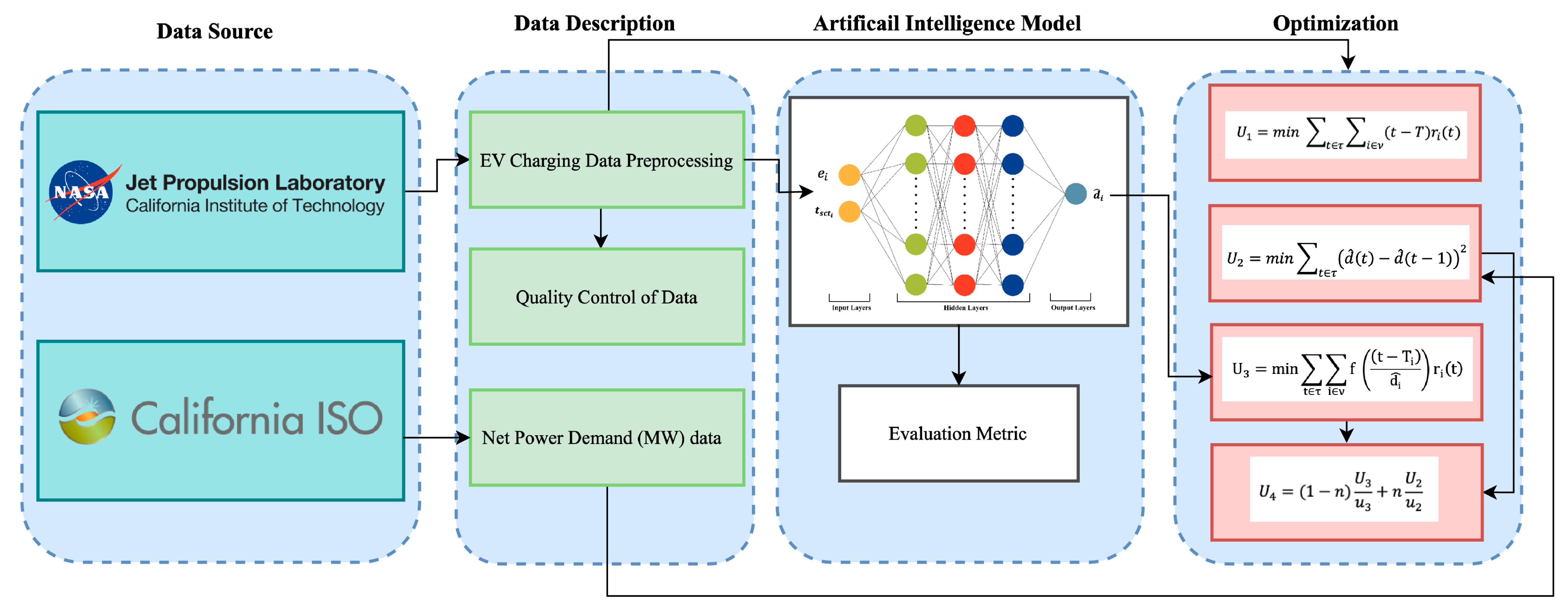
2.6. Computational Framework

Data preprocessing and AI model implementation for charging duration prediction were carried out using Jupyter Notebook 6.4.8, an open-source web-based interactive computational environment. The programming language utilized for this task is Python. 3.9.12 All simulations were executed on an AMD Ryzen 7 5800 8-Core Processor) (3.401 GHz) with 16 logical processors, using an Alienware system manufactured by Dell Technologies, headquartered in Round Rock, Texas, USA. Additionally, the optimization toolbox of MATLAB-R2024b was used to apply quadratic nonlinear programming functions for optimization purposes. The framework of the proposed research methodology is shown in Figure 3.

3. Results and Discussion

Section 3 has been divided into the following sub-sections:
(a)
Correlation analysis;
(b)
Data visualization for quality control;
(c)
Prediction of charging duration by FFC-ANN model;
(d)
Comparison of the FFC-ANN model with other AI models;
(e)
Optimization of power by different objective functions;
(f)
Impacts of EV integration on electric power grid.

3.1. Correlation Analysis

To examine the relationships among the various data features, Spearman’s correlation analysis was conducted, as shown in Figure 4. A correlation coefficient of 0.8761 was identified between the energy requested and charging duration, indicating a strong positive correlation. In contrast, a correlation coefficient of −0.2247 was found between the start charging time and the charging duration, suggesting a weak negative correlation. The features, energy requested and start charging time, were considered as input features, and used as the inputs to the AI models to predict charging duration, which was designated as the target or output feature.

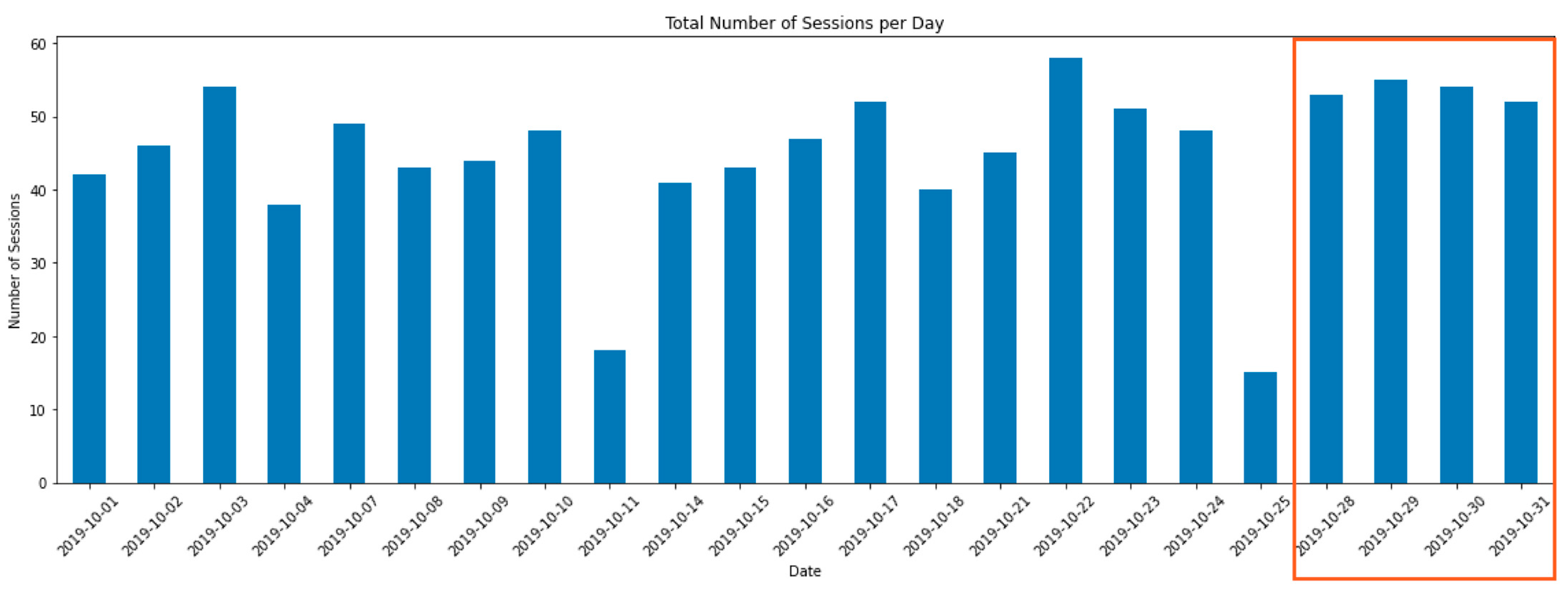
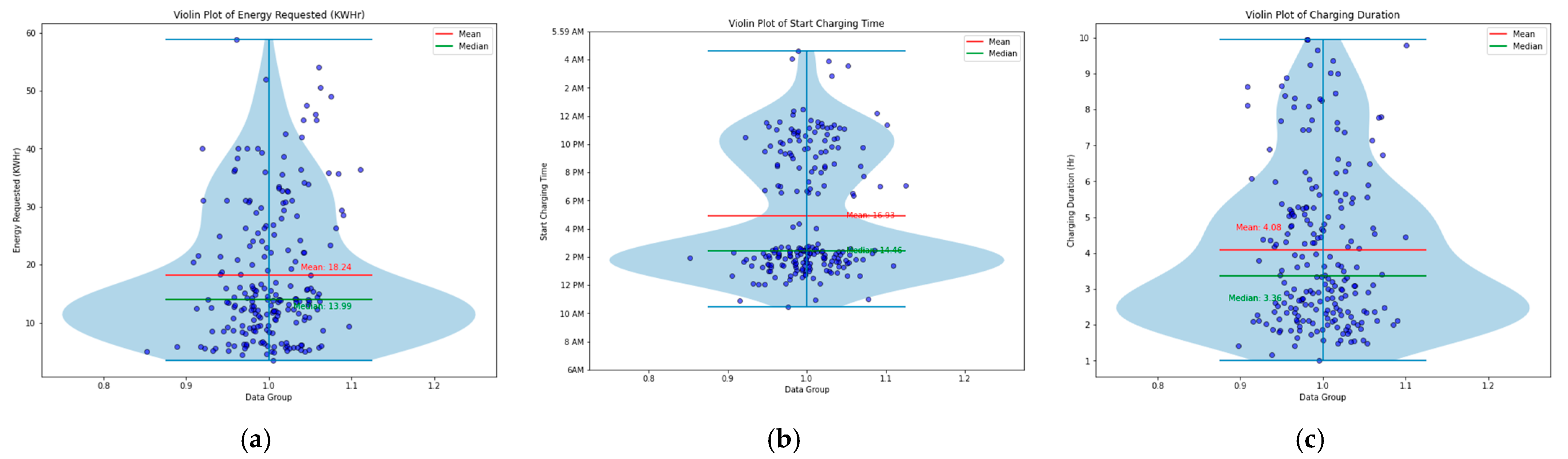
3.2. Data Visualization for Quality Control

Violin plots are used in data visualization to assess the distribution of data features, supporting quality control by identifying data trends, variability, and potential outliers. Figure 5a–c shows the distributions of both the input and output features. The violin plot for the energy requested input indicates mean and median values of 18.24 kWh and 13.99 kWh, respectively. For the start charging time input, the mean is 4:56 pm (16.93 h out of 24 h) and the median is 2:28 pm (14.46 h). In contrast, the mean and median values for charging duration as target feature for prediction are 4.08 h and 3.36 h, respectively. Interestingly, the start charging time feature showed a clear separation between daytime and nighttime, suggesting two different models for daytime and nighttime, respectively.

3.3. Prediction of Charging Duration by FFC-ANN Model

The artificial neural network (ANN) model was trained with various hyperparameters, including the number of neurons, learning rate, number of layers, epochs, and activation functions, for both the day ( 6   a m T < 6   p m ) and night ( 6   a m > T 6   p m ) datasets, as detailed in Table 5 and Table 6. Notably, the model’s performance improved with three hidden layers, as evidenced by the R2 scores achieved. Specifically, for the daytime dataset, the model attained an R2 score of 0.7189 with 50 layers, while the night dataset yielded R2 score of 0.8133. However, these scores were suboptimal compared to those achieved with 100 and 150 epochs.
As observed in Table 5 and Table 6, the hyperparameters at Sr. No. 12 and 13 demonstrated superior performance metrics and were thus selected for model training, as shown in Table 7. Given these hyperparameters for the subsequent experiments, a controlled environment was established to facilitate a clearer understanding of the model’s performance under consistent conditions. The mean R2 scores of 10 data partitions, randomly chosen from the selected four-day dataset, were 0.9348 for the day dataset and 0.8988 for the night dataset, using the fixed hyperparameters from serial number 13. The ANN model showed better performance on the nighttime dataset due to reduced variability and noise, as well as more predictable user behavior, allowing the model to capture stable patterns effectively.
The model was established with training datasets from 4 days, from 28 October to 31 October 2019. A total of 80% of the charging sessions were used for training and the remaining 20% were used for testing. The actual and predicted charging duration of the testing charging sessions are presented in Figure 6a and Figure 6b for the daytime and nighttime patterns, respectively.
Model validation was performed using 100 random samples from the non-training data (excluding the charging sessions from the 4 days used for training) for each data partition, as presented in Table 8. The mean value of R2 for the nighttime pattern is 0.9112, which is slightly higher than the mean value of 0.8816 for the daytime pattern. The evaluation metrics such as MSE, MAE, and R2 for 10 data partitions from the validation data for both day and night patterns are visualized in Figure 7a and Figure 7b, respectively. The MSE and MAE values in the daytime pattern are higher than in the nighttime pattern, suggesting a better performance of the nighttime model.

3.4. Comparison of the FFC-ANN Model with Other AI Models

The FFC-ANN model and other AI models, such as LR, GMR, and RFR, were compared using evaluation metrics such as MSE, MAE, and R2 across 10 different data partitions for daytime and nighttime patterns. The results for the LR, GMR, and RFR models are presented in Table 9, Table 10 and Table 11, while the FFC-ANN model’s findings are shown in Table 6.
Graphical representations of the mean values for these models are displayed in Figure 8a and Figure 8b, for the daytime and nighttime patterns, respectively. These results showed that the mean R2 values for the FFC-ANN model were higher, while the mean MSE and MAE were lower compared to the other AI models for both the daytime and nighttime patterns, suggesting good performance of the ANN model for this study. Therefore, the predicted charging duration obtained by the FFC-ANN model was integrated with defined objective functions for optimization.

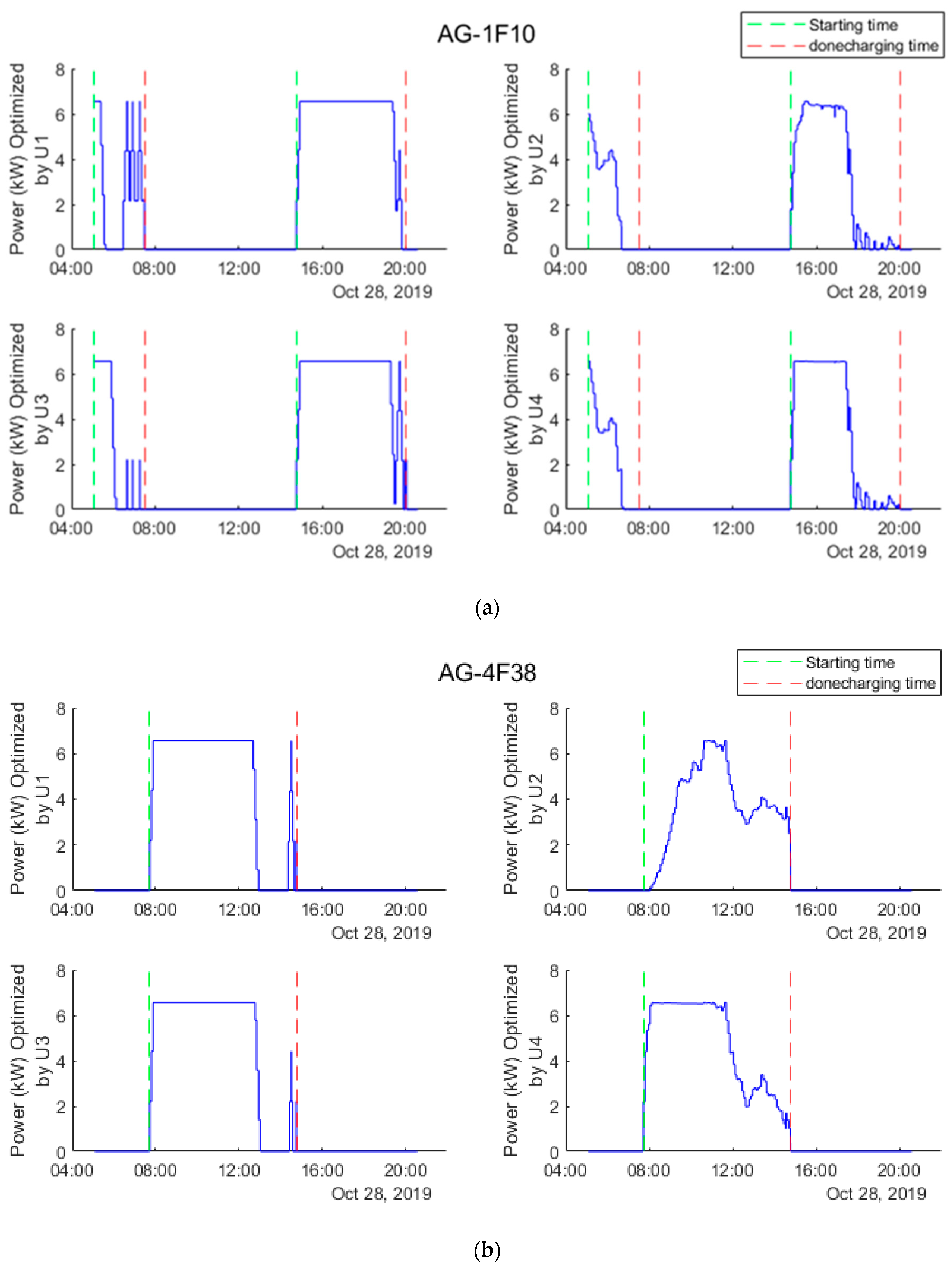
3.5. Optimization of Power by Different Objective Functions

Based on the time of training dataset, the scheduling for charging sessions on 28 October 2019 was used for optimization. The predicted charging durations from both the day and night patterns on this date were integrated into the third and fourth objective functions. The optimization process for the second and fourth objective functions utilized the net demand data sourced from the California Independent System Operator (ISO) [18] for the entire day. The patterns of these data are shown in Figure 9.
The system demand trend, measured in megawatts, was compared with forecasted demand in 5 min intervals. The net demand trend, defined as system demand minus wind and solar, was also presented in 5 min increments, compared to the total system to forecast demand, and used for optimization.
The optimization of the charging strategy was assessed by applying the optimized power data to each individual charging station. Figure 10a and Figure 10b display the optimized power results (in kW) for station IDs AG-1F10 and AG-4F3, respectively, across objective functions U1, U2, U3, and U4. The results indicated that objective function U4 demonstrated superior performance by achieving faster or earlier charging completion and contributing to a smoother duck curve. Additionally, U2 was effective in smoothing the duck curve, while U3 prioritized early charging. Practitioners can balance different objective weightings based on operational priorities, such as faster charging or smoother duck curve, as shown in objective function U4.
Three charging sessions were selected, with two sessions from the AG-1F10 charging station, charging duration from 5AM to 8AM, as well as from 3PM to 8PM, respectively, and one session from the AG-4F38 charging station from 8AM to 3PM. These three sessions represented a possible charging window from 4AM to 8PM within a single day. It was observed that linear optimization strategy, with U1 as the objective function, showed spikes in power demand near the end of the charging duration. The charging strategy with U3 demonstrated earlier charging activities with reduced end-of-session spikes for all three selected charging sessions. The charging strategy with U2 as the objective function resulted in a smooth power demand curve without end-of-session spikes, although minor fluctuations may still be present. The charging strategy using U4 achieved both a smooth power profile and an earlier completion of most charging demands.

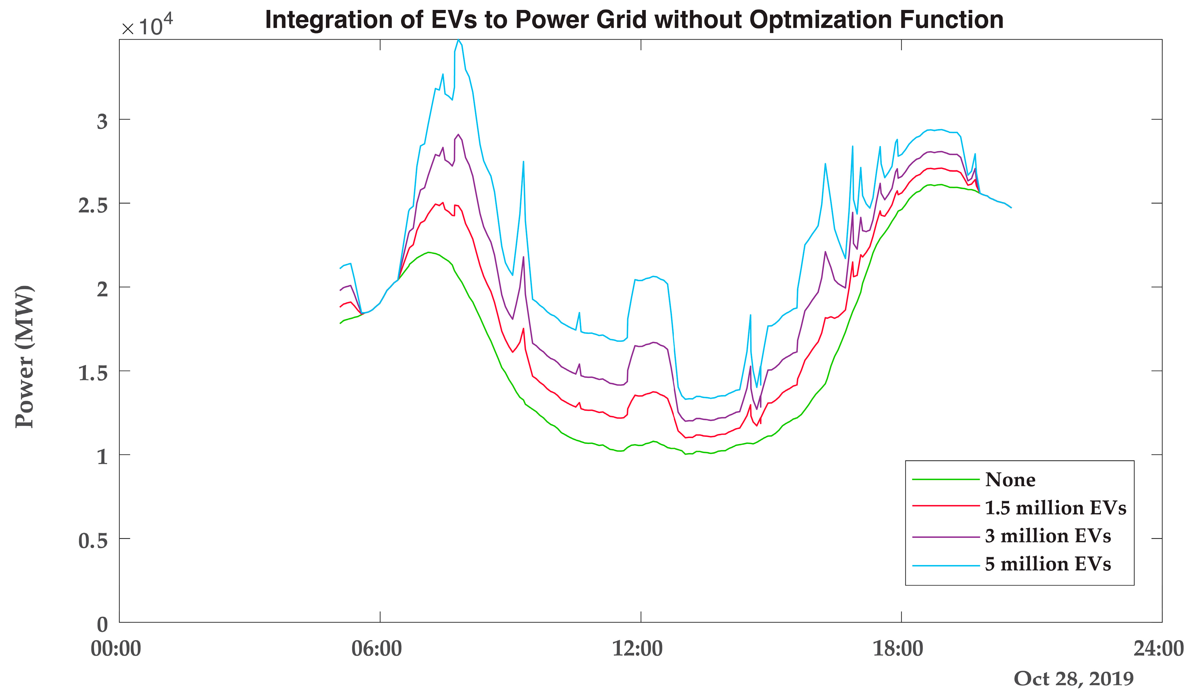
3.6. Impacts of EV Integration on Electric Power Grid

The state of California in the United States has set a goal for 100% zero-emission vehicle (ZEV) new-car sales by 2035. It is anticipated that around 5 million EVs will be on the road by 2030, with a target of 1.5 million EVs by 2025. A comparison of various scenarios—1.5 million, 3 million, and 5 million EVs integrated into the power grid—reveals that such integrations lead to increased fluctuations in grid stability, as illustrated in Figure 11. The figure was generated using the net power demands recorded on 28 October 2019.
Figure 12 and Figure 13 demonstrate that, with the proposed AI-driven charging strategies with U2 and U4 objective functions, grid fluctuations (such as those seen in the “duck curve”) are reduced, while charging is completed in a desirable charging duration with 1.5, 3, and 5 million EVs. Compared to the duck curves in Figure 10, the proposed charging strategies can reduce the peak power demand for smooth duck curves, suggesting the effectiveness of the proposed charging strategies. The peak power consumption reaches around 22,000 MW without EVs, 25,000 MW for 1.5 million EVs, 28,000 MW for 3 million EVs, and 35,000 MW for 5 million EVs without any charging strategy. By implementing an AI-driven optimal charging optimization strategy that considers both early charging and duck curve smoothing, the peak demand is reduced by approximately 16% for 1.5 million EVs, 21.43% for 3 million EVs, and 34.29% for 5 million EVs.
Figure 14 showed the duck curves with the integration of 10% of 1.5 million EVs into the system. Due to lesser EVs being integrated, the impact on charging power demands caused by EV charging requests is limited. The charging strategies with U2 and U4 objective functions still show a better performance as compared to the case with a non-optimal charging strategy.

4. Conclusions

Electric vehicles (EVs) are key solutions in intelligent transportation systems, due to their efficiency and reduced emissions. The efficient scheduling of EV charging is crucial for optimizing performance and grid stability. This research presents an AI-integrated optimal charging strategy aimed at enabling early charging and smoothing the power grid’s duck curve. Data from Caltech’s Adaptive Charging Network (ACN) at NASA’s Jet Propulsion Laboratory (JPL) were collected and divided into day and night charging patterns to predict the charging duration based on key input features, as follows: start charging time and energy requested. The predicted charging duration was then incorporated into optimization objective functions to enhance charging efficiency. Furthermore, the impacts of integrating 1.5 million, 3 million, and 5 million EVs were analyzed to assess system performance under the different levels of EV adoption. The proposed AI-based charging strategies integrated four different objective functions for optimization and showed the effectiveness of the charging strategies with various levels of EV adoption.
It is worth mentioning that discrepancies in the grid demand forecasts and variations in EV usage rates might pose significant challenges for real-world implementation. Since inconsistencies in demand forecasting models can impact the performance of AI-based charging strategies, the sensitivity of these results largely depends on forecasting accuracy. Unexpected grid disturbances, seasonal fluctuations in consumer demand, or sudden increases in EV usage may cause deviations from the optimal charging schedules. In addition, the proposed strategies can be enhanced by incorporating more factors such as adaptive pricing and incentives to promote off-peak charging, and battery energy storage systems can help manage high loads. In addition, the current research focuses on level 2 charging infrastructure, which is widely used for workplace and residential charging. Future work will extend this approach to DC fast charging, enabling real-time optimization for high-power charging stations. To prevent extreme peaks in the grid load while extending the study to DC fast charging infrastructure, the optimization approach would need to incorporate strategies such as load shifting, dynamic charging rates, the prioritization of charging schedules, energy storage, and advanced multi-objective optimization techniques. These adjustments can ensure that the high power demand associated with DC fast charging is managed effectively while maintaining grid stability. Furthermore, integrating state of health (SOH) estimation into the optimal charging strategy framework can improve the accuracy of cost evaluations in vehicle-to-grid systems.

Author Contributions

Conceptualization, U.J., R.J.A., S.A. and Y.-F.J.; methodology, U.J., S.A. and Y.-F.J.; software, U.J. and R.J.A.; validation, U.J. and R.J.A.; formal analysis, U.J.; investigation, U.J. and Y.-F.J.; resources, S.A. and Y.-F.J.; data curation, U.J. and R.J.A.; writing—original draft preparation, U.J.; writing—review and editing, S.A. and Y.-F.J.; supervision, Y.-F.J.; project administration, Y.-F.J.; funding acquisition, S.A. and Y.-F.J. All authors have read and agreed to the published version of the manuscript.

Funding

The authors acknowledge financial support for this research, authorship, and/or publication from the U.S. National Science Foundation (#2051113) and the U.S. Department of Transportation through the Transportation Consortium of South-Central States (Tran-SET) under projects 21034 and 21049.

Data Availability Statement

The original contributions presented in this study are included in the article. Further inquiries can be directed to the corresponding author.

Conflicts of Interest

The authors declare no conflicts of interest.

References

  1. U.S. Energy Information Administration. Use of Energy Explained. Available online: https://www.eia.gov/energyexplained/use-of-energy/transportation-in-depth.php (accessed on 12 January 2025).
  2. Mohanty, S.; Panda, S.; Parida, S.M.; Rout, P.K.; Sahu, B.K.; Bajaj, M.; Zawbaa, H.M.; Kumar, N.M.; Kamel, S. Demand side management of electric vehicles in smart grids: A survey on strategies, challenges, modeling, and optimization. Energy Rep. 2022, 8, 12466–12490. [Google Scholar]
  3. Das, H.S.; Rahman, M.M.; Li, S.; Tan, C. Electric vehicles standards, charging infrastructure, and impact on grid integration: A technological review. Renew. Sustain. Energy Rev. 2020, 120, 109618. [Google Scholar] [CrossRef]
  4. Rajper, S.Z.; Albrecht, J. Prospects of electric vehicles in the developing countries: A literature review. Sustainability 2020, 12, 1906. [Google Scholar] [CrossRef]
  5. Rapson, D.S.; Muehlegger, E. The economics of electric vehicles. Rev. Environ. Econ. Policy 2023, 17, 274–294. [Google Scholar] [CrossRef]
  6. Ahmad, A.; Khalid, M.; Ullah, Z.; Ahmad, N.; Aljaidi, M.; Malik, F.A.; Manzoor, U. Electric vehicle charging modes, technologies and applications of smart charging. Energies 2022, 15, 9471. [Google Scholar] [CrossRef]
  7. Tie, S.F.; Tan, C.W. A review of energy sources and energy management system in electric vehicles. Renew. Sustain. Energy Rev. 2013, 20, 82–102. [Google Scholar]
  8. Hussain, M.T.; Sulaiman, N.B.; Hussain, M.S.; Jabir, M. Optimal Management strategies to solve issues of grid having Electric Vehicles (EV): A review. J. Energy Storage 2021, 33, 102114. [Google Scholar]
  9. Elghanam, E.; Abdelfatah, A.; Hassan, M.S.; OSMAN, A. Optimization techniques in electric vehicle charging scheduling, routing and spatio-temporal demand coordination: A systematic review. IEEE Open J. Veh. Technol. 2024, 5, 1294–1313. [Google Scholar]
  10. Zhao, Y.; Guo, Y.; Guo, Q.; Zhang, H.; Sun, H. Deployment of the electric vehicle charging station considering existing competitors. IEEE Trans. Smart Grid 2020, 11, 4236–4248. [Google Scholar]
  11. Xiong, Y.; An, B.; Kraus, S. Electric vehicle charging strategy study and the application on charging station placement. Auton. Agents Multi-Agent Syst. 2021, 35, 1–19. [Google Scholar]
  12. Moghaddam, Z.; Ahmad, I.; Habibi, D.; Phung, Q.V. Smart charging strategy for electric vehicle charging stations. IEEE Trans. Transp. Electrif. 2017, 4, 76–88. [Google Scholar] [CrossRef]
  13. Hanemann, P.; Behnert, M.; Bruckner, T. Effects of electric vehicle charging strategies on the German power system. Appl. Energy 2017, 203, 608–622. [Google Scholar] [CrossRef]
  14. Soliman, I.A.; Tulsky, V.; Abd el-Ghany, H.A.; ElGebaly, A.E. Efficient allocation of capacitors and vehicle-to-grid integration with electric vehicle charging stations in radial distribution networks. Appl. Energy 2025, 377, 124745. [Google Scholar] [CrossRef]
  15. Ramkumar, A.; Rajesh, K. A design analysis of EV charging using multiport converter and control strategy using MWOA. J. Energy Storage 2025, 106, 114735. [Google Scholar]
  16. Lepolesa, L.J.; Adetunji, K.E.; Ouahada, K.; Liu, Z.; Cheng, L. Optimal EV Charging Strategy for Distribution Networks Load Balancing in a Smart Grid Using Dynamic Charging Price. IEEE Access 2024, 12, 47421–47432. [Google Scholar] [CrossRef]
  17. Khan, M.R.; Haider, Z.M.; Malik, F.H.; Almasoudi, F.M.; Alatawi, K.S.S.; Bhutta, M.S. A comprehensive review of microgrid energy management strategies considering electric vehicles, energy storage systems, and AI techniques. Processes 2024, 12, 270. [Google Scholar] [CrossRef]
  18. Yadav, K.; Singh, M. A novel energy management of public charging stations using attention-based deep learning model. Electr. Power Syst. Res. 2025, 238, 111090. [Google Scholar] [CrossRef]
  19. Arévalo, P.; Ochoa-Correa, D.; Villa-Ávila, E. A systematic review on the integration of artificial intelligence into energy management systems for electric vehicles: Recent advances and future perspectives. World Electr. Veh. J. 2024, 15, 364. [Google Scholar] [CrossRef]
  20. Recalde, A.; Cajo, R.; Velasquez, W.; Alvarez-Alvarado, M.S. Machine Learning and Optimization in Energy Management Systems for Plug-In Hybrid Electric Vehicles: A Comprehensive Review. Energies 2024, 17, 3059. [Google Scholar] [CrossRef]
  21. Alansari, M.; Al-Sumaiti, A.S.; Abughali, A. Optimal placement of electric vehicle charging infrastructures utilizing deep learning. IET Intell. Transp. Syst. 2024, 18, 1529–1544. [Google Scholar] [CrossRef]
  22. Shern, S.J.; Sarker, M.T.; Ramasamy, G.; Thiagarajah, S.P.; Al Farid, F.; Suganthi, S. Artificial Intelligence-Based Electric Vehicle Smart Charging System in Malaysia. World Electr. Veh. J. 2024, 15, 440. [Google Scholar] [CrossRef]
  23. Cavus, M.; Dissanayake, D.; Bell, M. Next Generation of Electric Vehicles: AI-Driven Approaches for Predictive Maintenance and Battery Management. Energies 2025, 18, 1041. [Google Scholar] [CrossRef]
  24. Khan, M.A.; Saleh, A.M.; Waseem, M.; Sajjad, I.A. Artificial intelligence enabled demand response: Prospects and challenges in smart grid environment. Ieee Access 2022, 11, 1477–1505. [Google Scholar]
  25. Lin, J.; Qiu, J.; Liu, G.; Yao, Z.; Yuan, Z.; Lu, X. A Fuzzy Logic Approach to Power System Security with Non-Ideal Electric Vehicle Battery Models in Vehicle-to-Grid Systems. IEEE Internet Things J. 2025. [Google Scholar] [CrossRef]
  26. Tian, X.; Zhou, S.; Hao, H.; Ruan, H.; Gaddam, R.R.; Dutta, R.C.; Zhu, T.; Wang, H.; Wu, B.; Brandon, N.P. Machine learning and density functional theory for catalyst and process design in hydrogen production. Chain 2024, 1, 150–166. [Google Scholar]
  27. Hassan, Q.; Azzawi, I.D.; Sameen, A.Z.; Salman, H.M. Hydrogen fuel cell vehicles: Opportunities and challenges. Sustainability 2023, 15, 11501. [Google Scholar] [CrossRef]
  28. Bree, G.; Hao, H.; Stoeva, Z.; Low, C.T.J. Monitoring state of charge and volume expansion in lithium-ion batteries: An approach using surface mounted thin-film graphene sensors. RSC Adv. 2023, 13, 7045–7054. [Google Scholar] [CrossRef]
  29. Dini, P.; Saponara, S.; Colicelli, A. Overview on battery charging systems for electric vehicles. Electronics 2023, 12, 4295. [Google Scholar] [CrossRef]
  30. Cadete, E.; Alva, R.; Zhang, A.; Ding, C.; Xie, M.; Ahmed, S.; Jin, Y. Deep learning tackles temporal predictions on charging loads of electric vehicles. In Proceedings of the 2022 IEEE Energy Conversion Congress and Exposition (ECCE), Detroit, MI, USA, 9–13 October 2022; pp. 1–6. [Google Scholar]
  31. Siddiqui, J.; Ahmed, U.; Amin, A.; Alharbi, T.; Alharbi, A.; Aziz, I.; Khan, A.R.; Mahmood, A. Electric Vehicle charging station load forecasting with an integrated DeepBoost approach. Alex. Eng. J. 2025, 116, 331–341. [Google Scholar] [CrossRef]
  32. Shanmuganathan, J.; Victoire, A.A.; Balraj, G.; Victoire, A. Deep learning LSTM recurrent neural network model for prediction of electric vehicle charging demand. Sustainability 2022, 14, 10207. [Google Scholar] [CrossRef]
  33. Almaghrebi, A.; Aljuheshi, F.; Rafaie, M.; James, K.; Alahmad, M. Data-driven charging demand prediction at public charging stations using supervised machine learning regression methods. Energies 2020, 13, 4231. [Google Scholar] [CrossRef]
  34. Li, C.; Dong, Z.; Chen, G.; Zhou, B.; Zhang, J.; Yu, X. Data-driven planning of electric vehicle charging infrastructure: A case study of Sydney, Australia. IEEE Trans. Smart Grid 2021, 12, 3289–3304. [Google Scholar] [CrossRef]
  35. Boulakhbar, M.; Farag, M.; Benabdelaziz, K.; Kousksou, T.; Zazi, M. A deep learning approach for prediction of electrical vehicle charging stations power demand in regulated electricity markets: The case of Morocco. Clean. Energy Syst. 2022, 3, 100039. [Google Scholar]
  36. Ran, J.; Gong, Y.; Hu, Y.; Cai, J. EV load forecasting using a refined CNN-LSTM-AM. Electr. Power Syst. Res. 2025, 238, 111091. [Google Scholar] [CrossRef]
  37. Straka, M.; De Falco, P.; Ferruzzi, G.; Proto, D.; Van Der Poel, G.; Khormali, S.; Buzna, L. Predicting popularity of electric vehicle charging infrastructure in urban context. IEEE Access 2020, 8, 11315–11327. [Google Scholar]
  38. Soldan, F.; Bionda, E.; Mauri, G.; Celaschi, S. Short-term forecast of electric vehicle charging stations occupancy using big data streaming analysis. In Proceedings of the 2021 IEEE International Conference on Environment and Electrical Engineering and 2021 IEEE Industrial and Commercial Power Systems Europe (EEEIC/I&CPS Europe), Bari, Italy, 7–10 September 2021; pp. 1–6. [Google Scholar]
  39. Mouaad, B.; Farag, M.; Kawtar, B.; Tarik, K.; Malika, Z. A deep learning approach for electric vehicle charging duration prediction at public charging stations: The case of Morocco. ITM Web Conf. 2022, 43, 01024. [Google Scholar]
  40. Ullah, I.; Liu, K.; Yamamoto, T.; Zahid, M.; Jamal, A. Prediction of electric vehicle charging duration time using ensemble machine learning algorithm and Shapley additive explanations. Int. J. Energy Res. 2022, 46, 15211–15230. [Google Scholar]
  41. Lu, X.; Qiu, J.; Lei, G.; Zhu, J. State of health estimation of lithium iron phosphate batteries based on degradation knowledge transfer learning. IEEE Trans. Transp. Electrif. 2023, 9, 4692–4703. [Google Scholar] [CrossRef]
  42. U.S. Department of Transportation. Charger Types and Speeds. Available online: https://www.transportation.gov/rural/ev/toolkit/ev-basics/charging-speeds (accessed on 23 October 2024).
Figure 1. Number of JPL sessions per day for Oct 2019. The number of days selected for model training is shown in the orange highlighted region.
Electronics 14 01471 g001
Figure 2. Structure of FFC-ANN with input, hidden, and output layers.
Electronics 14 01471 g002
Figure 3. Flow chart of the proposed AI-driven charging strategies.
Electronics 14 01471 g003
Figure 4. Correlation analysis among different data features.
Electronics 14 01471 g004
Figure 5. Data visualization for quality control (a) energy requested (b) start charging time, (c) charging duration of training data.
Electronics 14 01471 g005
Figure 6. Actual vs. FFC-ANN-predicted charging duration: (a) daytime pattern and (b) nighttime Pattern.
Electronics 14 01471 g006
Figure 7. FFC-ANN model validation: (a) daytime pattern and (b) nighttime pattern.
Electronics 14 01471 g007
Figure 8. Comparison between different AI Models: (a) daytime pattern and (b) nighttime pattern.
Electronics 14 01471 g008
Figure 9. California ISO power data in MW.
Electronics 14 01471 g009
Figure 10. Power (kW) by objective functions: U1: Linear charging schedule; U2: Duck curve smoothing; U3: Early/Quick Charging; U4: Early Charging + Duck curve smoothing for sessions at (a) Station ID AG-1F10 and (b) Station ID AG-4F38.
Electronics 14 01471 g010
Figure 11. Duck curves generated without adopting AI-driven strategy with 1.5 million, 3 million, and 5 million EVs.
Electronics 14 01471 g011
Figure 12. Duck curves generated by adopting AI-driven strategy using U2 objective function with 1.5 million, 3 million, and 5 million EVs.
Electronics 14 01471 g012
Figure 13. Duck curves generated by adopting AI-driven strategy using U4 objective function with 1.5 million, 3 million, and 5 million EVs.
Electronics 14 01471 g013
Figure 14. Duck curves generated for 10% of total of 1.5 million EVs with and without adopting AI-driven strategies.
Electronics 14 01471 g014
Table 1. Review of existing literature and contributions of proposed work.
ReferenceArtificial Intelligence
Technique
Optimal Charging
Strategy
EVs Impact on
Power Grid
[10,11]××
[12,13,14,15,16]×
[18,21,22,30,31,32,33,34,35,36,37,38,39,40]××
Proposed Work
Table 2. ACN charging sites for EVs.
Charging SiteLocationNo. of EVSENo. of EV Charging Sessions
2018201920202021Total
JPLA national research lab in
La Canada, California
52477517,4115576587633,638
CaltechResearch university in
Pasadena, California
5415,29710,6172472303831,424
Office 1An office building situated in the Silicon Valley area, California809224363251683
Table 3. Descriptions of EV charging data features. N/A stands for not applicable.
Data FeaturesDescriptionData TypeUnit
Connection TimeThe time when the EV is first plugged in and begins the charging session.datetimeN/A
Disconnect TimeThe time when the EV is unplugged, ending the charging session.datetimeN/A
Done Charging TimeThe time when the EV records its last instance of drawing a non-zero current, indicating that charging is complete.datetimeN/A
Energy RequestedThe amount of energy requested by the user for the charging session.floatkWh
Charging OccupancyThe total time an EV remains connected to a charging station(Difference between disconnect charging time and connection time).floath
Charging DurationThe total time taken for the EV to reach the requested charge level (Difference between done charging time and connection time).floath
PowerThe rate at which electrical energy is transferred to the EV battery during charging (Ratio between energy requested and charging duration).floatkW
Start Charging TimeThe connection time converted to hours after removing the date and zone information from timestamps.floath
Table 4. Factors for characterization of different models.
AI ModelLRGMRRFRFFC-ANN
TypeSimple
regression
Probabilistic model with mixture componentsEnsemble-based regressionNeural network
CharacteristicsLinear
relationship only, baseline models
Models complex, multimodal, and nonlinear
relationships
Nonlinear relationships via
ensemble trees
Models complex, nonlinear relationships
Handling
Nonlinearity
Cannot capture
nonlinearity without transformations
Captures multimodal and nonlinear relationshipsGood for complex, nonlinear relationshipsHighly capable of modeling
nonlinearity
Training
Complexity
LowModerate to high; EM algorithm can be intensiveMediumHigh, especially with deep architectures
ScalabilityHighModerate;
not as scalable for large datasets
Fairly high, but slows with more treesHigh computational demand
Table 5. Performance of FFC-ANN model at different hyperparameters for daytime pattern.
Sr. No.NeuronLearning RateLayerEpochsActivation FunctionBatch SizeMSEMAER2
1320.0013150tanh640.37330.42700.9066
2320.0013150tanh320.81710.65380.8788
3320.0013150tanh160.63280.60950.8732
4320.0013100tanh640.64100.59770.8732
5320.001350tanh640.74090.70820.7189
6320.013150tanh640.95830.74840.8444
7320.13150tanh640.92310.74390.8284
8640.0013150tanh640.64050.64270.8396
91280.0013150tanh640.66350.62830.8832
10320.0011150tanh641.55571.08300.6931
11320.0012150tanh640.76230.72500.8228
12320.0013150ReLU640.74940.61160.9010
13640.0013150ReLU640.33160.48860.9023
141280.0013150ReLU640.61670.63810.8759
15320.0013100ReLU640.66030.69520.8593
Table 6. Performance of FFC-ANN model at different hyperparameters for nighttime pattern.
Sr. No.NeuronLearning RateLayerEpochsActivation
Function
Batch SizeMSEMAER2
1320.0013150tanh640.16560.37230.9139
2320.0013150tanh320.17040.35820.9121
3320.0013150tanh160.16610.34590.9136
4320.0013100tanh640.19090.39910.9001
5320.001350tanh640.23920.41270.8133
6320.013150tanh640.18940.38290.9185
7320.13150tanh640.24570.37670.8162
8640.0013150tanh640.22380.43260.8871
91280.0013150tanh640.16000.35620.9159
10320.0011150tanh640.52410.57690.7168
11320.0012150tanh640.17120.36060.8778
12320.0013150ReLU640.12680.33400.9313
13640.0013150ReLU640.11630.31180.9355
141280.0013150ReLU640.10100.26650.9433
15320.0013100ReLU640.08730.25660.9214
Table 7. Performance of the FFC-ANN model at fixed hyperparameters.
Dataset Day   ( 6   a m T < 6   p m ) Night   ( 6   a m > T 6   p m )
Hyperparameter No.#12#13#12#13
Evaluation MetricsMSEMAER2MSEMAER2MSEMAER2MSEMAER2
Data Partitions10.74940.61160.90100.423 0.50370.9118 0.12680.33400.93130.10080.29130.9498
20.44590.51430.89920.33160.48860.90230.10070.27700.94770.08930.26210.9389
30.61000.61190.87930.56940.65250.89720.10920.29680.94280.10490.27690.9455
40.76400.66630.87330.40720.52060.91750.12780.33210.93960.10650.27680.9446
50.56650.60930.88000.53720.60340.90360.07660.24320.92680.16220.35780.9168
60.73520.71180.86250.59290.63770.89180.13780.33540.90540.11800.30930.9508
70.76190.71590.86290.47340.54900.89010.13320.34350.90740.13610.30240.9247
80.69650.69450.87520.46380.53820.89450.15510.34170.90700.09430.26380.9061
90.60810.65690.86220.66280.60930.88410.14550.32970.90160.06930.22020.9465
100.84620.79080.87790.53490.59870.89500.15900.30800.93320.13000.31510.9240
Mean0.67840.65830.87740.49970.57020.89880.12720.31410.92430.11110.28760.9348
Standard Deviation0.11890.07640.01390.09850.05750.01020.02550.03300.017370.02650.03710.0157
Table 8. Performance of FFC-ANN model for validation dataset.
Dataset Day   ( 6   a m T < 6   p m ) Night   ( 6   a m > T 6   p m )
Evaluation MetricsMSEMAER2MSEMAER2
Data Partitions10.53180.57190.87130.20000.37000.9352
20.78990.72510.87380.21220.40950.9155
30.45180.55400.86720.16720.35440.8978
40.56550.57660.89440.20420.40950.9250
50.56720.63730.88780.16480.35310.8908
60.78850.64010.86570.38250.36640.8975
70.41540.51540.91100.30190.43530.9044
80.77780.65460.86400.18790.36190.9057
90.63080.64320.86000.18670.33280.9122
100.63550.64030.92080.18970.37760.9276
Mean0.61540.61590.88160.21970.37710.9112
Standard Deviation0.13580.06080.02110.06890.03150.0146
Table 9. Performance of LR model.
Dataset Day   ( 6   a m T < 6   p m ) Night   ( 6   a m > T 6   p m )
Evaluation MetricsMSEMAER2MSEMAER2
Data Partitions10.77150.65050.87570.18860.38600.8554
20.99960.77450.84780.20590.41290.8418
31.17000.85860.80770.15270.36960.8625
41.00840.79060.80860.15270.35220.8883
50.82640.75270.85180.20320.40260.8722
60.90300.80010.81370.15480.34520.8903
70.61750.62450.85980.16250.35290.9092
80.82060.71990.86060.16410.37040.8974
90.86770.74580.81350.12760.31810.9353
101.19410.84940.80320.11280.29670.9112
Mean0.91790.75670.83420.16250.36070.8864
Standard Deviation0.16940.07250.02600.02860.03400.0272
Table 10. Performance of GMR model.
Dataset Day   ( 6   a m T < 6   p m ) Night   ( 6   a m > T 6   p m )
Evaluation MetricsMSEMAER2MSEMAER2
Data Partitions11.00340.81420.81140.27110.39790.8639
21.10240.91530.80860.33550.47880.8048
30.71350.68050.87050.34220.52820.8353
41.07610.73320.83320.21670.37400.8048
51.18960.75920.81360.30850.42680.8047
60.57840.62140.86950.37920.52110.8161
70.73030.70010.83950.40960.53670.8080
80.90890.79750.85160.23440.38060.8385
91.05570.82400.82750.23690.42140.8386
100.76360.67430.83710.20720.38790.8166
Mean0.91220.7520.83630.29410.44530.8231
Standard Deviation0.19360.08310.02120.06760.06150.0190
Table 11. Performance of RFR model.
Dataset Day   ( 6   a m T < 6   p m ) Night   ( 6   a m > T 6   p m )
Evaluation MetricsMSEMAER2MSEMAER2
Data Partitions10.59730.58470.87560.15590.34460.9193
20.62400.63390.89410.19270.37050.8921
30.82930.71370.86380.26270.45200.8857
40.49690.49970.88380.23960.40480.8789
50.59320.54280.87830.19090.34330.8805
60.67260.63200.83630.15290.28770.9303
70.98860.77180.83360.23480.38970.8654
80.78700.60850.86240.18200.34610.8999
90.92380.69110.82790.21500.36650.8812
100.81050.67120.87110.18870.30210.8689
Mean0.73230.63490.86270.20150.36070.8902
Standard Deviation0.15140.07710.02160.03420.04560.0199
Disclaimer/Publisher’s Note: The statements, opinions and data contained in all publications are solely those of the individual author(s) and contributor(s) and not of MDPI and/or the editor(s). MDPI and/or the editor(s) disclaim responsibility for any injury to people or property resulting from any ideas, methods, instructions or products referred to in the content.

