
Research on Estimation Optimization of State of Charge of Lithium-Ion Batteries Based on Kalman Filter Algorithm

Abstract
:1. Introduction
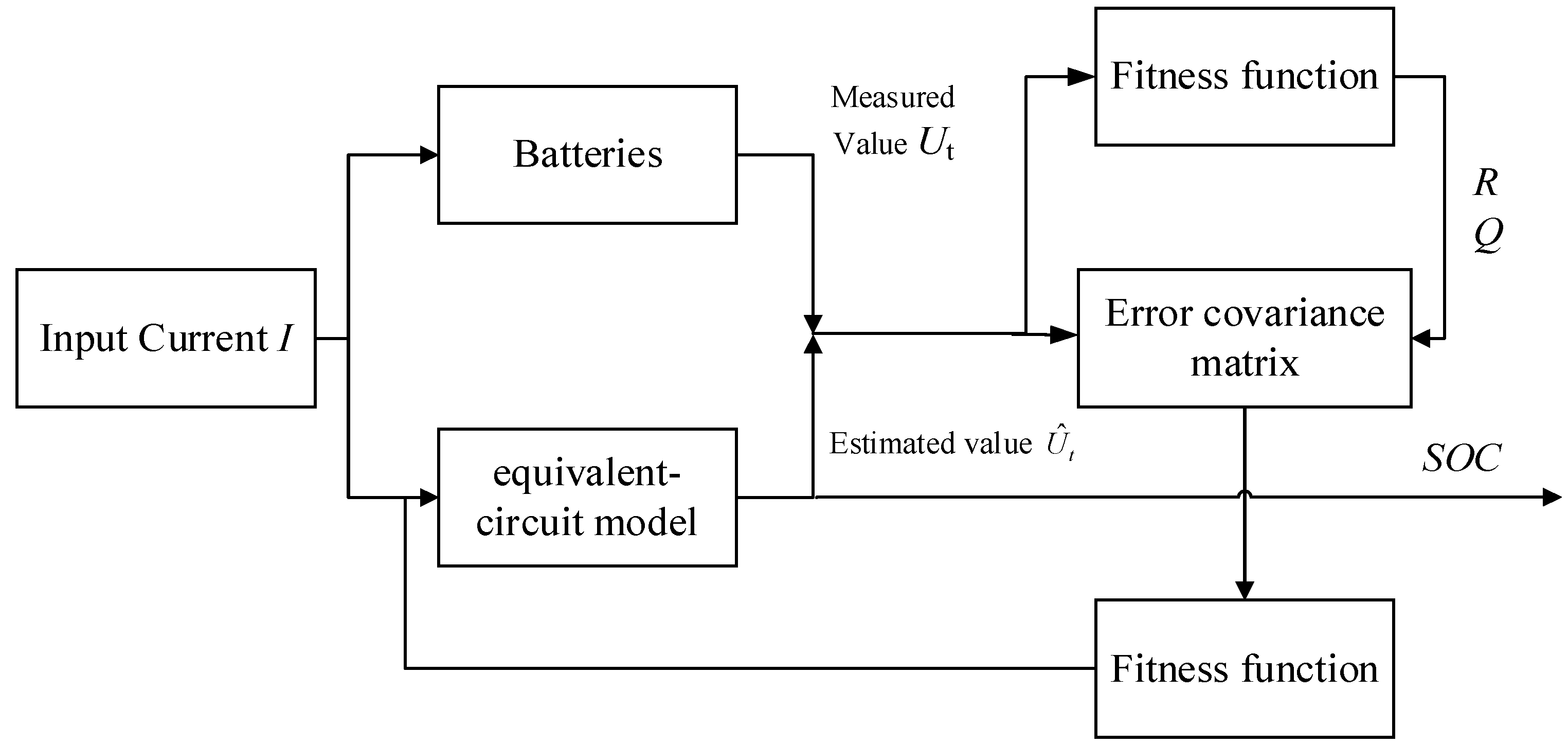
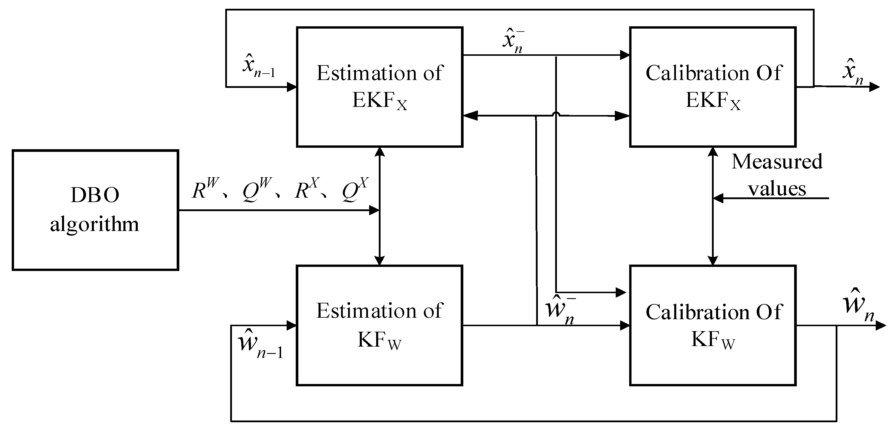
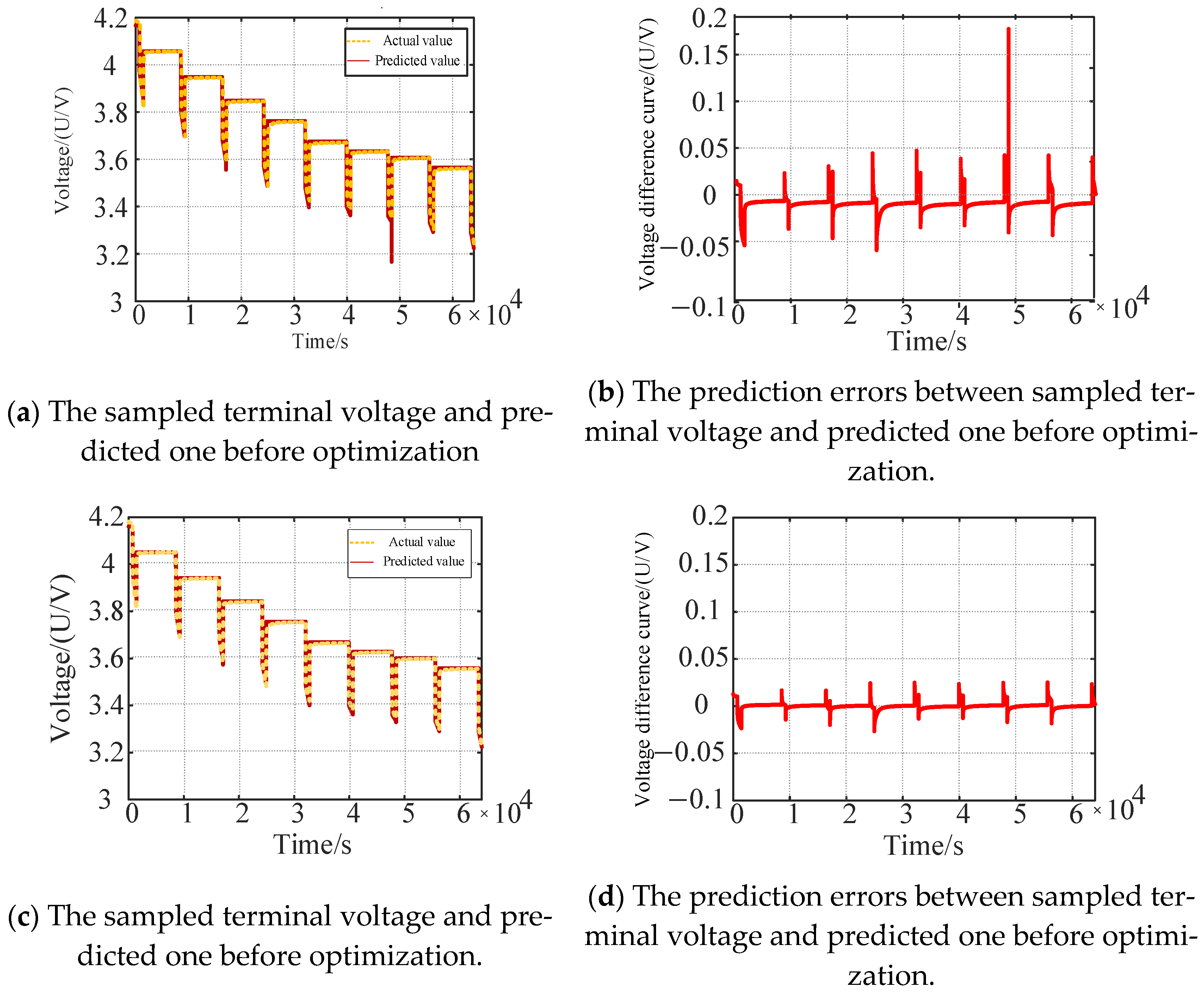
- This study designed the Dung Beetle Optimizer (DBO) secondary optimization Kalman filtering (DBO-DKF) algorithm as the SOC estimation method. The DBO algorithm targets the absolute accumulated error between the predicted terminal voltage of the power battery model under working conditions and the measured value. It optimizes the covariance matrices of system noise and observation noise in the iterative cycles of two Kalman filtering algorithms: one for model parameter identification (KF) and the other for SOC estimation (EKF).
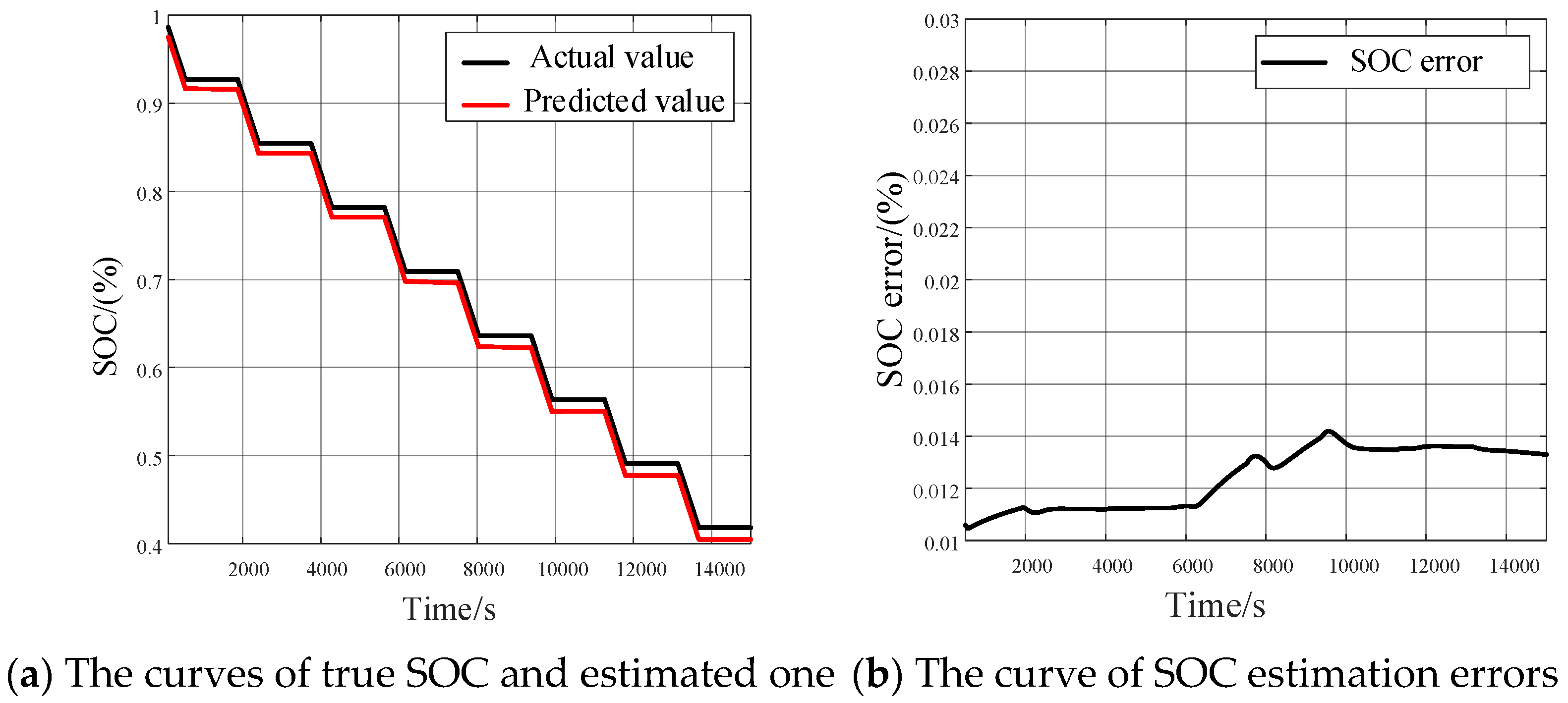
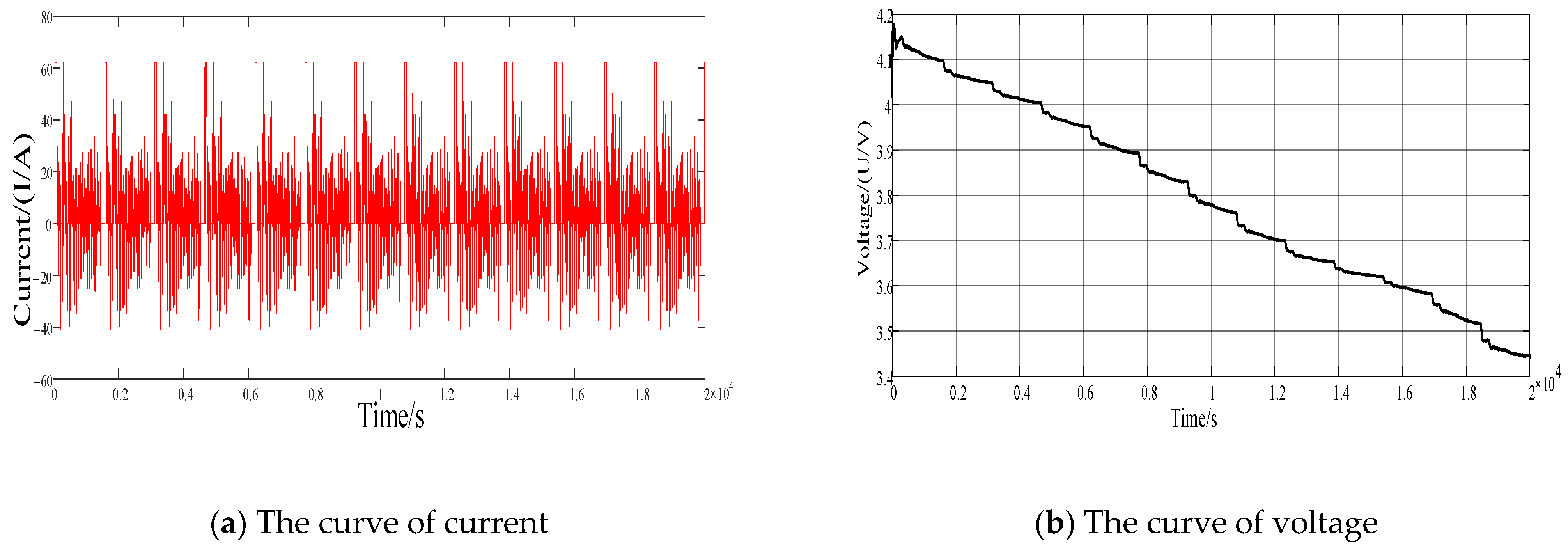
- This ensures real-time correction of the dynamic battery model and accuracy of experimental results. The study tested the DBO-DKF estimation method for power battery SOC under stable, complex, and realistic driving conditions of electric vehicles in the experimental phase. The optimization effects of the DBO-DKF algorithm in the parameter identification and SOC estimation stages were evaluated by comparing the sampled and estimated terminal voltage values, as well as the credibility indicators of SOC true values and estimated values.
- The research focused on the equivalent model parameter identification and SOC estimation of power batteries, utilizing the fast convergence speed and strong global search capability of the DBO algorithm. It addressed the issue of insufficient estimation accuracy caused by current and voltage measurement noise errors in the identification and estimation stages of the two Kalman filtering algorithms. The proposed DBO-DKF algorithm effectively enhances SOC estimation accuracy, computational efficiency, and robustness.
2. Materials and Methods
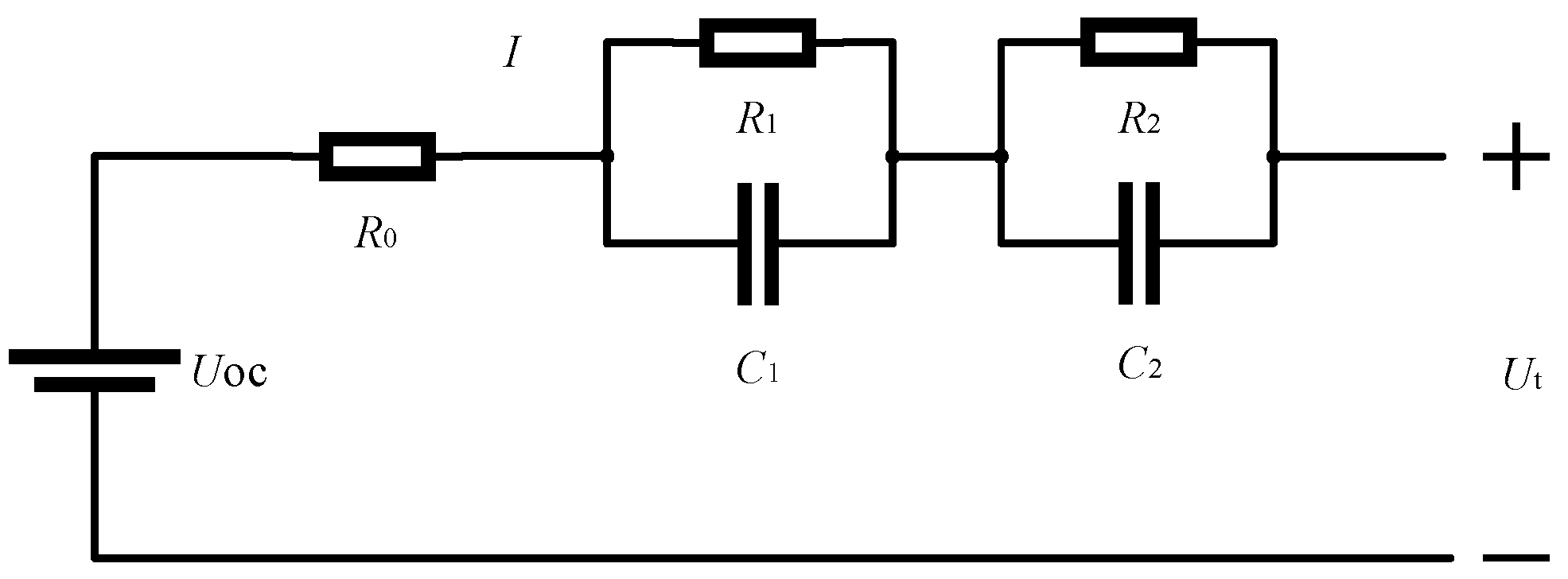
2.1. Creation of Lithium-Ion Battery Model
2.2. SOC Estimation with Kalman Filter Algorithm
2.2.1. Kalman Filter Algorithm
2.2.2. Principle of KF Algorithm for Estimating SOC
2.3. DBO Optimized Kalman Filter Algorithm
2.3.1. Dung Beetle Optimizer
- Position update mode of dung rolling beetles
- ①
- When there are no obstacles in the front:
- ②
- When there are obstacles in the front:
- 2.
- Position update mode of oviposition beetles
- 3.
- Position update mode of little beetles
- 4.
- Position update mode of thief beetles
2.3.2. Optimizing Kalman Filter Algorithm with Dung Beetle Optimizer
- Initialize parameters: Set the DBO population size (N), where each dung beetle corresponds to an initial set of parameters (q1,q2,r). These values are either randomly generated or empirically assigned within predefined boundaries.
- Define termination criteria: specify the maximum iteration count and convergence threshold to control the optimization process.
- Global search phase: Four categories of dung beetles perform randomized exploration in the parameter space to generate new solutions and identify the current best position. Calculate the fitness of each dung beetle’s position. The positional variables of the beetles act as independent variables in the fitness function, which are the elements in the covariance matrices Q (system noise) and R (measurement noise). After each iteration, compare the fitness of the updated positions of all dung beetles with the global best position. If the iteration count has not reached the predefined maximum, use the fitness values of the local best positions (individual beetles) and the global best position to determine whether convergence to the optimal solution has been achieved.
- Calculate the covariance matrix ∆ of the beetle’s position. If the matrix satisfies ∆ < ɛ (ɛ = 0.0001), it represents that the position of the t iteration is better, then update the beetle’s position variable to replace the original beetle’s position. Otherwise, keep the position unchanged until the loop position remains unchanged and the output position variable is the desired value. The absolute cumulative error between the predicted value CnXn,n−1 and measured value Zn of the terminal voltage is used as the algorithm fitness value (where L is the maximum sampling point):
- Output the optimal solution of the DBO-KF algorithm and assign it to the system noise covariance matrix R and Q.
2.3.3. SOC Estimation Based on DBO-DKF
3. Results
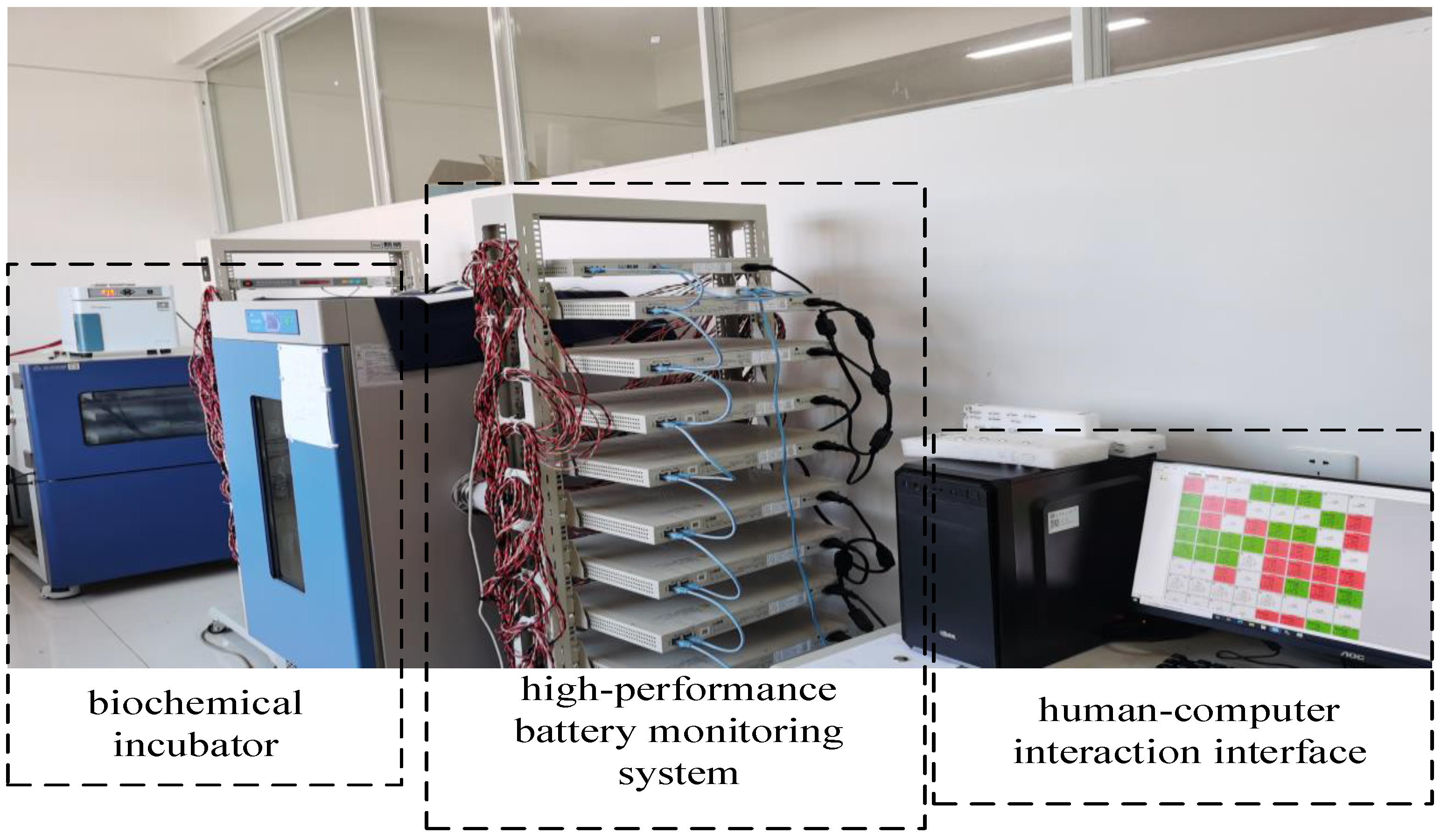
3.1. Establishment of the Experimental Platform
3.2. The SOC Optimization Under Various Practical Scenarios
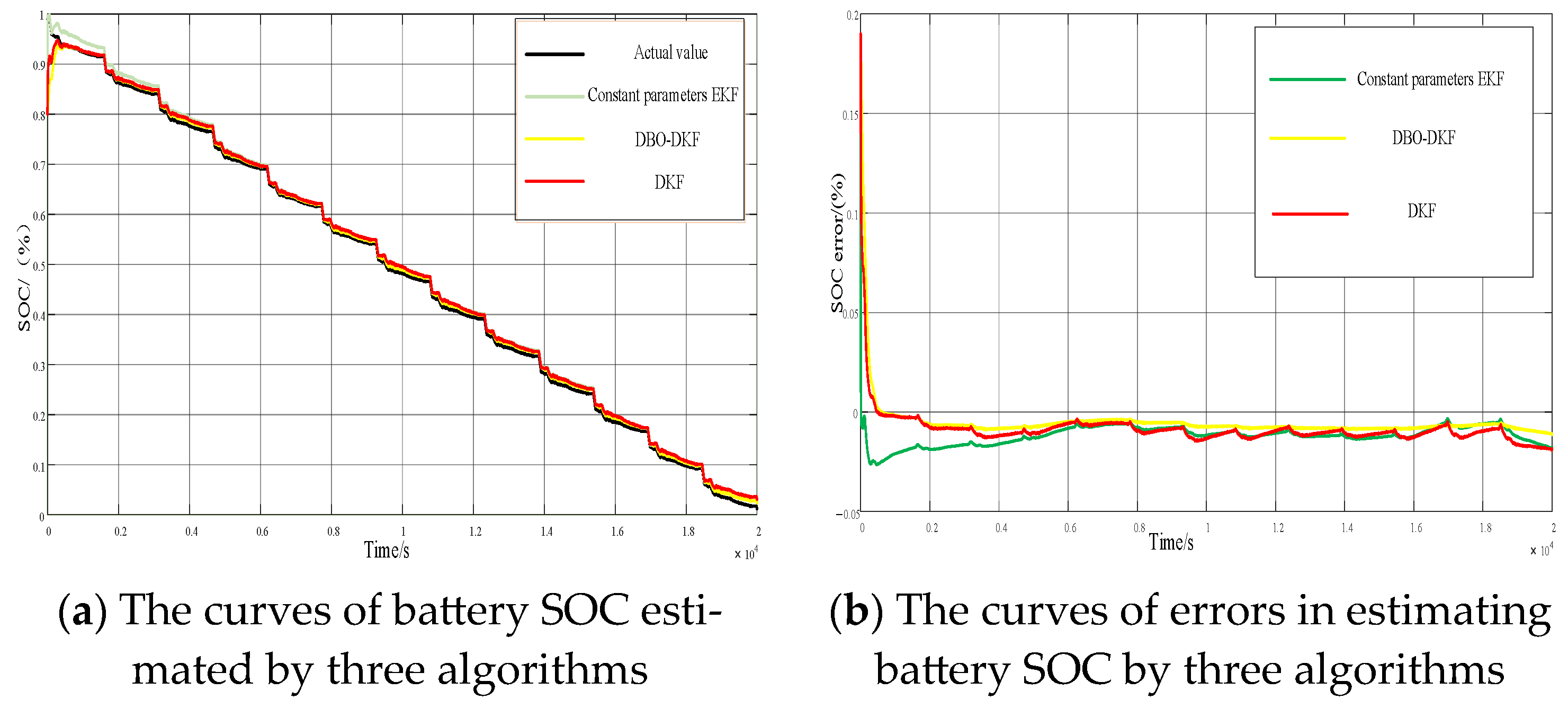
3.2.1. The Discharging Experiment of Battery Under Stable Condition
3.2.2. The Battery Discharging Experiment Under Complicated Scenarios
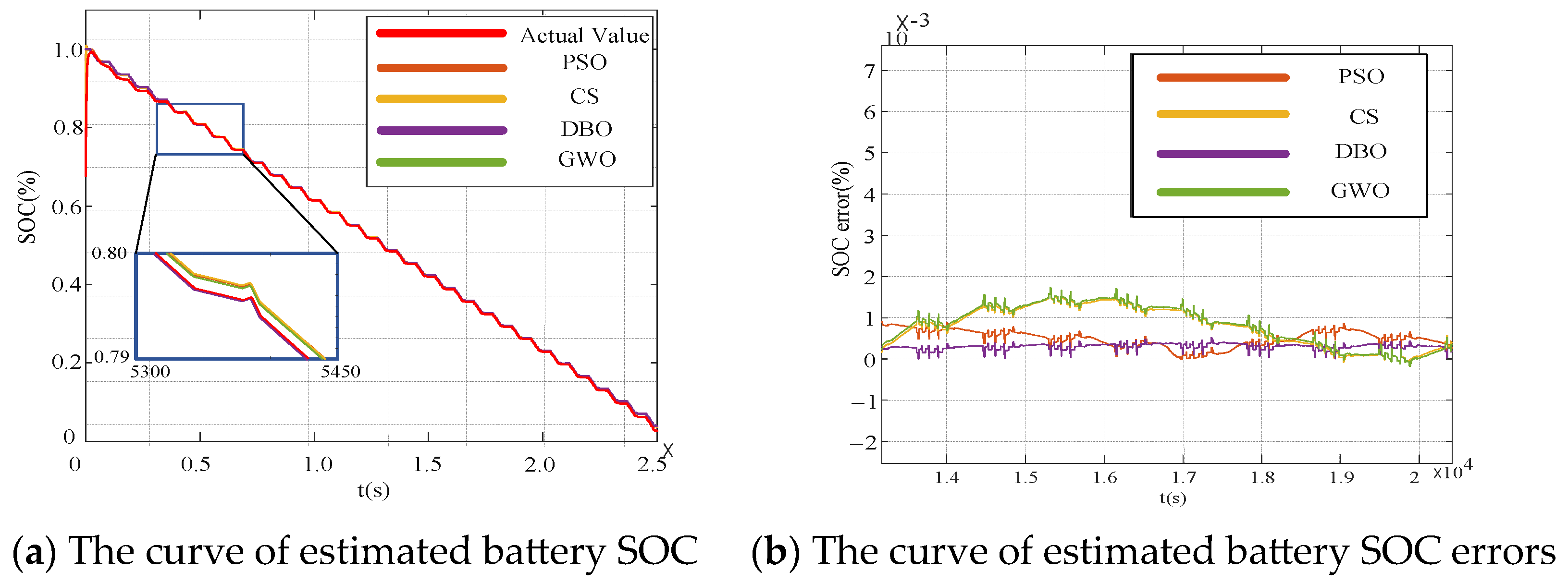
3.2.3. Comparison of Swarm Intelligence Algorithms for Optimizing the DKF Algorithm
3.2.4. The Battery SOC Estimation Based on DBO-DKF Algorithm Under Complicated Scenarios
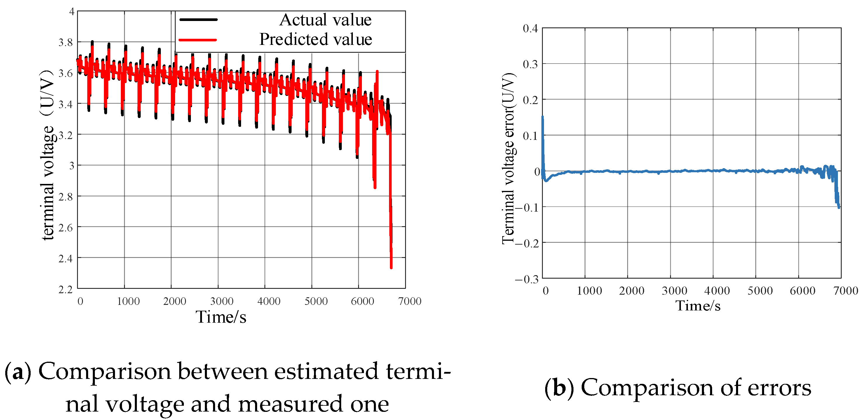
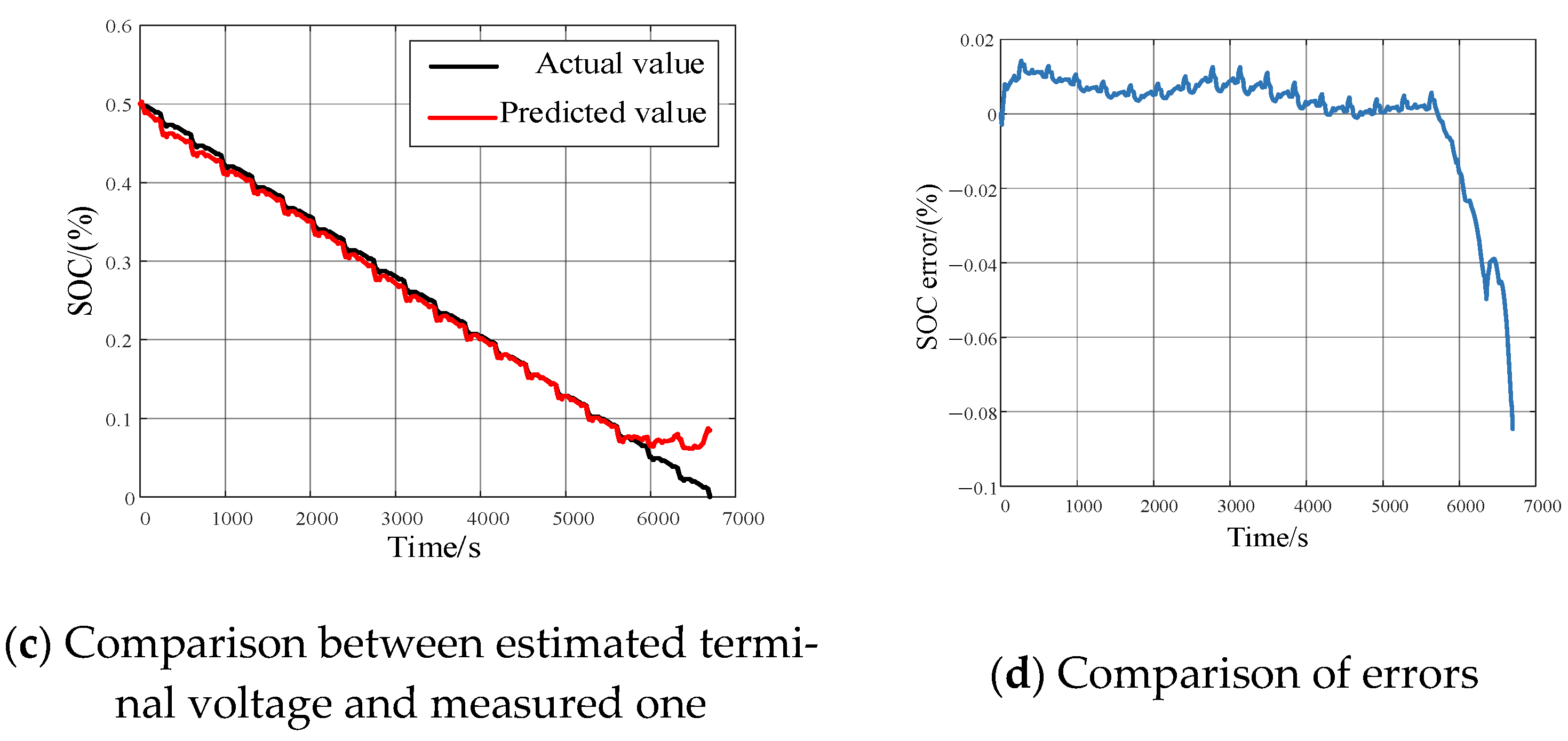
- The optimization performance under DST scenario
- The optimization performance under FUDS scenario
- The optimization performance under US60 scenario
- The optimization performance under BJDST scenario
4. Conclusions
Author Contributions
Funding
Data Availability Statement
Acknowledgments
Conflicts of Interest
References
- Bak, S.-M.; Nam, K.-W.; Chang, W.; Yu, X.; Hu, E.; Hwang, S.; Stach, E.A.; Kim, K.-B.; Chung, K.Y.; Yang, X.-Q. Correlating structural changes and gas evolution during the thermal decomposition of charged LixNi0.8Co0.15Al0.05O2 cathode materials. Chem. Mater. 2013, 25, 337–351. [Google Scholar]
- Fu, Y.; Zhai, B.; Shi, Z.; Liang, J.; Peng, Z. State of charge estimation of lithium-ion batteries based on an adaptive iterative extended Kalman filter for AUVs. Sensors 2022, 22, 9277. [Google Scholar] [CrossRef] [PubMed]
- Ma, T.; Xu, D.; Wei, M.; Wu, H.; He, X.; Zhang, Z.; Ma, D.; Liu, S.; Fan, B.; Lin, C.; et al. Study on lithium plating caused by inconsistent electrode decay rate during aging of traction batteries. Solid State Ion. 2020, 345, 115193. [Google Scholar]
- Xiang, S. Analysis of Potential Causes of Safety Failure of New Energy Vehicle Power Batteries. J. Electron. Res. Appl. 2023, 7, 13–19. [Google Scholar]
- Xie, Y.; Xu, J.; Jin, C.; Jia, Z.; Mei, X. A novel reduced-order electrochemical model of lithium-ion batteries with both high fidelity and real-time applicability. Energy 2024, 306, 132425. [Google Scholar]
- Nicodemo, N.; Di Rienzo, R.; Lagnoni, M.; Bertei, A.; Baronti, F. Estimation of lithium-ion battery electrochemical properties from equivalent circuit model parameters using machine learning. J. Energy Storage 2024, 99, 113257. [Google Scholar]
- Mele, I.; Zelič, K.; Firm, M.; Moškon, J.; Gaberšček, M.; Katrašnik, T. Enhanced Porous Electrode Theory Based Electrochemical Model for Higher Fidelity Modelling and Deciphering of the EIS Spectra. J. Electrochem. Soc. 2024, 171, 080537. [Google Scholar]
- Habte, B.T.; Jiang, F. Effect of microstructure morphology on Li-ion battery graphite anode performance: Electrochemical impedance spectroscopy modeling and analysis. Solid State Ion. 2018, 314, 81–91. [Google Scholar]
- Alavi, S.M.; Birkl, C.R.; Howey, D.A. Time-domain fitting of battery electrochemical impedance models. J. Power Sources 2015, 288, 345–352. [Google Scholar]
- Hu, J.N.; Hu, J.J.; Lin, H.B.; Li, X.P.; Jiang, C.L.; Qiu, X.H.; Li, W.S. State-of-charge estimation for battery management system using optimized support vector machine for regression. J. Power Sources 2014, 269, 682–693. [Google Scholar]
- Guo, X.; Xing, C.; Si, Y.; Zhu, J.; Xie, D. RLS adaptive equivalent circuit model of lithium battery under full working condition. Trans. China Electrotech. Soc. 2022, 37, 4029–4037. [Google Scholar]
- Chen, Z.; Yang, L.; Zhao, X.; Wang, Y.; He, Z. Online state of charge estimation of Li-ion battery based on an improved unscented Kalman filter approach. Appl. Math. Model. 2019, 70, 532–544. [Google Scholar] [CrossRef]
- He, L.; Wang, Y.; Wei, Y.; Wang, M.; Hu, X.; Shi, Q. An adaptive central difference Kalman filter approach for state of charge estimation by fractional order model of lithium-ion battery. Energy 2022, 244, 122627. [Google Scholar]
- Xia, B.; Huang, R.; Lao, Z.; Zhang, R.; Lai, Y.; Zheng, W.; Wang, H.; Wang, W.; Wang, M. Online parameter identification of lithium-ion batteries using a novel multiple forgetting factor recursive least square algorithm. Energies 2018, 11, 3180. [Google Scholar] [CrossRef]
- Gong, M.; Wu, J.; Jiao, C. SOC estimation method of lithium battery based on fuzzy adaptive extended Kalman filter. Trans. China Electrotech. Soc. 2020, 35, 3972–3978. [Google Scholar]
- Ma, W.; Guo, P.; Wang, X.; Zhang, Z.; Peng, S.; Chen, B. Robust state of charge estimation for Li-ion batteries based on cubature kalman filter with generalized maximum correntropy criterion. Energy 2022, 260, 125083. [Google Scholar]
- Cui, X.; Xu, B. State of charge estimation of lithium-ion battery using robust kernel fuzzy model and multi-innovation UKF algorithm under noise. IEEE Trans. Ind. Electron. 2021, 69, 11121–11131. [Google Scholar]
- Duan, L.; Zhang, X.; Jiang, Z.; Gong, Q.; Wang, Y.; Ao, X. State of charge estimation of lithium-ion batteries based on second-order adaptive extended Kalman filter with correspondence analysis. Energy 2023, 280, 128159. [Google Scholar]
- Sakile, R.; Sinha, U.K. Estimation of lithium-ion battery state of charge for electric vehicles using an adaptive joint algorithm. Adv. Theory Simul. 2022, 5, 2100397. [Google Scholar]
- He, H.; Xiong, R.; Zhang, X.; Sun, F.; Fan, J. State-of-charge estimation of the lithium-ion battery using an adaptive extended Kalman filter based on an improved Thevenin model. IEEE Trans. Veh. Technol. 2011, 60, 1461–1469. [Google Scholar]
- Pu, L.; Wang, C.; Chen, J. Lithium-ion batteries state of charge estimation using PSO-BP neural network improved UKF algorithm. In Proceedings of the 2024 39th Youth Academic Annual Conference of Chinese Association of Automation (YAC), Dalian, China, 7–9 June 2024; Volume 32, pp. 1988–1992. [Google Scholar]
- Zhang, X.; Hou, J.; Wang, Z.; Jiang, Y. Joint SOH-SOC estimation model for lithium-ion batteries based on GWO-BP neural network. Energies 2022, 16, 132. [Google Scholar] [CrossRef]
- Lyu, L.; Jiang, H.; Yang, F. Improved Dung Beetle Optimizer Algorithm with Multi-Strategy for global optimization and UAV 3D path planning. IEEE Access 2024, 12, 69240–69257. [Google Scholar] [CrossRef]
- Yang, J.; Zhang, Y.; Huang, Y.; Lv, J.; Wang, K. Multi-objective optimization of milling process: Exploring trade-off among energy consumption, time consumption and surface roughness. Int. J. Comput. Integr. Manuf. 2023, 36, 219–238. [Google Scholar] [CrossRef]
- Liu, J.; Lv, Z.; Zhao, L. A dual-optimization building energy prediction framework based on improved dung beetle algorithm, variational mode decomposition and deep learning. Energy Build. 2025, 328, 115143. [Google Scholar] [CrossRef]
- Xue, J.; Shen, B. Dung beetle optimizer: A new meta-heuristic algorithm for global optimization. J. Supercomput. 2023, 79, 7305–7336. [Google Scholar] [CrossRef]
- Qiu, X.; Wu, W.; Wang, S. Remaining useful life prediction of lithium-ion battery based on improved cuckoo search particle filter and a novel state of charge estimation method. J. Power Sources 2020, 450, 227700. [Google Scholar] [CrossRef]


| Number | Name | Dimension | Scope |
|---|---|---|---|
| F1 | Sphere | 30 | [100, 100] |
| F2 | Schwefel | 30 | [−10, 10] |
| F3 | Rastrigin | 30 | [5.12, 5.12] |
| F4 | Ackley | 30 | [−32, 32] |
| Function | Evaluation | DBO | CS | PSO | GWO |
|---|---|---|---|---|---|
| F1 | M Std | 2.02 × 10−104 1.11 × 10−103 | 4.95 × 10−97 2.48 × 10−96 | 1.17 × 10⁻⁵ 3.05 × 10⁻⁵ | 1.74 × 10⁻²⁷ 4.31 × 10⁻²⁷ |
| F2 | M Std | 1.37 × 10−80 7.48 × 10−79 | 7.91 × 10−66 4.33 × 10−65 | 77.11498 33.63623 | 8.39 × 10⁻⁶ 2.85 × 10⁻⁵ |
| F3 | M Std | 65.73226 26.76003 | 270.69723 397.69432 | 337.76123 685.57033 | 453.7054 732.1294 |
| F4 | M Std | 25.73226 0.19979 | 179.36765 143.84788 | 45.11843 26.76003 | 27.98438 0.415927 |
| Parameter | Value | Parameter | Value |
|---|---|---|---|
| Rated capacity | 2980 mA/h | Mass | 50.0 g |
| Rated voltage | 3.6 V | Charging temperature | +10~+45 °C |
| Maximum discharging current | 10 A | Discharging temperature | −20~+60 °C |
| Maximum charging current | 4 A | Charging–discharging cycles | 1000 |
| Energy density | 218 Wh/g | Size | 65.1 × 18.25 mm |
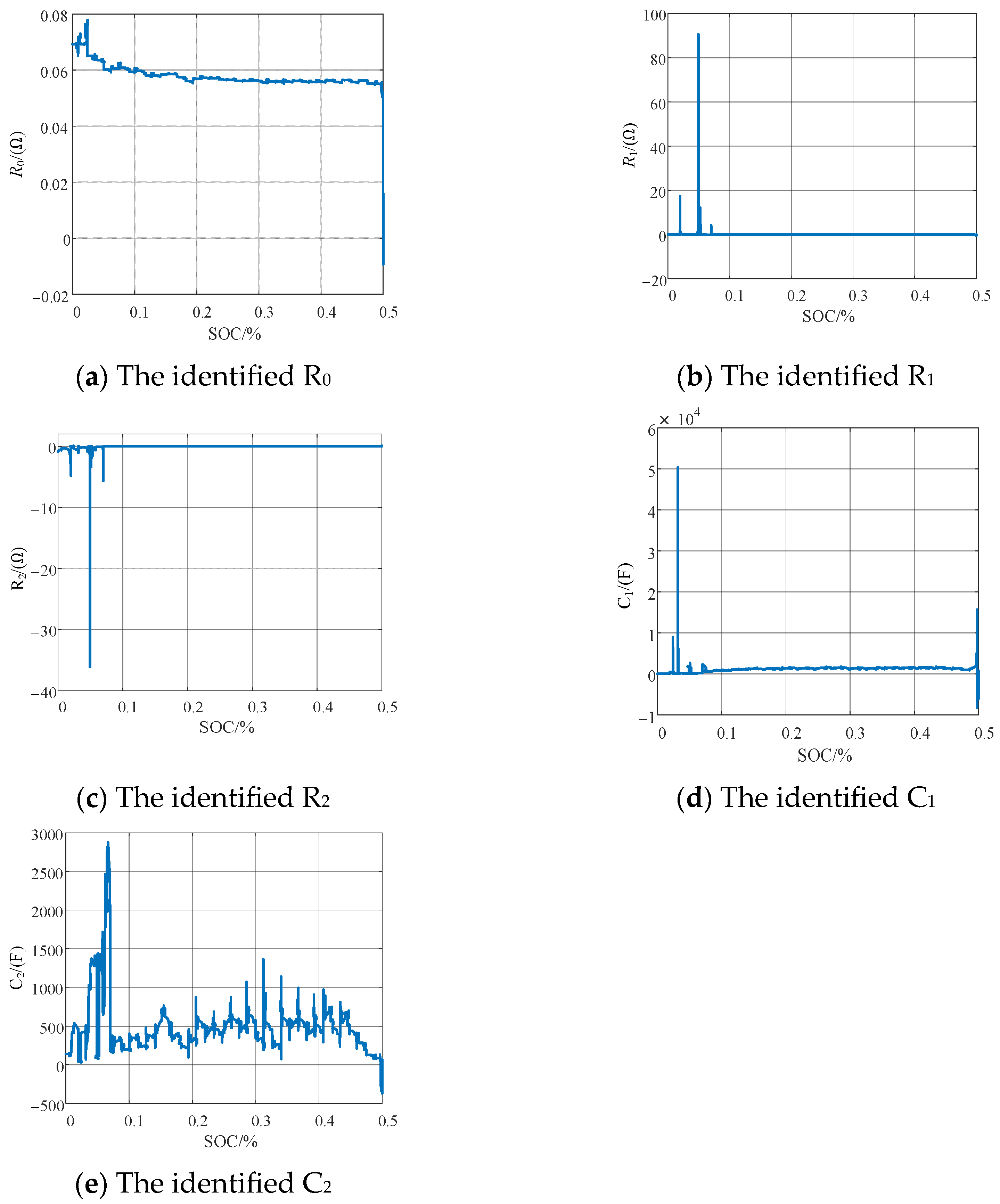
| SOC (%) | R0 (Ω) | R1 (Ω) | R2 (Ω) | C1 (F) | C2 (F) |
|---|---|---|---|---|---|
| 50% | 0.0090 | 0.1920 | 0.0943 | 9.8453 | 4.8505 |
| 40% | 0.0559 | 0.0394 | 0.036 | 151.2994 | 493.904 |
| 30% | 0.0561 | 0.0677 | 0.024 | 130.815 | 342.5928 |
| 20% | 0.0568 | 0.0568 | 0.0034 | 135.624 | 310.9536 |
| 10% | 0.0592 | 0.0286 | 0.0042 | 908.3162 | 191.9889 |
| 0% | 0.0692 | 0.0624 | −0.925 | 405.897 | 138.5594 |
| Parameter | Value |
|---|---|
| Internal resistance R0 | 0.0561 Ω |
| Polarization resistance R1 | 0.0677 Ω |
| Polarization capacitance C1 | 130.815 F |
| Polarization resistance R2 | 0.024 Ω |
| Polarization capacitance C2 | 342.5928 F |
| Errors | EKF | DKF | DBO-DKF |
|---|---|---|---|
| RMSE (%) | 6.0166 | 2.54736 | 1.7285 |
| MAE (%) | 3.8132 | 1.7389 | 1.7534 |
| R2 (%) | 0.88 | 0.91 | 0.95 |
| Errors | DBO | PSO | CS | GWO |
|---|---|---|---|---|
| RMSE | 0.043 | 0.048 | 0.058 | 0.092 |
| MAE | 0.032 | 0.036 | 0.045 | 0.068 |
| Index | DST | FUDS | US60 | BJDST |
|---|---|---|---|---|
| MSE (U/V) | 0.0299 | 0.00077 | 0.0012 | 0.017 |
| RMSE (U/V) | 0.000894 | 0.0278 | 0.0353 | 0.0408 |
| MAE (U/V) | 0.0134 | 0.0149 | 0.0163 | 0.0169 |
| Index | DST | FUDS | US60 | BJDST |
|---|---|---|---|---|
| MSE (%) | 2.23534 | 2.8138 | 2.23534 | 5.4309 |
| RMS (%) | 0.015 | 0.0167 | 0.01495 | 0.2925 |
| MAE (%) | 0.0092 | 0.0122 | 0.0092 | 0.2566 |
Disclaimer/Publisher’s Note: The statements, opinions and data contained in all publications are solely those of the individual author(s) and contributor(s) and not of MDPI and/or the editor(s). MDPI and/or the editor(s) disclaim responsibility for any injury to people or property resulting from any ideas, methods, instructions or products referred to in the content. |
© 2025 by the authors. Licensee MDPI, Basel, Switzerland. This article is an open access article distributed under the terms and conditions of the Creative Commons Attribution (CC BY) license (https://creativecommons.org/licenses/by/4.0/).
Share and Cite
Xia, T.; Xia, X.; Yue, J.; Gong, Y.; Tan, J.; Wen, L. Research on Estimation Optimization of State of Charge of Lithium-Ion Batteries Based on Kalman Filter Algorithm. Electronics 2025, 14, 1462. https://doi.org/10.3390/electronics14071462
Xia T, Xia X, Yue J, Gong Y, Tan J, Wen L. Research on Estimation Optimization of State of Charge of Lithium-Ion Batteries Based on Kalman Filter Algorithm. Electronics. 2025; 14(7):1462. https://doi.org/10.3390/electronics14071462
Chicago/Turabian StyleXia, Tian, Xiangyang Xia, Jiahui Yue, Yu Gong, Jianguo Tan, and Lixing Wen. 2025. "Research on Estimation Optimization of State of Charge of Lithium-Ion Batteries Based on Kalman Filter Algorithm" Electronics 14, no. 7: 1462. https://doi.org/10.3390/electronics14071462
APA StyleXia, T., Xia, X., Yue, J., Gong, Y., Tan, J., & Wen, L. (2025). Research on Estimation Optimization of State of Charge of Lithium-Ion Batteries Based on Kalman Filter Algorithm. Electronics, 14(7), 1462. https://doi.org/10.3390/electronics14071462