Leveraging Prototypical Prompt Learning for Robust Bridge Defect Classification in Civil Infrastructure

Abstract

Despite significant advancements in bridge façade defect classification, real-world automated inspections continue to face substantial challenges, including faint defect visibility, low lighting conditions, overexposure, noise interference, motion blur, and occlusions. These factors, stemming from variable environmental conditions and unstable imaging angles, severely degrade model performance. To address this issue, we introduce the Hard Defect Classification Dataset (HDCD), which systematically incorporates these six challenging conditions. Benchmarking state-of-the-art (SOTA) methods on the HDCD reveals a substantial performance drop on hard samples, highlighting the limitations of existing approaches in capturing class-specific features under adverse conditions. To enhance robustness, we propose the Prototypical Prompt Learning Framework (PPLF), inspired by prompt learning. PPLF utilizes category prototype vectors as dynamic prompts to interact with query features, guiding the model to focus on defect regions while suppressing background noise. A hierarchical feature fusion mechanism further integrates low-level texture details with high-level semantic patterns, improving defect localization and classification. Extensive experiments on ResNet-50, EfficientNetV2-L, and ViT demonstrate that PPLF consistently outperforms SOTA methods, especially achieving a 7% improvement on ResNet-50, showcasing its effectiveness in real-world civil engineering applications where robustness to challenging conditions is critical.

1. Introduction

As critical elements of modern infrastructures, bridges facilitate transportation and commerce across vast distances. However, like all infrastructures, bridges are susceptible to wear and tear, environmental degradation, and the inherent limitations of their materials and construction methods [1]. Given the critical role bridges play in daily life, it is essential for governments to detect defects early to prevent catastrophic failures. The cost of manual inspections and maintenance is substantial, with reports indicating that China’s bridge inspection and maintenance service market is one of the largest in the world, growing at rates higher than the global average.

Historically, bridge defect inspection relied heavily on manual checks, where engineers had to physically inspect various parts of the bridge using basic tools. This process was time-consuming, expensive, and limited by the inspectors’ experience and skills, making it difficult to identify potential internal defects. Furthermore, the frequency and coverage of manual inspections were restricted, preventing real-time monitoring of bridge health. With technological advancements, semi-automated equipment, such as ultrasonic detectors [2] and infrared thermography cameras [3], have been introduced to enhance the efficiency of defect categorization. Automatic defect classification in the civil engineering sector has become a significant task, which could reduce both the financial burden and the risk of accidents. But this method still required professional operation and manual data analysis, preventing full automation. In recent years, digital twin technology has emerged as a promising solution, enabling intelligent bridge health monitoring systems to collect real-time data on stress, displacement, temperature, and other factors through sensors installed on critical points [4]. While these systems offer valuable insights into bridge health, they still cannot distinguish defect categories well, especially some uncommon ones. Deep learning is essential for this task.

At the early stages, visual methods for concrete defect classification attempted to devise suitable features to characterize defects, both in the spatial and spectral domains [5,6]. Some of these methods were successful in classifying single defects such as cracks and rust [7], but their performance deteriorated dramatically when dealing with other types of defects. Then, some architectures, such as ResNet [8], EfficientNet [9], and InceptionV4 [10], revolutionized the ways of classifying images; Convolutional Neural Networks (CNNs) became the standard for computer vision. CNNs can extract unique features from images to create meaningful representations for image classification. Subsequently, some engineers integrated visual technologies into robotic platforms [11,12] that allow for timely detection of defects in remote areas and large bridge infrastructures, enhancing both efficiency and safety.

Despite these advancements, defect classification in the civil engineering field still faces a lot of challenges. One of the primary issues is the limited availability of labeled data for training, as the number of defect samples is far smaller than in conventional image datasets. And acquiring sufficient defect samples can be costly or even unfeasible, especially when defect categories have low incidence rates. Several researchers have proposed semi-supervised learning to address this shortage. For example, a generative adversarial network (GAN) [13] was developed to artificially generate many unlabeled samples, and a multi-training algorithm was used to integrate labeled and unlabeled samples into a semi-supervised learning process. Ref. [14] proposed a new approach that utilizes the semi-supervised generative adversarial network (SGAN) in YOLOv2 to facilitate the ability of the convolutional auto encoder (CAE) [15] to generate unique features. Note that these semi-supervised methods still require a large number of unlabeled defect images, which are often not available for industrial inspection tasks. To solve such few-shot problems, some people choose to pre-train a classifier on open source datasets (e.g., ImageNet [16] and CUB [17]) and then migrate the pre-trained parameters to classify bridge defects. But these typical datasets for few-shot learning mainly include semantic classes such as a bicycle, bird, and chair. In contrast, in façade defects, the difference between classes of defects is mainly texture information rather than semantic. Therefore, models trained on visual object datasets are not fully suitable for the classification of elevation defects.

Based on this, some studies have proposed using prompt learning to improve the classification of bridge images [18]. Although prompt learning has shown promising results in certain scenarios, Figure 1 shows that it still struggles with difficult samples typically encountered in real-world environments.

These samples often suffer from noise, dim lighting, and partial occlusion, making them significantly harder to classify compared to data collected under controlled conditions. This limitation stems from the fact that prompt-based methods are usually trained on curated or augmented datasets with clear and easily identifiable defect features. In real-world applications, however, for such as UAV-based inspections [19,20], images often exhibit inadequate lighting, complex backgrounds, and other challenging conditions. Traditional prompts and methods fail to sufficiently address these complexities, underscoring the need for new strategies to enhance classification in such environments.

In this study, we tackled the issue of poor model generalization in real-world applications where complex environments increase sample difficulty beyond that of the training data. To tackle this issue, we present the following contributions: (1) we constructed the Hard Defect Classification Dataset (HDCD), which simulates the complex conditions encountered in real-world scenarios. This dataset includes factors such as small targets, image blurring, noise, and other challenging conditions to provide a more realistic evaluation of a model’s performance. (2) To address the generalization challenges posed by real-world environmental factors such as noise, low lighting, and occlusion, we propose the Prototypical Prompt Learning Framework (PPLF), as illustrated in Figure 2. Our framework leverages interactions between category prototype features and the features of challenging real-world samples, enhancing a model’s ability to focus on defective targets while minimizing interference from background features. (3) Our experiments demonstrate that the proposed approach effectively adapts to complex scenes, significantly enhancing a model’s performance on challenging samples.

2. Related Work

2.1. Deep Learning for Bridge Defect Classification

Bridge defects can appear in diverse forms, ranging from microscopic material fatigue to macroscopic issues such as misalignment and compromised load-bearing capacity. These may include but are not limited to corrosion, cracks, deformation, scour, and inadequate maintenance practices. Each defect has the potential to escalate from a minor inconvenience to a catastrophic failure if not identified and addressed promptly.

In recent years, bridge defect classification technology based on deep learning methods has garnered widespread attention. Deep learning approaches can achieve superior performance compared to traditional machine learning methods, such as Support Vector Machines (SVMs) [21] and Random Forests [22], but at the cost of requiring abundant labeled data. Additionally, the impact of different color spaces, sliding window sizes, and CNN architectures has been discussed to achieve the most suitable configuration. The quality of the training data also plays a crucial role in determining the performance of deep learning models. Consequently, some previous studies have proposed methods to enhance classification accuracy by modifying a model’s adaptability to data. However, these methods largely rely on abundant training data and cannot be extended to the classification of unseen classes.

2.2. Prompt Learning in Image Classification

Prompts were initially introduced in natural language processing (NLP) as structured inputs designed to guide models in performing specific tasks [23,24]. In this context, prompts are first converted into vector representations, which are then processed through a multi-layer neural network, primarily leveraging a self-attention mechanisms [25]. The model assigns attentional weights to each token within the prompt to capture relationships and guide subsequent predictions, such as generating text or answering questions [26]. Prompt learning builds on this idea by designing or learning task-relevant prompts that reframe problems into formats more interpretable by pre-trained models [27]. This approach enables tasks to be performed with minimal or even no labeled data, making it an effective fine-tuning technique for pre-trained large language models (LLMs) [28] such as LLaMA [29] and GPT [30].

Recently, vision–language models (VLMs) like CLIP [31] and ALIGN [32] have bridged textual prompts with visual models, mapping images and text into a shared embedding space to facilitate generalizable visual representations. These can be applied to various downstream classification tasks using prompts. For instance, new classification weights can be synthesized by providing sentences describing relevant categories to a text encoder, which are then compared with image features generated by the image encoder. While textual prompts play a critical role in downstream tasks, crafting effective prompts can be challenging and time-consuming, as small variations in wording often lead to significant performance changes. To address this, advanced prompt engineering methods have introduced automatic adjustments based on contextual information to enhance performance [33].

Recognizing the inherent disparities in information density between visual and NLP tasks, researchers have adapted the concept of prompts for purely visual tasks. Visual prompts often involve introducing adaptive parameters that pre-populate model inputs or interact directly with target images as vector representations [34]. These visual prompts can be fine-tuned through gradient-based optimization [35], enhancing their utility in vision-specific tasks. Building upon this foundation, we extend the application of prompt learning to improve a model’s generalization on challenging samples, incorporating task-related information to address challenges in defect classification effectively.

3. Methodology

3.1. Problem Definition

In real-world bridge inspection scenarios, automated data collection often encounters significant challenges due to variable environmental conditions, unstable shooting angles, and complex working environments. These factors result in test samples that exhibit a range of challenging conditions. Which make it difficult for existing deep learning models to accurately classify defects, as they struggle to capture class-specific features under these adverse scenarios. To address these challenges, we define a clear problem setting for our study:

The training data ${\mathcal{D}}_{train}$ consist of high-quality bridge defect images captured under controlled, normal conditions. These images provide a balanced representation of defect categories, enabling the model to learn robust feature representations. The test data ${\mathcal{D}}_{test}$ comprise hard samples specifically curated to simulate real-world acquisition challenges. These samples are artificially modified to include conditions such as reduced brightness, added noise, and simulated occlusions, ensuring that the test set reflects the variability encountered in practical inspections. Importantly, the training and test sets are mutually exclusive ${\mathcal{D}}_{train}\cap {\mathcal{D}}_{test}=\varnothing$ to ensure an unbiased evaluation of the model’s generalization capabilities.

The core challenge lies in bridging the gap between the well-defined features learned from ${\mathcal{D}}_{train}$ and the complex, noisy patterns present in ${\mathcal{D}}_{test}$. Existing methods often fail to generalize to hard samples because they rely on static feature representations that are sensitive to environmental variations. To address this, we propose the Prototypical Prompt Learning Framework (PPLF), which leverages category prototype vectors to dynamically adapt a model’s feature space to challenging conditions. These prototypes, computed as the mean feature representations of each category in ${\mathcal{D}}_{train}$ [36], serve as robust anchors that guide the model to focus on defect-specific patterns while minimizing the impact of background noise. These vectors are defined as follows: given K categories, each with a feature set $\{x_i^c\mid i=1,\dots ,M_c,c=1,\dots ,K\}$, where $x_i^c$ is the feature vector for the i-th sample in category c, $M_c$ is the number of samples in category c. And the prototype feature vector $P_c$ is computed as a class mean:

$$\begin{array}{c}\hfill P_c={\displaystyle \frac{1}{M_c}}\sum _{i=1}^{M_c}{x}_i^c\end{array}$$

(1)

Given an input query image ${\mathbf{x}}_q\in {\mathbb{R}}^{C\times H\times W}$ from the test set ${\mathcal{D}}_{\mathrm{test}}$, where H, W, and C denote the height, width, and channel dimensions of the image, respectively, the task is to classify ${\mathbf{x}}_q$ into one of K predefined defect categories, denoted as $y_q\in \{1,2,\dots ,K\}$. To achieve this, we leverage class prototype features $P_c\in {\mathbb{R}}^d$, where $c\in \{1,2,\dots ,K\}$, which are computed as the mean feature representations of each category from the training set ${\mathcal{D}}_{\mathrm{train}}$.

The classification task is then formulated as a nearest-prototype assignment problem in the feature space. Specifically, the query image ${\mathbf{x}}_q$ is assigned to the category whose prototype $P_c$ is most compatible with its feature representation $f_{\theta }\left({\mathbf{x}}_q\right)$. This compatibility is quantified using a learned metric function $g_{\varphi }(·,·)$, which measures the similarity between the query feature and each prototype:

$$\begin{array}{c}\hfill y_q=arg\underset{c\in \{1,2,\dots ,K\}}{max}{g}_{\varphi }(f_{\theta }\left({\mathbf{x}}_q\right),P_c).\end{array}$$

(2)

Here, $g_{\varphi }(·,·)$ is implemented as a multi-layer neural network that learns task-specific similarity metrics, enabling the model to adaptively weigh feature dimensions based on their discriminative power. This formulation not only improves classification accuracy but also enhances interpretability, as the prototypes provide a clear representation of each defect category’s characteristic features. By leveraging prototype-based feature alignment, our framework addresses the challenges posed by hard samples in ${\mathcal{D}}_{\mathrm{test}}$, ensuring robust performance in real-world bridge inspection scenarios where environmental variability and complex conditions are prevalent.

3.2. Overview

Unlike semantic image classes with distinct overall contours, bridge defects are primarily characterized by subtle texture-level features. These defects often lack clear outlines and are easily confused with normal elements on the concrete surface, such as horizontal lines, graffiti, or other surface irregularities; see Figure 3 for details. This blending of defect features with background noise poses significant challenges for accurate classification, especially in real operating environments.

To address the need for the fine-grained processing of real-world bridge images with common quality issues like blurring, occlusion, and poor lighting, we propose the Prototypical Prompt Learning Framework (PPLF). This approach significantly improves a model’s ability to identify defect targets under challenging imaging conditions. By utilizing class prototype $P_c$ as prompts, PPLF facilitates the Category-Enhanced Representation Module (CERM) and Feature Fusion Classifier (FFC) to effectively capture fine-grained relationships between query images and class prototypes, thereby improving classification performance. First, we apply the randaugment [37] method to the origin query image $\mathbf{I}\in {\mathbb{R}}^{H\times W\times C}$. It has a data augment operations collection $\mathcal{T}=\{T_1,T_2,\dots ,T_K\}$, where each $T_k$ is an operation like rotate, flip, and crop. Then, randaugment randomly selects N operations from $\mathcal{T}$ that transform the original image $\mathbf{I}$ with magnitude M. The formula is shown below:

$$\begin{array}{c}\hfill {\mathbf{I}}^{\prime }=\left(\prod _{j=1}^N{T}_{i_j}(·,M)\right)\left(\mathbf{I}\right)\end{array}$$

(3)

where ∏ denotes a combination of operations. Subsequently, the backbone extracts ${\mathbf{I}}^{\prime }$ as image features ${\mathbf{x}}_q\in {\mathbb{R}}^{H\times W\times C}$ along with a prototype feature set $\mathbf{P}=\{P_c\mid c=1,\dots ,K\}\in {\mathbb{R}}^{K\times C\times H\times W}$ into the CERM. The prototype vectors are utilized to enhance the query representation, producing an enhanced query feature ${\mathbf{x}}_{qp}$. The output of the CERM is an enhanced query set $X_{qp}=\{x_{qp}^c\mid c=1,\dots ,K\}$. Then, it is concatenated with the prototype feature set as a feature map $\mathbf{F}=\mathrm{Concat}(\mathbf{P},\mathbf{Q})\in {\mathbb{R}}^{\left(2C\right)\times H\times W}$. The FFC processes this feature map to fully integrate the information and calculate the relationship scores, which are ultimately used to classify the query ${\mathbf{x}}_q$ to $y_q$.

3.3. Category-Enhanced Representation Module (CERM)

The Category-Enhancement Representation Module (CERM) adopts the fundamental feature interaction paradigm of attention mechanisms [38] while introducing critical architectural innovations. Similar to conventional attention, the CERM employs learnable feature transformations and gating operations to model contextual relationships. However, our module extends this foundation through the follow advancements: (1) replacing single-vector processing with bidirectional prototype–query interactions, where a category-specific prototype $P_c$ dynamically conditions query feature ${\mathbf{x}}_q$ extraction through cross-attentional gates; (2) incorporating explicit category knowledge as trainable prompt vectors that constrain attention to semantically relevant regions; see the details in Figure 4.

The input to the CERM consists of the query feature ${\mathbf{x}}_q$ and the K category prototype $P_c$. In the attention mechanism, the query feature ${\mathbf{x}}_q$ serves as the query (Q), while the category prototypes $P_c$s are utilized as both the keys (K) and values (V). The attention mechanism computes the compatibility between the query and each prototype, emphasizing the most relevant categories through the following operation:

$$\begin{array}{c}\hfill \mathrm{Attention}(Q,K,V)=\mathrm{softmax}\left({\displaystyle \frac{Q{K}^{\top }}{\sqrt{d}}}\right)V,\end{array}$$

(4)

where d denotes the dimensionality of the features. This process generates attention scores that quantify the relevance of each prototype to the query, enabling the model to focus on category-specific features while suppressing irrelevant background information.

The output of the attention mechanism, denoted as ${\mathbf{x}}_a$, is then passed through a feedforward network (FFN) and normalized using residual connections and layer normalization. This step ensures stable gradient propagation and feature refinement:

$$\begin{array}{c}\hfill X=\mathrm{LayerNorm}(Q+{\mathbf{x}}_a),\end{array}$$

(5)

$$\begin{array}{c}\hfill {\mathbf{Q}}^{\prime }=\mathrm{LayerNorm}(X+\mathrm{FFN}\left(X\right)),\end{array}$$

(6)

where ${\mathbf{Q}}^{\prime }$ represents the refined output of the cross-attention mechanism. The feedforward network acts as a feature transformation module, expanding and compressing the feature dimensionality with nonlinear activation functions (e.g., ReLU) in between. This allows the model to capture intricate relationships in the data and further refine the feature representations.

To fully leverage the information from both the query image and the attention-refined features, we compute the final output of the CERM as the average of ${\mathbf{Q}}^{\prime }$ and the original query feature ${\mathbf{x}}_q$:

$$\begin{array}{c}\hfill {\mathbf{x}}_{\mathrm{out}}={\displaystyle \frac{1}{2}}({\mathbf{Q}}^{\prime }+{\mathbf{x}}_q).\end{array}$$

(7)

This aggregation ensures that the model retains the original query information while incorporating category-specific enhancements from the attention mechanism. By combining these features, the CERM effectively improves the model’s ability to classify challenging samples, particularly under conditions where defect targets are faint or obscured by background noise.

3.4. Feature Fusion Classifier

The Feature Fusion Classifier (FFC) is designed to address the challenge of sparse and imbalanced samples in defect classification by establishing a learnable nonlinear metric space that dynamically intertwines prototype vectors with query features [39]. Inspired by the relation net, the FFC learns a task-specific distance metric to quantify the compatibility between query features and prototypes; details are shown in Figure 5. Unlike conventional classifiers that rely on fixed similarity measures (e.g., cosine similarity), this metric is dynamically adjusted based on the contextual relevance of defect patterns, enabling robust classification even under extreme class imbalance. Adaptive Decision Boundary Refinement: The fused features are further refined through a gated attention mechanism, which suppresses noisy or ambiguous regions while amplifying discriminative signals. This step ensures that minority classes (e.g., scaling defects) receive sufficient representation without overfitting to dominant categories. The FFC’s architecture inherently addresses sparse sample challenges by decoupling feature representation learning from decision boundary optimization.

The enhanced query feature ${\mathbf{x}}_{out}$ from the Category-Enhanced Representation Module (CERM) is concatenated with the prototype feature set $\mathbf{P}=\{P_c\mid c=1,\dots ,K\}\in {\mathbb{R}}^{K\times C\times H\times W}$ to form a combined feature map $\mathbf{F}=\mathrm{Concat}(\mathbf{P},\mathbf{Q})\in {\mathbb{R}}^{\left(2C\right)\times H\times W}$. Here, $2C$ indicates that the feature map is concatenated along the depth dimension, effectively doubling the channel dimension while preserving spatial dimensions H and W. This concatenation integrates the refined query features with the category-specific prototype representations, enabling the model to leverage both local and global contexts for classification.

The combined feature map $\mathbf{F}$ is subsequently processed by the Feature Fusion Classifier (FFC) module, which computes the relation score $R_c$ between the query feature and each category prototype. The FFC module employs a multi-stage relation network $\mathrm{RelationNet}(·)$ to model the complex interactions between the query and prototype features. Formally, the relation score $R_c$ for the c-th category is computed as follows:

$$\begin{array}{c}\hfill R_c=\mathrm{RelationNet}\left(Z_c\right)=\sigma \left(W_2·\mathrm{ReLU}(W_1·Z_c+b_1)+b_2\right),\end{array}$$

(8)

where $Z_c\in {\mathbb{R}}^d$ represents the feature map corresponding to the c-th category, $W_1\in {\mathbb{R}}^{d\times d^{\prime }}$ and $W_2\in {\mathbb{R}}^{d^{\prime }\times 1}$ are learnable weight matrices, $b_1\in {\mathbb{R}}^{d^{\prime }}$ and $b_2\in \mathbb{R}$ are bias terms, and $\sigma (·)$ denotes the sigmoid activation function. This formulation captures nonlinear relationships between the query and prototype features through a hierarchical transformation, enabling the model to learn task-specific compatibility metrics.

The relation scores $R_c$ are further normalized using a softmax layer to produce a probability distribution over the K categories:

$$\begin{array}{c}\hfill p(c\mid {\mathbf{x}}_q)={\displaystyle \frac{exp\left(R_c\right)}{{\sum }_{k=1}^{K}exp\left(R_k\right)}},\end{array}$$

(9)

where $p(c\mid {\mathbf{x}}_q)$ represents the probability that the query image ${\mathbf{x}}_q$ belongs to category c. These scores quantify the semantic compatibility between the query and each prototype, providing a robust basis for classification decisions.

By leveraging the CERM to recalibrate query features and the FFC to compute robust similarity scores, the Prototypical Prompt Learning Framework (PPLF) effectively addresses the challenges posed by hard samples in bridge defect classification. The CERM enhances the query features by incorporating category-specific information, while the FFC refines the decision-making process by modeling the relationships between the query and prototype features. This design, inspired by prompt learning, dynamically integrates category-level knowledge into the feature representation, significantly improving the model’s ability to classify challenging samples under real-world conditions.

The PPLF’s ability to adaptively refine feature representations and compute robust similarity scores ensures a high classification accuracy, even in the presence of noise, occlusions, and other challenging conditions commonly encountered in bridge inspection scenarios.

4. Experiments

4.1. Dataset Preparation

In this section, we present the Hard Defect Classification Dataset (HDCD), a comprehensive dataset designed to address the challenges of real-world bridge defect recognition. The HDCD was constructed through a multi-source data collection strategy, incorporating high-resolution images captured under diverse environmental conditions. The images were acquired using professional-grade equipment, including Leica cameras, to ensure high-quality visual data [40]. While the dataset primarily focuses on concrete bridges, it also incorporates a strategic selection of other bridge types (steel and composite structures) to enhance generalization. The collection process involved systematic sampling of bridge surfaces, where images were captured at varying angles, distances, and lighting conditions to reflect the complexity of real-world inspection scenarios. To maximize data utility while addressing potential limitations in bridge-type diversity, all defect areas were extracted using multi-scale rectangular cropping prior to dataset construction. This approach not only augmented sample diversity through variable aspect ratios and spatial contexts but also effectively transformed single-source images into multiple training instances, thereby mitigating concerns about structural homogeneity. The cropping parameters were carefully optimized to preserve defect integrity while introducing meaningful variations in background content and scale.

To ensure a representative and challenging dataset, we employed a stratified sampling approach to partition the data into training and test sets. The training set consisted of high-quality, well-lit images, enabling the model to learn robust feature representations. In contrast, the test set was specifically curated to include hard samples, which were artificially modified to simulate challenging conditions. These modifications ensure that the test set accurately represents the variability encountered in practical industrial inspections.

The dataset’s class imbalance arises from the inherent variability in defect occurrence rates in real-world bridge structures. For instance, cracks and efflorescence are more frequently observed due to their association with common degradation mechanisms, while defects like scaling or spalling are less prevalent. This imbalance reflects the natural distribution of defects in civil infrastructure and ensures that the dataset aligns with practical inspection scenarios. By integrating diverse data sources and emphasizing challenging conditions, the HDCD provides a robust benchmark for evaluating defect classification methods under realistic constraints.

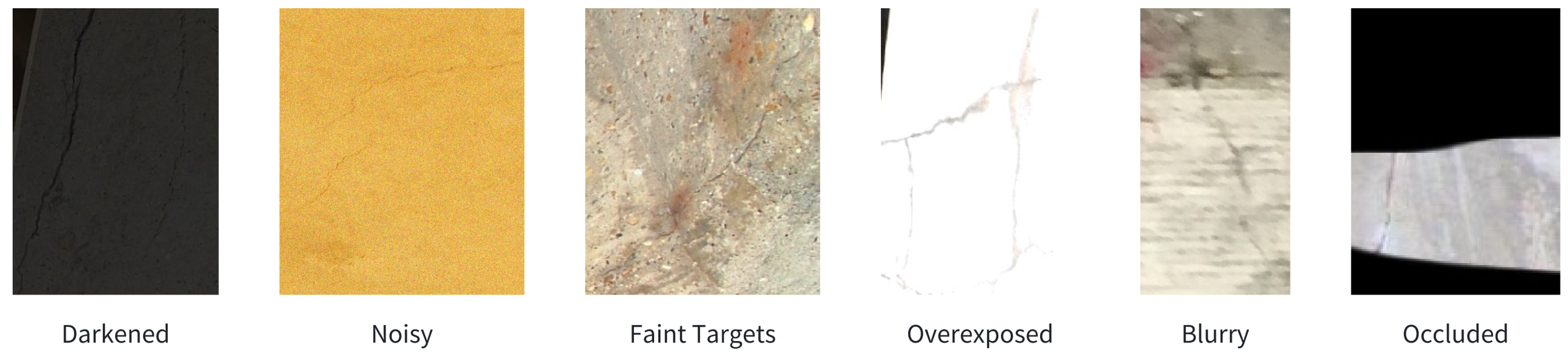
In practical industrial environments, we observe that images captured by drones often display significant variability and are frequently affected by six challenging conditions (the samples are shown in Figure 6), making classification considerably more difficult than in existing industrial defect datasets:

(1)

Darkened, where defects are obscured due to insufficient lighting or shadows, reducing visibility.

(2)

Noisy, which contain substantial interference from environmental factors such as texture patterns or imaging artifacts.

(3)

Faint Targets, where the defects are subtle and lack clear boundaries, making them difficult to distinguish from the surrounding material.

(4)

Overexposed, resulting from excessive lighting, which leads to the loss of critical defect details.

(5)

Blurry, caused by motion blur or focus issues during image capture, distorting the appearance of defects.

(6)

Occluded, where defects are partially hidden by other structures or objects, complicating their identification.

As illustrated in

Table 1. The details of our HDCD; $N_{train}$ is the number of training sets, and $N_{test}$ is the number of test sets.

Class	Example	Description	${\mathit{N}}_{\mathbf{train}}$	${\mathit{N}}_{\mathbf{test}}$
Crack		Linear fractures on the concrete surface	627	190
Efflorescence		White powdery deposits from dissolved salts	171	184
General		Minor surface irregularities or discoloration	219	71
No defect		Condition with no visible damage	344	111
Scaling		Peeling of thin concrete layers	102	99
Spalling		Chipping or breaking of the concrete surface	244	249
Total			1707	904

, our HDCD encompasses six image categories: crack, efflorescence, general, no defect, scaling, and spalling, with a total of 2418 images.

4.2. Implementation Details

For our challenging sample set, all categories except the unprocessed faint targets underwent manual secondary processing with reality-matching parameter adjustments: darkened images were generated through channel-wise multiplication with a darkness factor of 0.2 to reduce luminance; noisy samples incorporated additive Gaussian noise via np.random.normal at severity level 1; overexposed variants were created using ImageEnhance with a contrast amplification factor of 1.5; blurry images employed Gaussian blurring through cv2 with a 5 × 5 kernel; and occluded samples introduced random rectangular masks by zeroing pixel values.

Our proposed framework PPLF was implemented using PyTorch. All experiments were conducted on an NVIDIA 3060 GPU with 32 GB of memory. The model was implemented in Python 3.8 using PyTorch 1.10. The input query images were passed through three backbones: ResNet-50, EfficientNetV2-L, and ViT. All models were pre-trained on ImageNet, with ViT (base model p16) fine-tuned on ImageNet-21k. The input image size for all models was set to 224 × 224. Feature map dimensions extracted from the backbones were as follows: (a) ResNet-50: 2048 × 1 × 1 (channels, width, length), (b) EfficientNetV2-L: 1280 × 1 × 1, (c) ViT: 768 × 1 × 1. We trained ResNet-50 and EfficientNetV2-L for 100 epochs using the Adam optimizer, while ViT was trained with AdamW. The learning rate for all models was set to 0.001. After training, we loaded the optimal model parameters and tested them for 10 epochs on the test set.

For the loss function, during the backbone training stage, we used cross-entropy loss. In the overall framework training stage, we experimented with Label Smoothing Loss, which achieved an accuracy of 57.96%. However, the best performance was obtained using Mean Squared Error (MSE), achieving an accuracy of 60.51%.

For data augment, we used RandAugment with the parameters N = 4 (number of augmentation operations) and M = 9 (global magnitude), which provided the most satisfactory results.

4.3. The Effectiveness of Our Approach

The purpose of this experiment was to evaluate the effectiveness of our proposed PPLF. First, we assessed the performance of several widely used baseline models on our HDCD. We primarily selected three models: EfficientNetV2-L, ResNet-50, and ViT [41] as backbones, which represent diverse architectural paradigms (e.g., convolutional networks, residual learning, and transformer-based models). Furthermore, most existing concrete-defect-detection methods employ these models as a backbone [42,43,44,45], suggesting that they are recognized as valid for texture-level classification. To ensure fairness and comparability, we applied consistent data preprocessing procedures and evaluation criteria across all models. After loading the pre-trained optimal parameters for each backbone, we integrated our PPLF with the frozen backbones and conducted further training and testing.

Table 2. Comparison of backbone networks using the original methods versus our proposed framework. The accuracy and macro-F1 are with 95% confidence intervals.

Backbone	Method	Accuracy (%)	Macro-F1 (%)
ViT	None	$46.51\pm 0.33$	$41.60\pm 0.01$
	+PPLF	$\mathbf{48.96}\pm \mathbf{0.13}$	$\mathbf{48.03}\pm \mathbf{0.07}$
EfficientNetV2-L	None	$50.31\pm 0.24$	$46.81\pm 3.37$
	+PPLF	$\mathbf{54.21}\pm \mathbf{0.16}$	$47.28\pm 0.06$
ResNet-50	None	$53.51\pm 2.93$	$49.13\pm 2.57$
	+PPLF	$\mathbf{60.51}\pm \mathbf{2.16}$	$50.03\pm 1.87$

presents the comparative results of baseline models with and without our PPLF, evaluated through accuracy and macro-F1 score. The suboptimal performance of the baseline models on the HDCD highlights the inherent challenges of classifying bridge defect images, particularly due to their texture-level characteristics. Unlike high-level semantic features, texture-level defects such as cracks, spalling, and corrosion often exhibit subtle and irregular patterns, making them difficult to distinguish even for state-of-the-art models. This complexity is further exacerbated by real-world conditions such as lighting variations, occlusions, and background noise, which are prevalent in our test dataset.

The integration of PPLF consistently improved performance across all models, with ResNet-50 achieving the most substantial gain, increasing accuracy from 53.51% to 60.51%. This significant improvement can be attributed to the synergistic interaction between ResNet-50’s residual blocks and PPLF’s design. The architectural design of ResNet-50, characterized by hierarchical convolutional layers and residual skip connections, demonstrates a strong capability to capture local texture features, making it particularly effective for identifying the fine-grained and spatially localized patterns inherent in bridge defect imagery. PPLF enhances this alignment by prompt learning and feature fusion.

In contrast, ViT exhibited more modest gains, with accuracy increasing from 46.51% to 48.96%. ViT relies on self-attention mechanisms to model global dependencies between image patches. While this design excels in capturing high-level semantic relationships, it introduces two critical challenges for texture-level defect classification. First, the self-attention operation computes pairwise interactions between all patches, which may dilute the focus on localized defect regions (e.g., cracks spanning only 5–10 pixels). Second, ViT’s patch embedding layer imposes a rigid grid structure on input images, potentially disrupting subtle texture patterns that require sub-patch granularity. These architectural constraints are exacerbated by the limited scale of the HDCD, as transformers typically require pretraining on large datasets to stabilize gradient updates in attention layers. Consequently, even with data augmentation in PPLF, which enhances sample diversity through geometric and photometric transformations, ViT struggles to converge on discriminative features for fine-grained defects.

Meanwhile, EfficientNetV2-L’s accuracy in the HDCD improved from 50.31% to 54.21%. It employs compound scaling to balance depth, width, and resolution, optimizing computational efficiency through depthwise separable convolutions. However, this design reduces the capacity for hierarchical feature fusion, a key component of PPLF. Specifically, PPLF operates by aligning intermediate convolutional features with prototype vectors learned from defect patterns, a process that benefits from rich multi-scale representations. In EfficientNetV2-L, the depthwise convolution layers generate spatially sparse feature maps, limiting the granularity of prototype matching. Additionally, the model’s heavy reliance on squeeze-and-excitation modules prioritizes channel-wise attention over spatial localization, which conflicts with PPLF’s emphasis on defect-specific spatial prototypes.

Table 3. The computational efficiency of backbone networks, where (1) inference time is measured per individual image, and (2) training time is evaluated over 100 epochs.

Model	Participant Number (M)	FLOPs (G)	Input Size	Inference Time (ms)	Training Time (min)
ViT-B/16	86	17.6	224 × 224	25	153
EfficientNetV2-L	121	24.3	224 × 224	34	208
ResNet-50	25.5	4.1	224 × 224	15	78

presents the inference times of each model on our HDCD, benchmarked on an NVIDIA RTX 3060 GPU (32 GB memory). ResNet50 demonstrated the shortest inference time and training time while simultaneously achieving the highest metric performance in Table 2. These results collectively indicate that ResNet-50’s local feature extraction capability provides the optimal balance for PPLF implementation. While ViT’s global attention mechanisms and EfficientNetV2-L’s parameter efficiency present alternative approaches, PPLF maintains strong generalizability across all backbones, highlighting its robustness for texture-level defect classification.

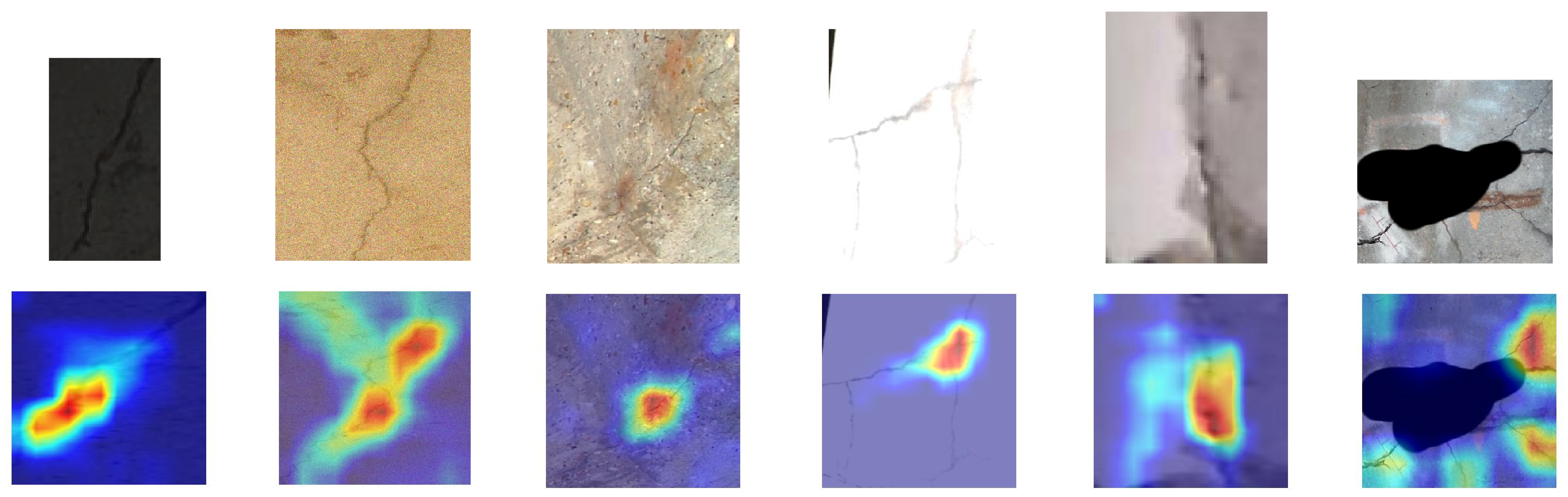
Figure 7 presents Grad-CAM visualizations of PPLF’s attention under six challenging conditions: darkened, noisy, faint targets, overexposed, blurry, and occluded. Using crack samples as representative cases, the results demonstrate PPLF’s consistent ability to localize defects accurately across all scenarios.

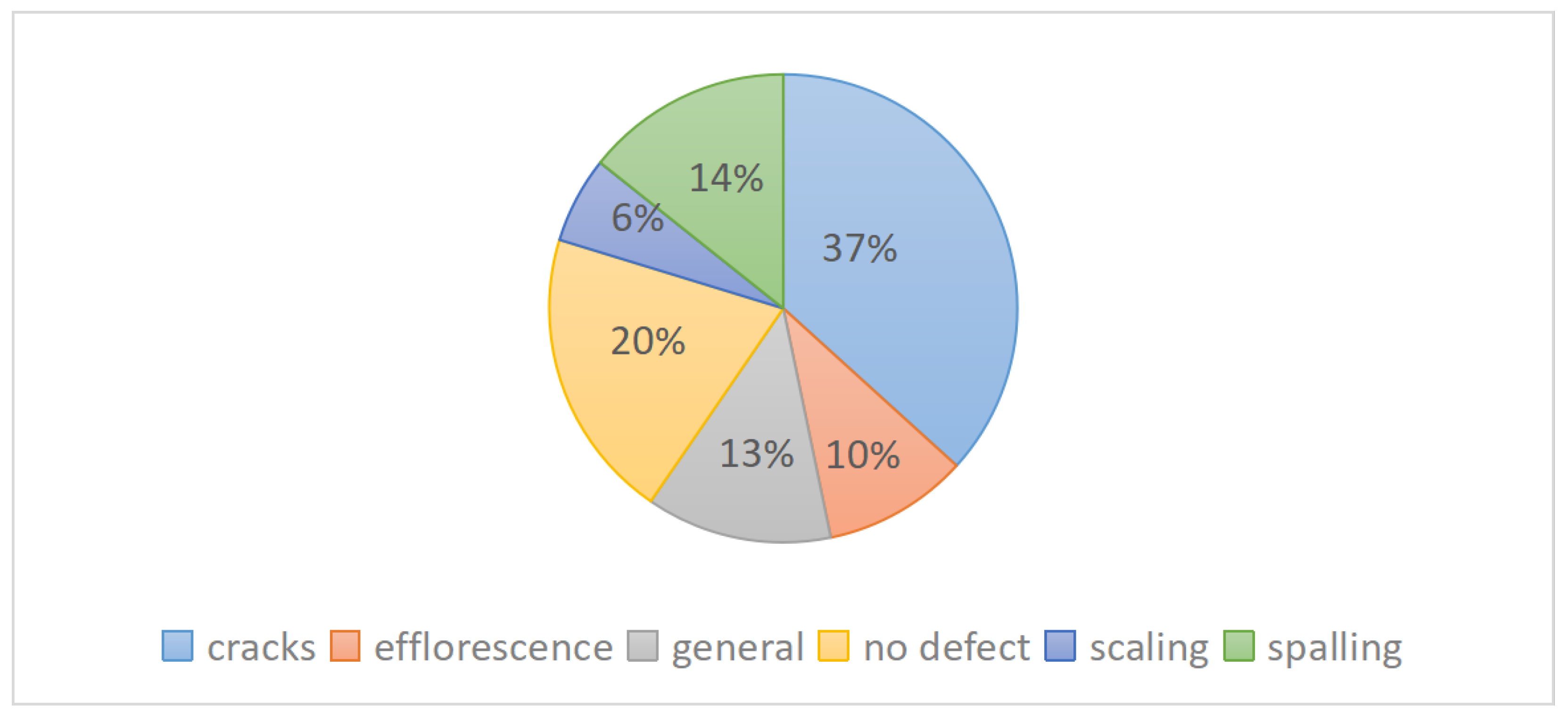
Although our model initially improves accuracy on hard samples, our dataset remains relatively small, containing only 2418 images. This is sparse compared to standard image classification datasets like ImageNet or CUB. And since defects are distributed in bridges with different degrees of commonness, some defects will be more prevalent, such as cracks, resulting in a varying number of images per category, which exacerbated the difficulty of our experiment. By analyzing the performance across precision, recall, and macro-F1 metrics, we observed variability in the results of our PPLF framework (using ResNet-50 as the backbone) for different defect categories; the results are shown in

Table 4. Using ResNet-50 as the backbone, our framework PPLF demonstrates its performance on the HDCD across different categories.

Class	Precision	Recall	Macro-F1
Crack	0.55	0.88	0.68
Efflorescence	0.80	0.40	0.54
General	0.40	0.49	0.44
No defect	0.49	0.77	0.60
Scaling	0.49	0.25	0.33
Spalling	0.64	0.50	0.56

.

The crack category exhibited the highest recall of 0.88, which means that the framework was able to identify 88% of the actual crack samples. This high recall is largely due to ResNet-50’s convolutional layers, which excel at capturing local linear patterns—a key characteristic of cracks. PPLF further enhances this capability by aligning intermediate features with prototype vectors representing crack textures, enabling robust localization even under noisy conditions. However, the precision of 0.55 suggests that only 55% of the samples predicted as cracks were actually cracks. Considering that the number of training sets for the crack category was 627, which was the largest number relative to the other categories as shown in Figure 8, it is likely that the model was overfitted during training for this category. This phenomenon arises because, during training, the model is exposed to a disproportionately large number of features in the crack compared to other samples. As a result, it may incorrectly classify other defects as cracks. In essence, the model for this category may have learned not only the meaningful patterns in the data but also the noise and random fluctuations, which are irrelevant and non-informative. The F1 score for the crack category was 0.68, which is a combination of precision and recall. Specifically, a high F1 score means that the model neither misses too many cracks that are actually present when predicting cracks (high recall), nor incorrectly identifies too many non-cracks as cracks (relatively high precision). This balance is especially important for crack classification, since too many false positives can lead to unnecessary inspections and repairs, while missed inspections can pose a safety hazard.

The Efflorescence category achieved the highest precision of 0.80, demonstrating the model’s ability to accurately identify efflorescence with 80% confidence. This high precision can be attributed to the unique visual characteristics of efflorescence (e.g., white, powdery appearance), which make it easier for ResNet-50’s hierarchical feature extraction to distinguish it from other defects. PPLF’s prototype vectors further enhance this capability by learning discriminative representations of efflorescence patterns. Conversely, the model performed poorly on the scaling category, particularly in recall, indicating that many actual scaling samples were missed. This underperformance can be attributed to the limited representation of scaling in the training data, preventing the model from learning sufficient information about this category.

4.4. Ablation Study

To validate the design choices of our method and model components for optimal efficiency and accuracy, we conducted ablation studies on the HDCD using ResNet-50 as the backbone network. The results presented in

Table 5. Results of ablation study of our model on our HDCD (the backbone is RelationNet-50). Acc (mean) and Acc (best) refer to the mean and maximum values, respectively, of accuracy on the hard sample set within 10 rounds (all values are in %).

Methods	Acc (Mean)	Acc (Best)	Precision	Recall	Macro-F1
Backbone	53.90	54.27	52.42	52.23	48.69
FFC	55.15	57.30	52.33	52.44	50.18
FFC + CERM	58.87	58.30	56.05	54.90	53.49

demonstrate that each proposed module contributes significantly to overall performance improvement.

The baseline model achieved a macro-F1 score of 48.69%, accompanied by a moderate accuracy at 53.90% and precision at 52.42%. This suboptimal performance highlights ResNet-50’s limitations in processing complex texture-level defects, particularly when distinguishing subtle inter-class variations such as cracks versus spalling or handling intra-class diversity like efflorescence patterns. These challenges demand finer-grained feature discrimination capabilities.

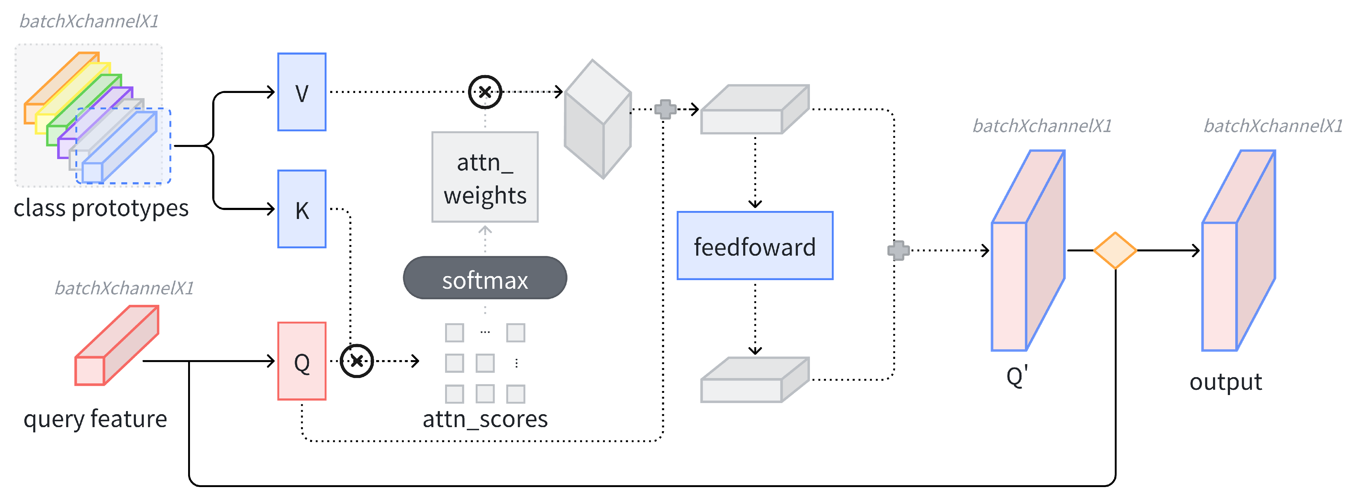
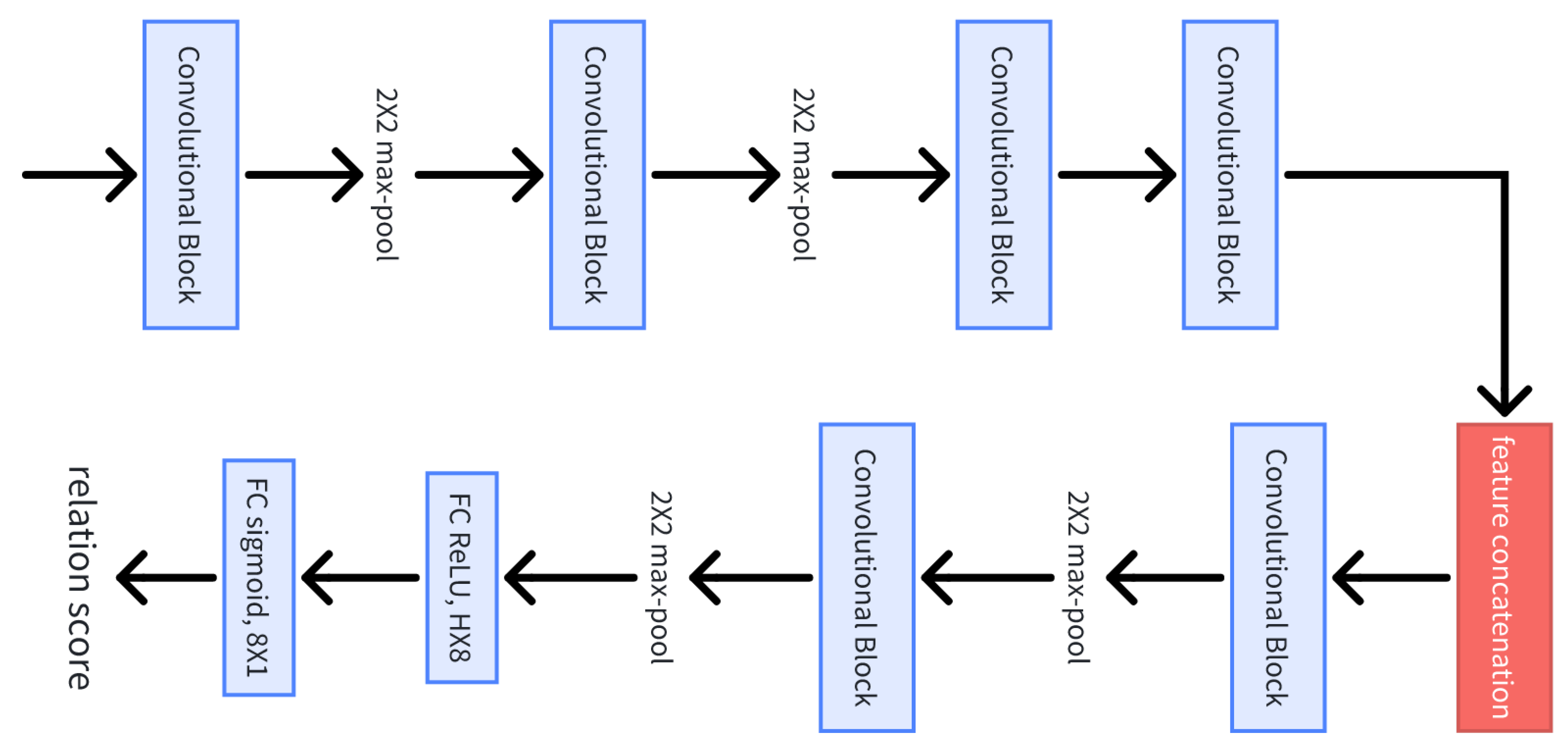
The introduction of the FFC elevated the average accuracy to 55.15% and macro-F1 to 50.18%. This component overcomes the backbone’s constraints by computing pairwise affinity matrices between feature maps from different convolutional stages. The accuracy gains confirm its capacity for resolving ambiguous cases through relational reasoning.

Further performance enhancements came from the CERM-enhanced FFC, which raised macro-F1 to 53.49% and average accuracy to 58.87%. This module dynamically integrates low-level texture features with high-level semantic embeddings. Such integration enables focused attention on discriminative local regions while filtering out irrelevant background noise. The concurrent improvement in both precision and recall metrics demonstrates the module’s dual capability to boost prediction confidence through context-aware localization while maintaining comprehensive defect coverage.

The ablation studies verify that both the FFC and CERM are indispensable. The former injects explicit relational inductive biases, while the latter enables hierarchical feature refinements. Together, they address the backbone’s limitations in texture-level defect classification.

4.5. Data Augmentation

According to Section 4.3, although our framework achieved good success, some problems with the data led to poor categorization results. Data augmentation is a technique for expanding a training set by creating variants of the original data, which increases data diversity through geometric transformations, color adjustments, noise injection, etc. Appropriate data enhancement methods can effectively solve the overfitting phenomenon of our model on cracks due to the problem of unbalanced datasets.

The comparison results are presented in

Table 6. Results of different data augmentation approaches combined with our model on our HDCD (the backbone is RelationNet-50).

Methods	Accuracy (%)	Macro-F1 (%)
None	58.87	53.49
RandomErasing	60.00	59.80
Cutmix&Mixup	59.04	54.40
BSR (all)	59.46	57.11
BSR (1,4)	60.13	55.19
TrivialAugmentWide	59.00	58.32
BSR (all) + Randaugment	60.08	58.01
Randaugment	60.51	59.89

. None refers to the method in Table 5 that uses ResNet-50 as the backbone and includes only the FFC and CERM. The data augmentation methods we employed include the following: (1) RandomErasing, which improved the accuracy to 60.51% by simulating occlusions (e.g., dirt, shadows) through random rectangular masking [46]. (2) Cutmix&Mixup: CutMix [47] and Mixup [48] are two popular data augment methods, both of which improve the generalization ability and robustness of a model by image blending and label interpolation. They had a limited efficacy (54.40% macro-F1), stemming from their semantic-level blending strategies, which conflict with texture-level defect detection. (3) BSR (Block Shuffle and Rotation), a novel input transformation-based attack [49]. BSR’s block shuffle and rotation introduces structured chaos by rearranging image regions, theoretically encouraging global context learning. In BSR (all), we quadrupled the entire dataset, which led to performance improvements but significantly increased training time with an accuracy of 59.46%. To optimize further, we focused on augmenting only the efflorescence and scaling categories, which had the fewest training samples. This approach yielded a slightly better accuracy (60.13%) than BSR (all). These methods inadvertently corrupt the discriminative texture features that PPLF’s prototype vectors rely on, explaining their suboptimal performance despite improving generalization in conventional classification tasks. However, façade defect classification relies more on texture, reducing their effectiveness. (4) TrivialAugmentWide’s random policy selection with a 59.00% accuracy introduces uncontrolled variations, such as extreme color jittering or over-rotation, which distorts subtle texture patterns [50]. (5) RandAugment achieved the highest accuracy, 60.51%, and macro-F1, 59.89%, by striking an optimal balance between diversity and consistency. It has two parameters: the number of enhancement operations N and a global enhancement magnitude M. By tuning the parameters, we finally found the most suitable parameters for our dataset and method to achieve the highest accuracy rate. (6) The combination of RandAugment and BSR (all) achieved only marginal improvements, with a 60.08% accuracy, as BSR’s spatial fragmentation counteracts RandAugment’s carefully calibrated transformations. This antagonism highlights the importance of a coherent augmentation design—strategies must complement rather than conflict with each other and the model’s inductive biases. Based on their performance, we ultimately integrated RandAugment as the data augmentation method into our PPLF.

In fact, we also made some substitutions and attempts in the FFC module and the CERM, such as replacing the CERM with the FMRM module to bi-directionally refactor prototype vectors and query vectors [51], bridging two cross-attentions, etc. These supplementary experiments are detailed in

Table 7. Results of different modules integrated into our method on our HDCD (the backbone is RelationNet-50, the data augmentation is randaugment).

Methods	Accuracy (%)	Macro-F1 (%)
None	53.90	48.69
CERM + CERM + FFC	59.39	52.78
FMRM + FFC	60.08	51.25
FMRM + CERM + FFC	60.03	52.22

. Some module combinations also yielded good results, but the framework was ultimately designed to prioritize the combination with the best overall performance.

The combination of the dual CERM with the FFC achieved an accuracy of 59.39% and macro-F1 of 52.78%. While this configuration improved over the baseline (+5.49% accuracy), its suboptimal F1 score suggests that stacking multiple CERM layers introduces feature redundancy. Specifically, the first CERM module refines low-level texture features by focusing on defect regions. The second CERM module, however, over-suppresses non-defective background regions, inadvertently removing contextual cues needed for inter-class relationship modeling in RelationNet. This tension between localized refinement and global dependency modeling explains the lower macro-F1 compared to configurations with fewer attention layers. The FMRM combined with the FFC achieved the highest accuracy but the lowest macro-F1 among the tested combinations. We hypothesize that FMRM operates by generating multi-scale feature representations, which improve the localization of texture anomalies. However, its recalibration mechanism, likely involving channel-wise reweighting, over-emphasizes high-frequency texture details, conflicting with RelationNet’s goal of learning smooth inter-class dependencies. Their full combination achieved a 60.03% accuracy and 52.22% macro-F1. FMRM prioritizes multi-scale feature multiplicity, which generates noisy intermediate representations. The CERM attempts to filter this noise but struggles to reconcile the conflicting goals of local refinement and global recalibration. RelationNet’s dependency graphs are, thus, trained on inconsistent features, limiting their ability to model robust inter-class relationships.

The FFC and CERM exhibit natural synergy—the former models global dependencies, while the latter refines local features. However, adding redundant or conflicting modules disrupts this balance.

5. Conclusions

In civil engineering projects, automated data collection often encounters complex working environments, resulting in challenging samples that degrade the performance of state-of-the-art (SOTA) methods. To address this, we developed the HDCD, which comprehensively incorporates six challenging conditions. Our evaluation revealed a significant performance drop on hard samples compared to ordinary ones, primarily due to the difficulty in capturing class-specific features under adverse conditions.

To mitigate these challenges, we propose the Prototypical Prompt Learning Framework (PPLF), which enhances defect recognition by performing a dynamic interaction between class prototype features and challenging sample features. This interaction improves the model’s focus on defect targets while reducing background interference. Experiments across three backbone networks demonstrated the PPLF’s robustness on our challenging test set, achieving consistent improvements over baseline methods.

However, several limitations and challenges remain: the PPLF’s performance partially relies on the quality of initial prototype vectors, which may be suboptimal for underrepresented defect categories. Our extensive heatmap analysis revealed that blurred inputs significantly scatter the model’s attention regions despite maintaining correct classification outcomes. This observation underscores two critical requirements for industrial UAV-based inspection: (1) stable image acquisition to minimize motion blur, and (2) sufficient pixel resolution in cropped subimages to preserve defect features. Although effective on the HDCD, the ability of the PPLF to generalize to entirely new challenging conditions (e.g., extreme weather or novel types of defects) requires further validation.

Despite these limitations, this study represents a novel application of prompt learning in bridge defect classification, advancing the safety and automation of bridge inspection processes. Future work will focus on optimizing the model’s architecture to address these challenges, such as developing adaptive prototype initialization strategies and lightweight interaction modules, further expanding its applicability in real-world engineering scenarios.