Rectifier Fault Diagnosis Using LTSA Optimization High-Dimensional Energy Entropy Feature

Abstract

In the electric locomotive traction transmission system, a four-quadrant rectifier has a high fault rate owing to the complicated control and bad operating conditions, and the fault directly affects the system’s safety and stability. To address such an issue, a rectifier fault diagnosis approach regarding a local tangent space alignment (LTSA) dimensionality reduction to optimize the high-dimensional energy entropy feature is proposed. Firstly, the fault signal is analyzed by using different wavelet functions through wavelet packet multi-resolution decomposition technology so as to extract the frequency band information of the signal. Each wavelet function corresponds to a specific frequency band; the energy–information entropy ratio of each frequency band coefficient is calculated, and then, the wavelet function and optimal frequency band, which are appropriate for the fault signal, are determined. Secondly, the energy entropy of each coefficient in the optimal frequency band is calculated to form the high-dimensional energy entropy feature. The LTSA algorithm is adopted to optimize the high-dimensional feature, through the fault sample number and clustering results, solve the difficulty of selecting the inherent dimension and nearest neighbor number in high-dimensional data, and obtain the simple and effective low-dimensional feature vector to describe the fault features, which reduces the conflict and redundancy between features. Finally, the optimized fault features are used as an input to the classifier support vector machine (SVM), and the fault types are obtained through training and testing. To validate the efficacy of the presented approach, it is tested from the aspects of noise environment, sample proportion and algorithm complexity, and compared with advanced methods. The results indicate that the proposed technique attains an average accuracy of 99.0625% in four-quadrant rectifier fault diagnosis. Under a different signal-to-noise ratio (SNR) and different training and test ratios, the average value after 30 diagnoses is better. Compared with other methods, this method shows a high diagnostic rate and strong robustness in terms of output voltage, noise, training and test ratio.

1. Introduction

A four-quadrant rectifier is an important electrical equipment in an electric locomotive, which works in both the rectifier state and the inverter state through pulse width modulation, and the power factor is close to 1 [1]. In the process of traction and regenerative braking, electric energy consumption is reduced and the conversion rate and utilization rate of electric energy are improved.

During the operation, the rectifier frequently encounters issues such as high temperature or pressure, and overcurrent, as well as overvoltage, that lead it to be prone to failure [2]. The fault will result in the distortion of input current and voltage and failure of regenerative braking, and seriously affect the safe operation of the train. Therefore, an efficient fault diagnosis method can effectively avoid the occurrence of train accidents and improve the operation and maintenance ability of trains.

The fault sources of a four-quadrant rectifier come from IGBTs and power diodes. The existing fault diagnosis methods mainly include a model-based method, a signal-based method and a data-driven method. The model-based approach is a traditional approach aimed at building mathematical models of actual systems. By detecting the difference between the measured signal and the model prediction signal, the fault diagnosis system has a fast response speed. The authors of [3] combined the mixed logic dynamic model of the system with the sliding mode observer to establish a state estimator and complete the IGBT open-circuit fault diagnosis. The authors of [4] used four kinds of observers to complete the IGBT open-circuit (OC) fault diagnosis. In [5], based on the known system parameters, a theoretical model was established, the excitation current output from the theoretical model was compared with the actual measured excitation current, and the diode open-circuit fault in the rectifier was detected. These model-based methods determine the actual fault features within the system and possess notable advantages in terms of diagnostic speed. However, depending on precise system parameters and models, the complexity of modeling and the uncertainty of parameters will affect the applicability of the model-based method. The signal-based method does not need a mathematical system model, and the symptoms and features of the tested signal are extracted by signal-processing technology to obtain the diagnosis results. The authors of [1] determined the threshold of each residual according to the analytical redundancy relationship under the rectifier fault condition and the mean and variance levels of each residual under normal conditions to complete the fault diagnosis of IGBT. The authors of [6] analyzed the instantaneous input voltage of the rectifier to detect and locate the OC fault of IGBT under different load conditions. The authors of [7] proposed an open-circuit fault diagnosis method for a three-level neutral-point-clamped rectifier, which uses the deviation between the actual reference voltage and the expected reference voltage to detect the open-circuit fault without a complicated calculation, accurate modeling, and additional hardware. Although these signal-based fault diagnosis methods can achieve high diagnostic accuracy, designing appropriate thresholds is rather difficult, which demands substantial prior knowledge and in-depth theoretical analysis of the system. Moreover, the performance degrades significantly when load fluctuations occur.

The data-driven approach avoids the dependence on the system model and the analysis of signal prior knowledge, and diagnoses the fault types through signal processing, feature extraction and pattern recognition, which has strong robustness and dynamic features [8]. In reality, within a noise setting, the fault signal exhibits nonlinear and non-stationarity features; as a result, the system’s modeling and signal analysis are constrained to a certain degree. Therefore, the data-driven method is more suitable for rectifier fault diagnosis. However, in order to capture the fault information completely from the nonlinear and non-stationary signals, the extracted fault feature dimension is too high. Excessive feature dimensions not only generate redundant information, but also complicate the feature space, greatly increasing the difficulty for identification, and affecting fault diagnosis accuracy. Therefore, in the data-driven approach, simple and sensitive fault features can lessen the pattern recognition computational burden to enhance the fault diagnosis rate.

To address the pattern recognition difficulty caused by high-dimensional fault features in fault diagnosis, dimension reduction technology [9] is usually used to simplify the complex features so as to enhance the fault diagnosis results. Principal Component Analysis (PCA) is a perfectly effective method to obtain low-dimensional feature samples from high-dimensional feature samples due to its outstanding advantages in dimensionality reduction and feature extraction. In the inverter system power switch open-circuit fault diagnosis, discrete Fourier transform (DFT) is used to extract the frequency domain features of the fault signal; then, the dimension of the features is reduced by PCA, and its contribution graph is used to locate the fault IGBT [10]. The authors of [11] propose the fault diagnosis of a wind energy conversion system based on the Hidden Markov model (HMM) and PCA; the features are extracted and selected by PCA, and the features are input into HMM classifier to improve the classification accuracy. However, as a linear dimensionality reduction algorithm, PCA determines the projection direction by maximizing the global variance in data, which makes it difficult to accurately capture the internal structure of data when dealing with nonlinear data, and it is easy to lose key local information. The Kernel Principal Component Analysis (KPCA) method expresses the nonlinear and multivariate properties of the system well [12]. The authors of [13] present an effective fault diagnosis technique in wind energy converter systems. The proposed method merges the benefits of KPCA and the bidirectional long short-term memory (BiLSTM) classifier. The KPCA is developed in order to select and extract the most efficient features and the final features after dimensionality reduction are fed to the BiLSTM to distinguish between different working modes. In marine pipeline corrosion degradation prediction based on monitoring data, using KPCA to reduce the dimension of the factors affecting pipeline corrosion can eliminate the redundant information in the original monitoring data and improve the efficiency of the prediction model [14]. However, the KPCA disadvantage is that the time and space complexity of calculating the kernel matrix is high, especially when processing large-scale data; the calculation cost is significantly increased, the choice of kernel function and related parameters is more sensitive, and different choices may lead to large differences in results. Although t-Distributed Stochastic Neighbor Embedding is good at dealing with nonlinear data, it mainly focuses on the local similarity of the data and distorts the global structure of the data in the process of dimensionality reduction.

The manifold learning algorithm demonstrates a remarkable capacity for extracting low-dimensional data structures from nonlinear high-dimensional data, and it has garnered extensive attention among numerous dimensionality reduction algorithms. The major aim of the manifold learning algorithm is to analyze the manifold topological structure of high-dimensional data, and to find the low-dimensional feature that best represents the operating state of the equipment. As the industrial scale continues to expand, the data exhibit nonlinear and high-dimensional features in order to solve the problem of dimensionality reduction in fault diagnosis. The authors of [15] provide an effective method for dimensionality reduction in fault diagnosis. LTSA integrated with a multi-distance adaptive order morphological filter fault diagnosis method first uses LTSA to retain local manifold structure to provide feature spatial data, then introduces cosine distance and dynamic time normalization distance into the distance error to improve classification accuracy, and finally determines the fault type according to the distance-matching results. By constructing the local tangent space of data points, LTSA can effectively preserve the local geometric structure of data and accurately adapt to the complex distribution characteristics of nonlinear fault signal. In [9], dimensionality reduction technology was adopted to extract fault features in analog circuit fault diagnosis, and a fault feature extraction algorithm combining LLE and diffusion maps (DMs) was proposed. In [16], the local linear embedding (LLE) algorithm was used to reduce the dimensionality of high-dimensional features, and the rectifier fault diagnosis result was improved. Although manifold learning theory has excellent performance in dimensionality reduction for nonlinear high-dimensional data, the selection of the intrinsic dimension d and the neighborhood points k in the process of dimensionality reduction faces many problems, such as complicated computation and strong limitations.

In view of the nonlinear and non-stationary fault data presented by the four-quadrant rectifier in the noise environment, the fault diagnosis research of the rectifier in this paper is carried out from three aspects: signal processing, feature extraction, and high-dimensional data dimensionality reduction. To obtain an efficient fault feature, it is necessary to consider not only effective signal decomposition but also the sensitivity of the features. Wavelet packet decomposition can not only achieve multi-resolution decomposition in the time–frequency domain, but also has certain robustness to noise. Entropy-based features can be used to characterize the nonlinear features resulting from the system’s transient alterations so as to quantify the dynamic changes in fault signals to distinguish various operating states, which exhibit outstanding clustering ability, high classification accuracy, and strong robustness. Due to the large amount of data and complex structure of nonlinear high-dimensional features, the calculation burden of the classifier is increased, and the result of the fault diagnosis is affected. Therefore, it is necessary to find a suitable dimensionality reduction algorithm for manifold learning. Simultaneously, determining the problem of selecting the intrinsic dimension d of data and the neighborhood points k is needed.

In this paper, a fault diagnosis technique regarding the local tangent space arrangement to optimize a high-dimensional energy entropy feature is proposed. Firstly, different wavelet functions are used to decompose the fault signal with multi-resolution to obtain different frequency band information. According to the energy–information entropy ratio (EIER) for each frequency band, the wavelet function appropriate for the fault signal is selected. The corresponding frequency band is the optimal frequency band, and each frequency band coefficient energy entropy is calculated. Secondly, the local tangent space alignment (LTSA) algorithm is adopted to fuse high-dimensional features through the fault sample number and clustering results, solve the difficulty of selecting the inherent dimension and neighborhood points number, and obtain the simple and effective low-dimensional feature for the fault features description, which reduces the conflict and redundancy between features. Finally, fault diagnosis of the four-quadrant rectifier is realized by a support vector machine (SVM). The main contributions are presented as follows:

(1) A novel approach that uses wavelet functions to conduct multi-resolution decomposition of nonlinear fault signals is proposed. By introducing the energy–information entropy ratio (EIER), the issue of which of the different wavelet functions can lead to inconsistent decomposition results for the same fault signal is resolved. This approach not only provides a systematic way to select the optimal wavelet function but also significantly improves the effectiveness of signal decomposition.

(2) A method combining energy entropy and LTSA is proposed, which not only considers the dynamics of energy and probability distribution in nonlinear fault signals, but also solves the instability of nonlinear signal features in data distribution, optimizes data distribution, and reduces the redundancy and conflict among features.

(3) An innovative approach to determine the inherent dimension and neighborhood points number in high-dimensional data is developed. By leveraging the number of fault samples and clustering results, the problem of parameter selection in high-dimensional datasets is solved. This method provides a practical and effective solution when dealing with similar high-dimensional data analysis problems.

(4) The fault diagnosis methods mentioned show remarkable diagnostic performance. Under different output voltages, the average diagnosis rate of 30 times for 15 fault modes is as high as 99% when the signal-to-noise ratio (SNR) is 50 dB. In addition, for different SNRs and different training and test ratios, the average diagnostic result is better after 30 fault diagnosis. Compared with other methods, this method shows a high diagnostic rate and strong robustness in terms of output voltage, noise, and the training-sample-to-test-sample ratio.

The rest of this paper is structured as follows: Section 2 provides a description of the four-quadrant rectifier system and an analysis of its fault modes. Section 3 details the algorithm for the extraction and optimization of high-dimensional energy entropy features. Section 4 conducts an analysis and a comparison of the fault diagnosis results. Section 5 concludes this study.

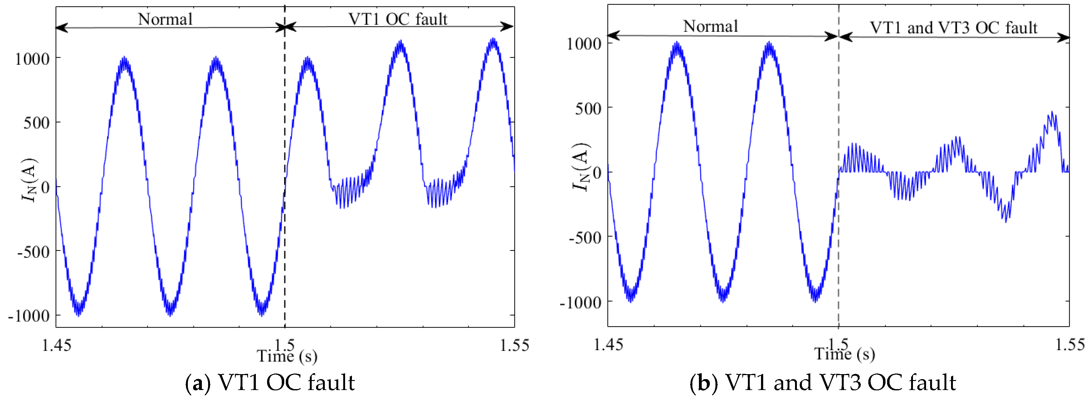
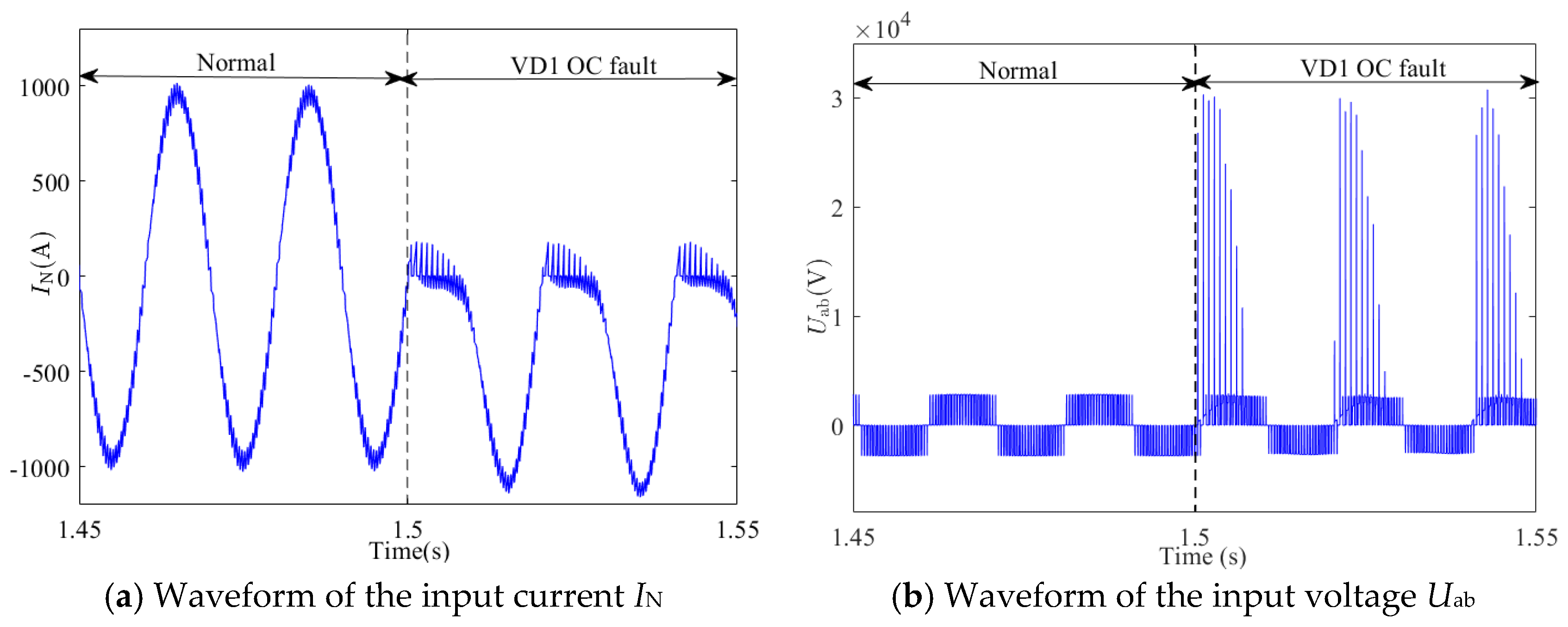
2. System Description and Fault Analysis

A four-quadrant rectifier is an important equipment for electric energy conversion in electric locomotives [17]. Its position and circuit structure in the traction transmission system are shown in Figure 1. When the output voltage is zero, the main transformer outputs 1450 V of alternating current (AC) voltage to supply power to the intermediate support capacitor until the output voltage is 2000 V, and, then, the traction winding directly supplies power to the four-quadrant rectifier until the output voltage is 2800 V, which is when the inverter begins to work.

The main sources of rectifier faults are open-circuit (OC) and short-circuit (SC) faults of the IGBT (represented by VTi) and power diode (represented by VDi). The SC fault is easily detected by the monitoring and protection device of the system [18]. OC faults cannot cause significant changes in the waveform for current and voltage; so, these cannot be detected for a short period of time, which may trigger secondary failures in other components, leading to more system losses [19]. Therefore, a four-quadrant rectifier fault diagnosis usually focuses on OC faults about IGBTs and power diodes.

On the basis of not adding sensors, the fault signal selects the existing input current sensor signal, and specifies that the direction of input current I_N flows towards the rectifier, I_N > 0; conversely, I_N < 0. OC faults are separately introduced into the IGBT and power diode, and then the impact of these OC faults on the system is analyzed.

IGBT single-OC fault and double-OC fault are injected at 1.5 s, as shown in Figure 2. The waveform of the current I_N before and after VT1 fault triggering is shown in Figure 2a. When I_N > 0, due to the anti-parallel action of diode VD1, the current passes through VD1, and the OC fault of VT1 has no effect on the rectifier’s operation. Therefore, the current I_N waveform remains unchanged during the first half-period after the fault occurs. When I_N < 0, the current I_N cannot pass through diode VD1, and the waveform is distorted for the second half period after the fault occurs. Therefore, the OC fault symptoms of VT1 occur only when I_N < 0. The waveforms of the current I_N before and after VT1 and VT3 faults trigger are shown in Figure 2b. When I_N > 0, the traction winding U_N charges the intermediate capacitor C_d through VT3. When an OC fault occurs in VT3, the current I_N distorts. When I_N < 0, the VT1 and VT3 OC fault hinder the energy feedback process. Therefore, whether I_N > 0 or I_N < 0, the OC fault of VT1 and VT3 will distort the waveform of current I_N, and the fault symptoms appear in the whole period. Therefore, IGBT single-OC and double-OC faults will cause the system to fail to work normally.

The single-OC fault of the power diode is injected at 1.5 s, as shown in Figure 3. The waveform of the current I_N before and after VD1 fault triggering is shown in Figure 3a. The input current I_N positive half-wave shape is distorted due to the fault of the rectifier branch. The waveform of the input voltage U_ab before and after the fault is triggered is shown in Figure 3b. The voltage U_ab waveform in the positive half-period is distorted, resulting in an instantaneous high voltage, which leads to an overvoltage fault in the IGBT, in a short span of time. Therefore, the diode OC fault will also affect the system’s normal operation, and in practical engineering, the probability of two power diodes failing at the same time is relatively low. Therefore, in the fault diagnosis of the four-quadrant rectifier power diode, only the single-OC fault of the diode is considered.

In the actual running process of the train, the IGBT or power diode may have an OC fault, and the different combinations of switching devices give rise to diverse fault modes, which, in turn, lead to distinct fault manifestations. A total of 15 OC fault modes (1 normal mode and 14 fault modes) of the four-quadrant rectifier are studied in this paper, and the fault modes corresponding to the fault types and their fault labels are shown in

Table 1. Fault mode.

Type	Mode	Label	Type	Mode	Label
Normal	Normal	1	Two IGBTs on the same half bridge	VT1VT3	8
Single IGBT	VT1	2		VT2VT4	9
	VT2	3	Two IGBTs on different half bridges	VT1VT4	10
	VT3	4		VT2VT3	11
	VT4	5	Single-power diode	VD1	12
Two IGBTs on the same bridge arm	VT1VT2	6		VD2	13
	VT3VT4	7		VD3	14
---	---	---		VD4	15

.

3. High-Dimensional Feature Extraction and Dimensionality Reduction Optimization

The simple and sensitive fault features help to reduce the computational burden of the classifier and improve the fault diagnosis result. The wavelet packet [20] is used to decompose nonlinear and non-stationary fault signals in multi-resolution, and the energy–information entropy ratio (EIER) is proposed to choose a wavelet function appropriate for signal decomposition so as to obtain the optimal frequency band information. A change in the failure mode will lead to a change in the signal energy value, and the entropy theory evaluates the probability of energy change. The smaller the energy entropy, the greater the probability of an energy value change, that is, the greater the possibility of a fault mode change. Therefore, the energy entropy feature is used to simultaneously characterize different fault modes from the distribution of values and probabilities. Local tangent space alignment (LTSA) [21] optimization for high-dimensional energy entropy feature is carried out in the data space to reduce outliers, reduce the dimensions of data, make the data appear scattered and tend to be normally distributed in the space, and eliminate redundancy and conflict among features.

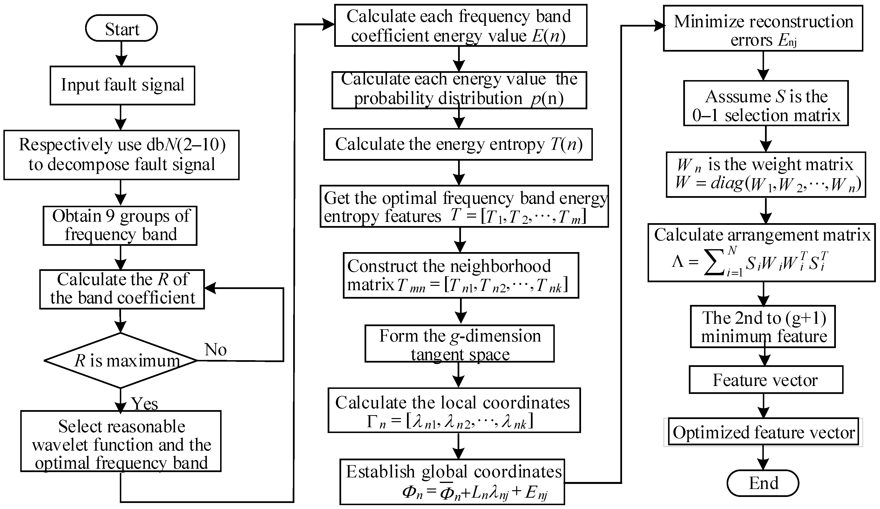
3.1. Feature Extraction Based on LTSA and Energy Entropy Algorithm

The process of high-dimensional energy entropy feature extraction and dimensionality reduction optimization algorithm, presented in Figure 4, proceeds with the following steps:

(1) Calculate the multiband coefficients of different wavelet functions. Assume fault signal, using 9 Daubechies wavelet functions commonly used for signal decomposition and reconstruction; the wavelet packet is utilized to decompose the fault signal, thereby acquiring 9 sets of frequency band information. And the 9 Daubechies wavelet functions are db2, db3, …, db10.

$$\left\{\begin{array}{c}{{\displaystyle f}}_{\mathrm{db}2}(r,m,n)=\left\{{{\displaystyle d}}_{r/\mathrm{db}2}^m(n)\right\}\\ \begin{array}{l}{{\displaystyle f}}_{\mathrm{db}3}(r,m,n)=\left\{{{\displaystyle d}}_{r/\mathrm{db}3}^m(n)\right\}\\ ⋮\end{array}\\ {{\displaystyle f}}_{\mathrm{db}N}(r,m,n)=\left\{{{\displaystyle d}}_{r/\mathrm{db}N}^m(n)\right\}\end{array}\right.$$

(1)

where ${{\displaystyle d}}_{r/\mathrm{db}N}^m(n)$ means that when dbN wavelet function is used, the n-th frequency band coefficient in m frequency bands is obtained after the signal is decomposed by r layer.

(2) Select the appropriate wavelet function. EIER is the frequency-band-coefficient-energy-to-information-entropy ratio, and takes the energy value variation and probability of fault mode into consideration. If a fault mode of the rectifier is Y_i and the probability of occurrence is P(Y_i), then the fault signal undergoes decomposition to obtain the frequency band coefficient energy value $V({{\displaystyle f}}_{\mathrm{db}N})$ and information entropy $H({{\displaystyle f}}_{\mathrm{db}N})$, and the corresponding frequency band EIER is R:

$$V({{\displaystyle f}}_{\mathrm{db}N})={\displaystyle \sum _{n=1}^M{{\displaystyle \left|{{\displaystyle d}}_{r/\mathrm{db}N}^m(n)\right|}}^2}$$

(2)

$$H({{\displaystyle f}}_{\mathrm{db}N})=-{\displaystyle \sum _r^{M}P({{\displaystyle Y}}_i)}{{\displaystyle \log }}_{2}P({{\displaystyle Y}}_i)$$

(3)

$$R={\displaystyle \frac{V({{\displaystyle f}}_{\mathrm{db}N})}{H({{\displaystyle f}}_{\mathrm{db}N})}}$$

(4)

For a fault signal, the larger the EIER is, the more suitable the chosen wavelet function is, and the frequency band obtained after decomposition is the optimal frequency band.

(3) Calculate the energy entropy features of the optimal frequency band. After the fault signal is decomposed by the wavelet packet r layer, m frequency band coefficients are obtained, and the energy entropy T(n) of each frequency band coefficient of the frequency band is calculated, where the energy value of the n-th frequency band coefficient is E(n), and the probability distribution is p(n).

$$E(n)={{\displaystyle \left|{{\displaystyle d}}_{r/\mathrm{db}N}^m(n)\right|}}^2$$

(5)

$$p(n)={\displaystyle \frac{{{\displaystyle E}}_n}{E({{\displaystyle f}}_{\mathrm{db}N})}}={\displaystyle \frac{{{\displaystyle \left|{{\displaystyle d}}_{r/\mathrm{db}N}^m(n)\right|}}^2}{{\displaystyle \sum _{n=1}^M{{\displaystyle E}}_n}}}$$

(6)

$$T(n)=-{\displaystyle \sum _{n=1}^{M}p(n)}{{\displaystyle \log }}_{2}p(n)$$

(7)

Therefore, utilizing the optimal wavelet function, the optimal frequency band energy entropy feature obtained by wavelet packet decomposition of the fault signal is T:

$$T=[{{\displaystyle T}}_1,{{\displaystyle T}}_2,\cdots ,{{\displaystyle T}}_m]$$

(8)

(4) Construct the neighborhood matrix of the energy entropy feature. Since the energy entropy feature T is an m-dimensional matrix, T_n is any data point in the matrix, and m is the data point number; the neighborhood points in each data are determined to be k, forming a neighborhood matrix.

$${{\displaystyle T}}_{mn}=[{{\displaystyle T}}_{n1},{{\displaystyle T}}_{n2},\cdots ,{{\displaystyle T}}_{nk}]$$

(9)

where T_nj is the j-th nearest neighbor of the n-th data point, n = 1, 2, …, N; j = 1, 2, …, k.

(5) Calculate the local coordinates. In the neighborhood matrix of data point T_n, the orthogonal basis Q_i is found to form the g-dimension tangent space. In the neighborhood, the orthogonal projection λ_nj of each point T_nj to the tangent space is calculated, and then the local coordinates of the neighborhood matrix T_mn are obtained as Γ_n:

$${{\displaystyle \mathrm{\Gamma }}}_n=[{{\displaystyle \lambda }}_{n1},{{\displaystyle \lambda }}_{n2},\cdots ,{{\displaystyle \lambda }}_{nk}]$$

(10)

(6) Establish global coordinates. Set the global coordinate $\Phi =[{{\displaystyle \Phi }}_1,{{\displaystyle \Phi }}_2,\cdots ,{{\displaystyle \Phi }}_N]$, and the local coordinate matrix of each data point in the energy entropy feature is arranged in the tangent space to obtain the global coordinate system. The global coordinate reflects the geometric structure of the local coordinate matrix, and the global coordinate should meet the following requirements:

$${{\displaystyle \Phi }}_n={{\displaystyle \overline{\Phi }}}_n+{{\displaystyle L}}_n{{\displaystyle \lambda }}_{nj}+{{\displaystyle {\rm E}}}_{nj}$$

(11)

where ${{\displaystyle L}}_n$ is the undetermined mapping matrix; ${{\displaystyle {\rm E}}}_{nj}$ is the reconstruction error; ${{\displaystyle \overline{\Phi }}}_n$ is the centralized matrix of ${{\displaystyle \Phi }}_n$.

(7) Calculate the permutation matrix. Assume that $S=[{{\displaystyle S}}_1,{{\displaystyle S}}_2,\cdots ,{{\displaystyle S}}_N]$, and S is the 0–1 selection matrix, and ${{\displaystyle W}}_n$ is the weight matrix of energy entropy feature data point T_n, that is, $W=diag({{\displaystyle W}}_1,{{\displaystyle W}}_2,\cdots ,{{\displaystyle W}}_n)$, and the arrangement matrix is $\mathrm{\Lambda }$:

$$\mathrm{\Lambda }={\displaystyle {\sum }_{i=1}^N{{\displaystyle S}}_i}{{\displaystyle W}}_i{{\displaystyle W}}_i^T{{\displaystyle S}}_i^T$$

(12)

(8) Minimize reconstruction errors. The feature vector corresponding to the 2nd to (g + 1) minimum feature value obtained by calculating the permutation matrix is each data point global coordinate in the energy entropy feature T, and is also the optimized feature vector $\Phi$.

$$\Phi =[{{\displaystyle \Phi }}_1,{{\displaystyle \Phi }}_2,\cdots ,{{\displaystyle \Phi }}_N]$$

(13)

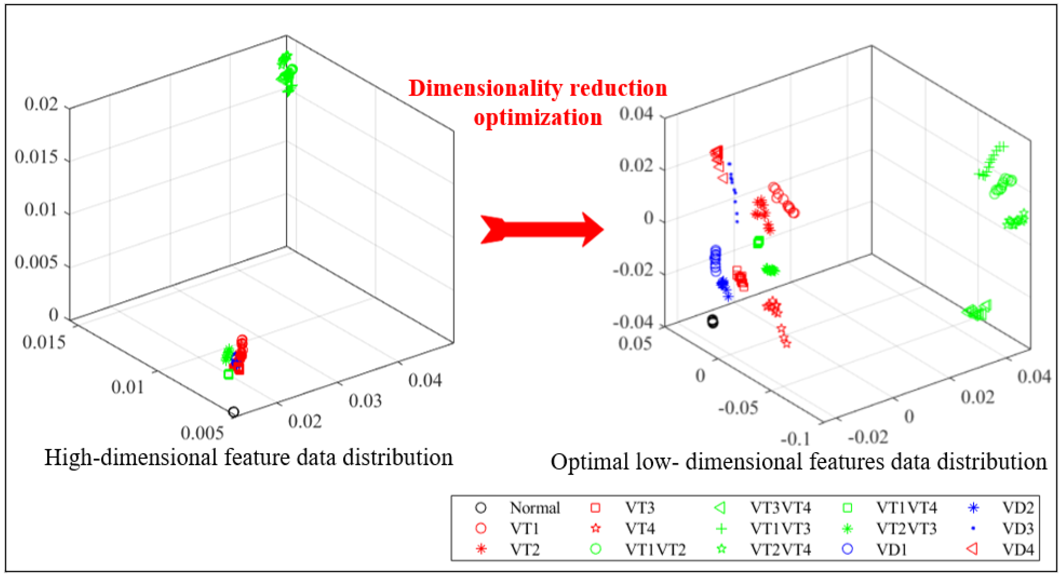
3.2. Optimal Low-Dimensional Feature Selection Based on DB Index

In the process of dimensionality reduction, due to the difference in neighborhood point k, the low-dimensional data after dimensionality reduction is different, which directly affects the result of fault diagnosis. According to the Davies Bouldin (DB) index [22], the better the clustering result, the more compact the data, the less redundancy and conflict between the features, and the better the dimensionality reduction effect. When the classification is known, that is, after the optimal clustering is determined, the DB_K values of a series of low-dimensional feature vectors are calculated, and the low-dimensional feature vector corresponding to the neighborhood point k with the smallest DB_K value is selected as the optimal feature vector. The basic contents of DB index are as follows:

(1) Calculate the average dispersion within the class.

$${{\displaystyle S}}_i={\displaystyle \frac{1}{\left|{{\displaystyle C}}_i\right|}}{\displaystyle \underset{X\in {{\displaystyle C}}_i}{\Sigma }‖X-{{\displaystyle Z}}_j‖}$$

(14)

where Z_j represents the class center of class C_i, and X represents the number of C_i class samples.

(2) Calculate the distance between classes.

$${{\displaystyle d}}_{ij}=‖{{\displaystyle Z}}_i-{{\displaystyle Z}}_j‖$$

(15)

Z_i and Z_j represent the class centers of C_i and C_j, respectively, and the distance between classes is represented by the distance between the two class centers.

(3) Calculate the DB_K value.

$${{\displaystyle DB}}_K={\displaystyle \frac{1}{K}}{\displaystyle \sum _{i=1}^K{{\displaystyle R}}_i}$$

(16)

$${{\displaystyle R}}_i=\underset{j=1,\dots ,k}{{\displaystyle \max }}{\displaystyle \frac{{{\displaystyle S}}_i+{{\displaystyle S}}_j}{{{\displaystyle d}}_{ij}}}$$

(17)

K is the number of categories. The smaller the DB_K, the better the clustering effect and dimensionality reduction effect [23].

3.3. Fault Diagnosis Method

Aiming at the fault diagnosis of a four-quadrant rectifier, a fault diagnosis method based on LTSA optimization of high-dimensional energy entropy feature is proposed, which includes data acquisition, signal processing, feature extraction, feature optimization and pattern recognition. The diagnostic block diagram is shown in Figure 5.

(1) Data acquisition. The input current signals of 15 fault modes under different working conditions are collected to form the original fault sample set.

(2) Data processing. It encompasses wavelet packet decomposition [24] and optimal frequency band selection. Wavelet packet decomposition is carried out using 9 Daubechies (dbN, N = 2, 3, …, 10). The wavelet function decomposes the signals of different working conditions and different fault modes, and obtains 9 groups of frequency band information of each fault mode. The optimal frequency band is selected according to each frequency band coefficient EIER, the corresponding frequency band information is the optimal frequency band suitable for the fault mode signal.

(3) Feature extraction. The energy entropy features T of the optimal frequency band are calculated, and the high-dimensional energy entropy features under different working conditions and different fault modes are extracted.

(4) Optimal low-dimensional feature selection. According to the fault mode, the intrinsic dimension is set as d = C − 1 (C is the number of fault modes). According to different neighborhood points k, the LTSA algorithm is used to reduce the dimensionality of high-dimensional features, and a series of low-dimensional features corresponding to the different neighborhood k are obtained. Through the DB_K index, the optimal low-dimensional features are selected from these low-dimensional features. According to the DB_K index, the DB_K index is the smallest, and the corresponding low-dimensional feature is the optimal low-dimensional energy entropy feature.

(5) Pattern recognition. The optimal fault feature vector is randomly divided into training samples and test samples, and the SVM [25] classifier is used for fault diagnosis.

4. Fault Diagnosis Results and Analysis

In order to verify the accuracy of the proposed method, a system simulation model was established.

Table 2. Four-quadrant rectifier main parameters.

Parameter	Name	Value	Unit
UN	Traction transformer secondary voltage	1450	V
LN	Traction transformer leakage inductance	2.3	mH
Udc	Traction rectifier output voltage	2800	V
Cd	Middle supporting capacitor	8	mF

shows the main parameters of the four-quadrant rectifier. The output voltage was set to change from 2000 V to 2800 V and to collect input current signals of 15 fault modes every 10 V. In order to simulate the noise environment, white noise with a signal-to-noise ratio (SNR) of 50 dB was added to the fault signal. Each fault mode has 81 sets of samples, and 15 fault modes have 81 × 15 = 1215 samples.

4.1. Optimal Wavelet Function Selection

Considering the fault features’ richness and the computational cost, a five-layer wavelet packet decomposition for the fault signal is conducted in this paper. The Daubechies (dbN) wavelet system, which is commonly used for signal decomposition and reconstruction, is selected. Nine kinds of dbN (N = 2–10) wavelet functions are used to decompose the signal; so, each sample and each fault mode have nine frequency bands. The energy–information entropy ratio of each band is calculated and compared; the ratio is the largest, indicating that the selected wavelet function is the best.

Table 3. Optimal wavelet function selection results for different fault modes.

Fault Mode	dbN	Fault Mode	dbN	Fault Mode	dbN
Normal	db5	VT1VT2	db6	VT2VT3	db3
VT1	db9	VT3VT4	db10	VD1	db2
VT2	db6	VT1VT3	db10	VD2	db2
VT3	db6	VT2VT4	db6	VD3	db2
VT4	db9	VT1VT4	db2	VD4	db2

shows the selection results of optimal wavelet functions for different fault modes when the output voltage is 2800 V and the SNR is 50 dB.

4.2. Extraction and Data Analysis of High-Dimensional Energy Entropy Feature

The fault signal is decomposed into 32 frequency bands by using the optimal wavelet function, and the energy entropy of each frequency band coefficient is calculated, that is, each fault mode has 32 energy entropy features. A line diagram and a box diagram are used to illustrate the energy entropy features and data distribution of each fault mode, as shown in Figure 6. When the rectifier output voltage is 2800 V, the line diagram of the energy entropy features for 15 fault modes is as shown in Figure 6a. The energy entropy features of different fault modes in the 1st to 5th frequency bands and the 13th frequency band are larger than those in other frequency bands, but the energy entropy of many fault modes overlaps with each other in the corresponding frequency bands, and it is impossible to accurately identify the fault type. The energy entropy features’ data distribution of the rectifier is analyzed through the box diagram, as shown in Figure 6b. There are a lot of outliers in the data, and all outliers are on the side of the larger value, indicating that the data distribution of energy entropy features is right-skewed and does not obey a normal distribution. The box diagram of the feature data of each fault mode is short, which means that many data points are distributed in a small range; each data point is similar, and the data are relatively concentrated, which is consistent with the analysis of the line diagram.

4.3. Dimensionality Reduction Optimization and Effect Analysis of High-Dimensional Feature

In the process of feature extraction, the feature data are normally distributed as much as possible, so that statistical inference and hypothesis verification can be better carried out. Although the energy entropy features obey a skewed distribution, the dispersion and deviation degree of data points are changed by dimensionality reduction technology, and the difference between data points is increased so that the data after dimensionality reduction can obey the normal or approximately normal distribution. Therefore, LTSA is used to reduce the dimensionality of the extracted high-dimensional energy entropy feature data to optimize data distribution. In order to avoid the difference in the data-intrinsic dimension, the difference in the neighborhood points’ number is calculated, considering the cost calculation and data portability. According to 15 fault types, the high-dimensional energy entropy feature is set to 14 dimensions.

The optimization effect of LTSA dimensionality reduction by the DB_K value is evaluated, and a reasonable neighborhood points number k is determined. The smaller the DB_K value of the sample, the higher the clustering quality and the better the dimensionality reduction effect. According to the different neighborhood points k, the DB_K value of the corresponding low-dimensional feature obtained after the dimensionality reduction in the high-dimensional feature is as shown in Figure 7. When k is 400, the DB_K value of the corresponding low-dimensional feature is the smallest, and the clustering effect is the best. Therefore, the low-dimensional feature corresponding to k is 400 is the optimal low-dimensional energy entropy feature.

For a high-dimensional energy entropy feature, the low-dimensional energy entropy features and data distribution after dimensionality reduction optimization are shown in Figure 8. The optimal low-dimensional energy entropy features are numerically dispersed, as shown in Figure 8a. The box diagram was used to analyze the data distribution of the optimized energy entropy feature, as shown in Figure 8b; after optimization, the outliers are obviously reduced, and the feature data obey an approximately normal distribution. The energy entropy feature has one or two outliers apart from the normal, VT2VT4 and VD1, but the outliers are significantly reduced, and the outliers of other fault modes are eliminated. The results of dimensionality reduction and optimization show that the distribution of feature data of each fault mode is optimized, the box diagram of the data is longer, the standard deviation and variance are increased, and the deviation degree of the data is weakened. The difference between the data points increases from the centralized state to the dispersed state. In terms of the symmetry of special data, data distribution is slightly skewed except for the upper and lower lengths of normal; VT1VT3, VT2VT4, VD1 and VD2 differ greatly. The upper and lower lengths of other fault modes are about equal, and the feature data are considered to have a symmetrical distribution.

By visualizing the classification effect of high-dimensional data, the optimization effect of the proposed method on dimensionality reduction in high-dimensional feature is verified. Three dimensions are arbitrarily selected from high-dimensional feature vectors to realize the visualization of high-dimensional data. Figure 9 shows the data distribution information before and after dimensionality reduction in high-dimensional features through the scatter plot.

As shown in Figure 9, due to the large amount of redundant information among high-dimensional features, various features are interrelated, and the sample data of fault types overlap each other, which makes it difficult to distinguish these, and the clustering effect is not ideal. This shows that the high-dimensional multi-domain features extracted are not conducive to fault diagnosis. The LTSA algorithm is used to obtain the optimal low-dimensional feature vector (1215 × 14). From the scatterplot, the overlap between fault-type data essentially disappears after dimensionality reduction optimization, and the clustering effect is good. However, the sample points in each fault type overlap and need to be further classified by the classifier. The scatterplot results show that the algorithm based on LTSA is effective for dimensionality reduction in a high-dimensional energy entropy feature.

4.4. Analysis of Diagnostic Results

In this paper, a support vector machine (SVM) is used as the fault feature classifier. When an SVM is used for nonlinear classification, the input data can be mapped to a high-dimensional space so that linear classification can be performed in that high-dimensional space. The kernel function is introduced to solve the problem of heavy computation in A high-dimensional space. Common kernel functions include the linear kernel function, the polynomial kernel function, the Radian Basis Function (RBF), and the Sigmoid kernel function. The linear kernel function is suitable for linear fractional data, which can be classified directly in the original feature space, and the calculation is simple and efficient. Polynomial kernel functions are suitable for cases where the data become linearly separable after polynomial feature extension. The Sigmoid kernel function is suitable for some applications that combine an SVM with neural networks. A Radian Basis Function (RBF) is suitable for most nonlinear data and has strong generalization ability. In view of the excellent performance of the RBF kernel function in practical applications, this paper selects the RBF as the kernel function, and uses the search and cross-validation method to determine the optimal value of penalty parameter C and kernel coefficient γ, two important parameters for SVM performance.

For 1215 fault samples containing 50 dB of white noise, 729 optimized fault samples of energy entropy features were randomly set as training samples. An SVM was used to compare the remaining samples as test samples with the actual output results, and the average diagnosis rate was taken as the evaluation index. After running for 30 times, the average diagnosis rate was 99.0625%. The average diagnosis results of each fault mode are shown in

Table 4. Each fault mode average diagnostic results.

Fault Mode	Average Accuracy	Fault Mode	Average Accuracy	Fault Mode	Average Accuracy
Normal	100%	VT1VT2	100%	VT2VT3	100%
VT1	100%	VT3VT4	100%	VD1	96.25%
VT2	99.7917%	VT1VT3	100%	VD2	98.026%
VT3	100%	VT2VT4	100%	VD3	95.1%
VT4	100%	VT1VT4	100%	VD4	96.77%

. Among the 486 random test samples, the average diagnosis rate of IGBT OC faults, except VT2 (99.7917%), is 100%, indicating that the proposed method has a good fault diagnosis effect for both single-OC faults and double-OC faults of IGBT. Although the fault diagnosis rate of the diode is lower than that of the IGBT, the diagnostic result is still high, indicating that the proposed method has higher diagnostic results for both IGBT and power diode OC faults.

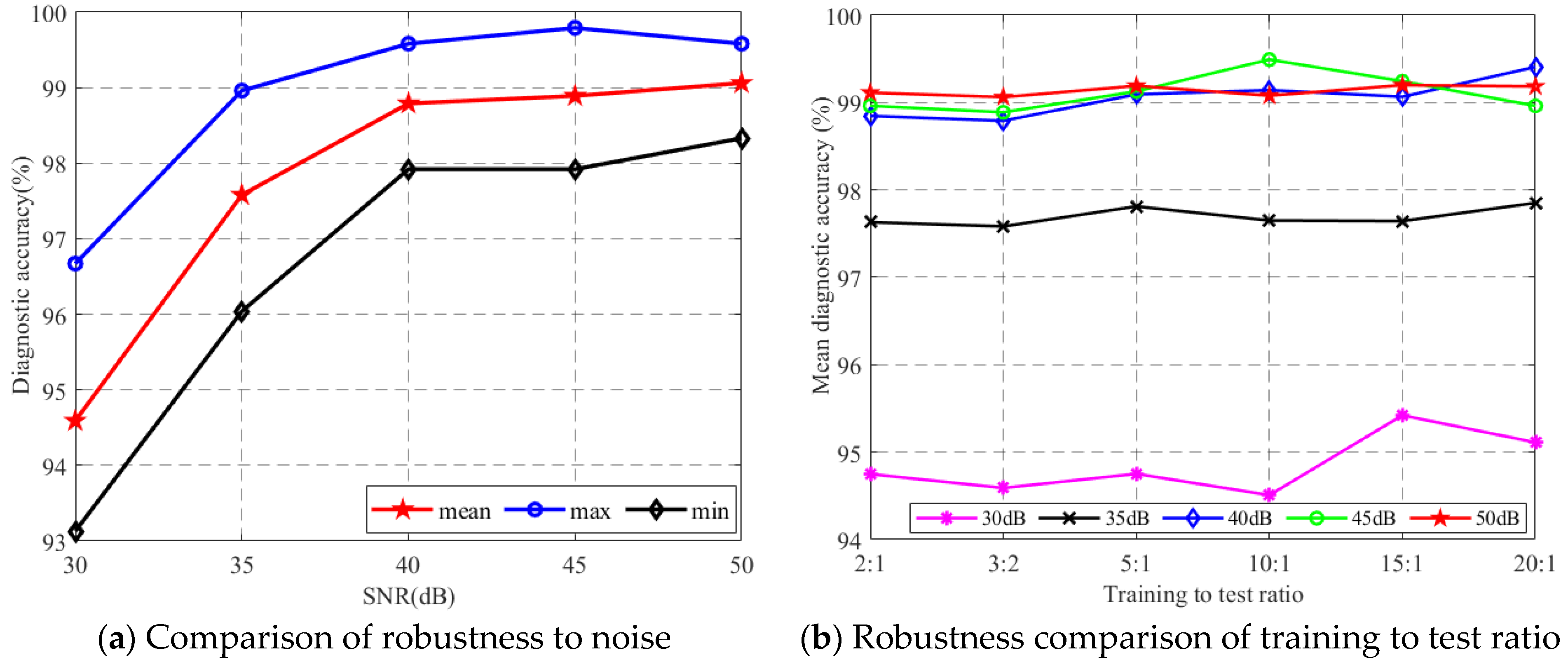
4.5. Robustness Verification and Analysis

In order to verify the robustness of the proposed method, different noise environments and different training to test ratios are analyzed. White noise with an SNR of 30 dB, 35 dB, 40 dB, 45 dB and 50 dB was added to the original signal, and the training-sample-to-test-sample ratios of data with different SNRs are set as 2:1, 3:2, 5:1, 10:1, 15:1 and 20:1, respectively. The robustness analysis results after running the proposed method 30 times are shown in Figure 10. When the SNR is 30 dB, as shown in Figure 10a, the average value after 30 diagnoses is 94.5903%, the maximum value is 96.6667%, and the minimum value is 93.1250%. With the increase in the SNR, the diagnostic results are all better than 30 dB, indicating that the proposed method has strong robustness to noise. When the training-sample-to-test-sample ratio is 3:2, the average diagnostic result is lower than that of other ratios, but the corresponding diagnostic rate is higher, as shown in Figure 10b, which is 94.5903%, 97.5833%, 98.7917%, 98.8889%, 99.0625%, respectively. Therefore, this method is also robust to the training-sample-to-test-sample ratio.

4.6. Decomposition Levels Analysis

In order to verify the rationality of five-layer signal decomposition, four-layer and six-layer decomposition are carried out on the data containing 50 dB, 45 dB and 40 dB white noise. After decomposition, fault diagnosis is carried out according to the proposed method, and each dataset is run 30 times. The maximum, average and minimum values of diagnostic accuracy are shown in

Table 5. Decomposition layers and diagnostic result.

Decomposition Layers	SNR (dB)	Mean (%)	Max (%)	Min (%)
4-layer	40	95.7778	97.5	94.375
	45	95.6875	97.5	93.9583
	50	95.944	97.5	94.583
5-layer	40	98.7917	99.5833	97.9167
	45	98.8889	99.7917	97.9167
	50	99.0625	99.5833	98.3333
6-layer	40	98.9167	99.3750	97.7083
	45	98.7708	99.5833	97.50
	50	98.9584	99.7917	98.125

. In the study of the number of decomposition layers, it was found that when six-layer decomposition is carried out, the average diagnostic result under noise of 40 dB is 98.9167%, and the maximum diagnostic result under noise of 50 dB is 99.7917%, but the diagnostic results in other cases were lower than the accuracy of the five-layer decomposition. Therefore, considering the degree of fault feature mining and the calculation cost, this paper finally chooses five-layer decomposition as the optimal scheme.

4.7. Algorithm Complexity Comparison

In terms of algorithm complexity, feature dimensionality reduction time, training time and diagnosis time, computation burden, and average diagnosis accuracy rate, 30 diagnoses are taken as evaluation indexes, as shown in

Table 6. Algorithm complexity comparison.

Algorithm	Dimensionality Reduction Time (s)	Training Time (s)/ Diagnosis Time (s)	Computation Burden (Parameter)	Accuracy (%)
Energy entropy feature	---	83.6324/0.0209	---	55.3681
PCA	0.0165	53.8707/0.034	Target dimensionality	57.5000
KPCA	0.6511	53.9517/0.0152	Target dimension, kernel function	52.7083
ISOMAP	126.7947	54.2798/0.0148	Target dimension, neighborhood points	53.1250
LTSA	124.4325	55.0171/0.0066	Target dimension, neighborhood points	99.0625

. In terms of computational burden, several dimensionality reduction algorithms all involve the target dimension. Although PCA does not require other parameters, PCA has a poor fusion effect on nonlinear data. While the KPCA and ISOMAP algorithms are suitable for dimensionality reduction in nonlinear data, KPCA has a great dependence on kernel function, which affects the accuracy of the diagnosis, and ISOMAP relies on geodesic distance approximation calculations. When the data sample distribution is uneven, there are noise or outliers, making it easy to construct an unreasonable neighbor map and to cause a large deviation in the geodesic distance estimation, which further affects the dimension reduction effect. Compared with the energy entropy features before optimization, the three algorithms all shorten the training and diagnosis time. Although the training time is almost the same, the diagnosis time of LTSA is the shortest. In terms of dimensionality reduction time, although the dimensionality reduction time of LTSA is longer, it can accurately optimize fault features; so, the average accuracy of fault diagnosis is the highest.

Figure 11 shows the advantages of the LTSA dimensionality reduction algorithm based on the DBK index in terms of “diagnosis time” and “diagnosis accuracy”. Because the LTSA algorithm arranges and aligns the local tangent space of each data point in high-dimensional data, it optimizes data distribution, facilitates classification by the classifier, and improves the diagnosis rate.

4.8. Comparison with Advanced Methods

In order to further explain the superiority of the proposed method, the results are compared with those of several advanced methods, as shown in

Table 7. Comparison with advanced methods.

Methods	Condition Change	Reliability	Training-Sample-to-Test-Sample Ratio	Noise Level	Accuracy
WPD-LTSA-SVM	Output current	Average run of 30 times	3:2	30 dB	94.5903%
PCA-HMM [11]	Not mentioned	Not mentioned	1:1	Data with noise	93.61%
MEMD-FE-AFSA-SVM [26]	Wind speed	Average run of 30 times	3:2	30 dB	95.5758%
Optimized-DBN [27]	Output current	Average run of 200 times	4:1	No noise	98.43%
RF [28]	Input current	Not mentioned	2:1	No noise	98.32%
WDD-CNN [29]	Load torque	Not mentioned	4:1	No noise	99.47%
				Data with noise	96.65%

.

In [26], under the same comparative conditions, the authors carry out multiple-empirical-mode decomposition (MEMD) on fault signals, extract fuzzy entropy (FE) eigenvalues, optimize the support vector machine (SVM) with the help of the artificial fish swarm algorithm (AFSA), and finally realize IGBT open-circuit fault diagnosis. The diagnosis rate is based on SVM optimization. It is only 0.9855% higher than that of the proposed method and does not take into account the failure of the diode. In [11], features are extracted and selected through PCA, and the features are input into the HMM classifier. The diagnostic accuracy is only 93.61%, and the level of noise is not indicated. The authors of [27] use the beetle antennae search algorithm’s optimized deep belief network (DBN) to diagnose a single-IGBT open-circuit fault in the rectifier. In [28], the open-circuit fault of IGBT in the PWM rectifier is analyzed, and it is pointed out that the occurrence of fault characteristics is related to the fault location and time. Then, a fault diagnosis for the PWM rectifier using random forest technology with transient synthetic features is proposed. In [27,28], the study of noise robustness is lacking, and the diagnostic accuracy is low. In [29], Wavelet Domain Denoising (WDD) and convolutional neural network (CNN) are used in the open-circuit fault diagnosis of IGBT in a wind power converter. The method uses deep learning, but the diagnostic performance is not ideal. The diagnostic rate of this method is only 96.65% in the case of noise. Although the diagnostic rate can reach 99.47% in the case of no noise, the ratio of the training samples to the test samples is 4:1, and reliability research is not mentioned. Therefore, the method proposed in this paper has good stability, strong robustness and a high diagnostic rate.

5. Conclusions

A fault diagnosis approach regarding LTSA optimization of a high-dimensional energy entropy feature is proposed for a rectifier. The multi-resolution decomposition of the nonlinear fault signal is realized by using the wavelet function, and the optimal frequency band is selected by using the energy–information entropy ratio, which solves the problem that different wavelet functions have different effects on the decomposition of the same fault signal and affect the accuracy of feature extraction. Considering the dynamic change in the energy of the nonlinear fault signal and its probability, energy entropy is taken as the fault features. LTSA is carried out to make the feature data tend to normal distribution and effectively reduce the outliers in the data. Through this spatial position optimization, the redundancy and conflict between multiple features are eliminated, the problem of nonlinear signal features being unstable in data distribution is solved, and a more robust and reliable basis for fault diagnosis is provided. Under different output voltages, the average diagnosis rate of 30 times for 15 fault modes is as high as 99%. In addition, for different noise levels and training and test sample ratios, the average diagnosis rate was over 94%. Compared with algorithm complexity, the proposed method not only has excellent diagnostic performance, but also shows strong robustness and can effectively cope with a variety of conditions.

References

1. Li, X.; Xu, J.; Chen, Z.; Xu, S.; Liu, K. Real-time fault diagnosis of pulse rectifier in traction system based on structural model. IEEE Trans. Intell. Transp. Syst. 2020, 23, 2130–2143. [Google Scholar] [CrossRef]
2. Liang, J.; Mao, X. Rectifier Fault Diagnosis Based on Euclidean Norm Fusion Multi-Frequency Bands and Multi-Scale Permutation Entropy. Electronics 2025, 14, 612. [Google Scholar] [CrossRef]
3. Xie, D.; Ge, X. A state estimator-based approach for open-circuit fault diagnosis in single-phase cascaded H-bridge rectifiers. IEEE Trans. Ind. Appl. 2018, 55, 1608–1618. [Google Scholar] [CrossRef]
4. Hu, K.; Liu, Z.; Iannuzzo, F.; Blaabjerg, F. Simple and effective open switch fault diagnosis of single-phase PWM rectifier. Microelectron. Reliab. 2018, 88, 423–427. [Google Scholar]
5. Mahtani, K.; Guerrero, J.M.; Beites, L.F.; Platero, C.A. Application of a Model-Based Method to the Online Detection of Rotating Rectifier Faults in Brushless Synchronous Machines. Machines 2023, 11, 223. [Google Scholar] [CrossRef]
6. Arehpanahi, M.; Entekhabi, A.M. A New Technique for Online Open Switch Fault Detection and Location in Single-phase Pulse Width Modulation Rectifier. Int. J. Eng. 2022, 35, 1759–1764. [Google Scholar] [CrossRef]
7. Chen, M.; He, Y. Open-circuit fault diagnosis in NPC rectifiers using reference voltage deviation and incorporating fault-tolerant control. IEEE Trans. Power Electron. 2023, 39, 1514–1526. [Google Scholar]
8. Xia, X.; Ning, P. Fault Diagnosis of Frequency Control System Based on FFT. In Proceedings of the 2019 22nd International Conference on Electrical Machines and Systems (ICEMS), Harbin, China, 11–14 August 2019; pp. 1–5. [Google Scholar]
9. Yuan, Z.; He, Y.; Yuan, L.; Chen, P.; Cheng, Z. An efficient feature extraction approach based on manifold learning for analogue circuits fault diagnosis. Analog. Integr. Circuits Signal Process. 2020, 102, 237–252. [Google Scholar]
10. Sun, X.; Song, C.; Zhang, Y.; Sha, X.; Diao, N. An open-circuit fault diagnosis algorithm based on signal normalization preprocessing for motor drive inverter. IEEE Trans. Instrum. Meas. 2023, 72, 3513712. [Google Scholar]
11. Kouadri, A.; Hajji, M.; Harkat, M.F.; Abodayeh, K.; Mansouri, M.; Nounou, H.; Nounou, M. Hidden Markov model based principal component analysis for intelligent fault diagnosis of wind energy converter systems. Renew. Energy 2020, 150, 598–606. [Google Scholar]
12. Fezai, R.; Dhibi, K.; Mansouri, M.; Trabelsi, M.; Hajji, M.; Bouzrara, K.; Nounou, H.; Nounou, M. Effective random forest-based fault detection and diagnosis for wind energy conversion systems. IEEE Sens. J. 2020, 21, 6914–6921. [Google Scholar]
13. Yahyaoui, Z.; Hajji, M.; Mansouri, M.; Abodayeh, K.; Bouzrara, K.; Nounou, H. Effective Fault Detection and Diagnosis for Power Converters in Wind Turbine Systems Using KPCA-Based BiLSTM. Energies 2022, 15, 6127. [Google Scholar] [CrossRef]
14. Li, X.; Jia, R.; Zhang, R.; Yang, S.; Chen, G. A KPCA-BRANN based data-driven approach to model corrosion degradation of subsea oil pipelines. Reliab. Eng. Syst. Saf. 2022, 219, 108231. [Google Scholar]
15. Zhang, N.; Xu, Y.; Zhu, Q.X.; He, Y.L. Improved multi-distance ARMF integrated with LTSA based pattern matching method and its application in fault diagnosis. IEEE Trans. Autom. Sci. Eng. 2023, 21, 3461–3471. [Google Scholar]
16. Mao, X.; Dong, H. Feature Fusion Based on Locally Linear Embedding in Fault Diagnosis of A Single-Phase PWM Rectifier. In Proceedings of the 2023 7th International Conference on Smart Grid and Smart Cities (ICSGSC), Lanzhou, China, 22–24 September 2023; pp. 94–100. [Google Scholar]
17. Gonzalez-Jimenez, D.; Del-Olmo, J.; Poza, J.; Garramiola, F.; Madina, P. Data-driven fault diagnosis for electric drives: A review. Sensors 2021, 21, 4024. [Google Scholar] [CrossRef]
18. Liang, J.; Zhang, K.; Al-Durra, A.; Zhou, D. A novel fault diagnostic method in power converters for wind power generation system. Appl. Energy 2020, 266, 114851. [Google Scholar]
19. Liang, J.; Zhang, K.; Al-Durra, A.; Zhou, D. A multi-information fusion algorithm to fault diagnosis of power converter in wind power generation systems. IEEE Trans. Ind. Inform. 2023, 20, 1167–1179. [Google Scholar] [CrossRef]
20. Liang, Y.; Zhang, J.; Shi, Z.; Zhao, H.; Wang, Y.; Xing, Y.; Zhang, X.; Wang, Y.; Zhu, H. A Fault Identification Method of Hybrid HVDC System Based on Wavelet Packet Energy Spectrum and CNN. Electronics 2024, 13, 2788. [Google Scholar] [CrossRef]
21. Lu, N.; Zhang, G.; Xiao, Z.; Malik, O.P. Feature extraction based on adaptive multiwavelets and LTSA for rotating machinery fault diagnosis. Shock Vib. 2019, 2019, 1201084. [Google Scholar]
22. Ros, F.; Riad, R.; Guillaume, S. PDBI: A partitioning Davies-Bouldin index for clustering evaluation. Neurocomputing 2023, 528, 178–199. [Google Scholar]
23. Zhong, X.; Shih, F.Y. Automatic Image Pixel Clustering based on Mussels Wandering Optimization. Int. J. Pattern Recognit. Artif. Intell. 2021, 35, 2154005. [Google Scholar]
24. Kuai, Z.; Huang, G. Fault diagnosis of diesel engine valve clearance based on wavelet packet decomposition and neural networks. Electronics 2023, 12, 353. [Google Scholar] [CrossRef]
25. Liang, J.; Zhang, K. A robust fault diagnosis scheme for converter in wind turbine systems. Electronics 2023, 12, 1597. [Google Scholar] [CrossRef]
26. Liang, J.; Zhang, K. A new hybrid fault diagnosis method for wind energy converters. Electronics 2023, 12, 1263. [Google Scholar] [CrossRef]
27. Du, B.; He, Y.; Zhang, Y. Open-circuit fault diagnosis of three-phase PWM rectifier using beetle antennae search algorithm optimized deep belief network. Electronics 2020, 9, 1570. [Google Scholar] [CrossRef]
28. Kou, L.; Liu, C.; Cai, G.W.; Zhou, J.N.; Yuan, Q.D. Data-driven design of fault diagnosis for three-phase PWM rectifier using random forests technique with transient synthetic features. IET Power Electron. 2020, 13, 3571–3579. [Google Scholar]
29. Liu, J.; Wang, J.; Yu, W.; Wang, Z.; Zhong, G.A. Open-circuit fault diagnosis of traction inverter based on improved convolutional neural network. Journal of Physics: Conference Series. IOP Publ. 2020, 1633, 012099. [Google Scholar]
Figure 1. The position and circuit structure of the rectifier in the traction transmission system.
Electronics 14 01405 g001
Figure 2. IGBT OC fault.
Electronics 14 01405 g002
Figure 3. VD1 OC fault.
Electronics 14 01405 g003
Figure 4. Flow chart of high-dimensional feature extraction and dimensionality reduction algorithm.
Electronics 14 01405 g004
Figure 5. Fault diagnosis block diagram.
Electronics 14 01405 g005
Figure 6. Energy entropy features and data distribution.
Electronics 14 01405 g006
Figure 7. DBK values of low-dimensional features corresponding to different neighborhood points k.
Electronics 14 01405 g007
Figure 8. Energy entropy features and data distribution after optimization.
Electronics 14 01405 g008
Figure 9. Fault features’ data scatter plot.
Electronics 14 01405 g009
Figure 10. Robustness analysis and comparison.
Electronics 14 01405 g010
Figure 11. Advantages of the LTSA algorithm based on the DBK index.
Electronics 14 01405 g011