Deep Reinforcement Learning for UAV Target Search and Continuous Tracking in Complex Environments with Gaussian Process Regression and Prior Policy Embedding

Abstract

In recent years, unmanned aerial vehicles (UAVs) have shown substantial application value in continuous target tracking tasks in complex environments. Due to the target’s movement behavior and the complexities of the surrounding environment, the UAV is prone to losing track of the target. To tackle this issue, this paper presents a reinforcement learning (RL) approach that combines UAV target search and tracking. During the target search phase, spatial information entropy is employed to guide the UAV in avoiding redundant searches, thus enhancing information acquisition efficiency. In the event of target loss, Gaussian process regression (GPR) is employed to predict the target trajectory, thereby reducing the time needed for target re-localization. In addition, to address sample efficiency limitations in conventional RL, a Kolmogorov–Arnold networks-based deep deterministic policy gradient (KbDDPG) algorithm with prior policy embedding is proposed for controller training.Simulation results demonstrate that the proposed method outperforms traditional methods in target search and tracking tasks within complex environments. It improves the UAV’s ability to re-locate the target after loss. The proposed KbDDPG efficiently leverages prior policy, leading to accelerated convergence and enhanced performance.

1. Introduction

In recent years, the rapid advancement of unmanned aerial vehicle (UAV) technology has significantly enhanced its application in search and tracking tasks. Owing to their high mobility, broad application spectrum, and cost-effectiveness, UAVs have been extensively used in disaster relief, environmental monitoring, and military reconnaissance [1,2,3,4,5]. Several conventional algorithms have been extensively integrated into UAV operations. For instance, the coverage path planning method divides the working area into sub-regions and explores them with simple back-and-forth motions to ensure full scene coverage and complete target search [6]. The method of artificial potential field creates a virtual attraction field at the target’s location and a repulsion field at the obstacle’s location, allowing the UAV to track the target under combined forces [7]. The genetic algorithm designs an appropriate encoding method and termination criteria, constructs a fitness function, and effectively performs genetic operations, such as selection, crossover, and mutation, to determine the UAV’s flight path [8]. However, in dynamic and complex environments, efficiently searching for and tracking moving targets remains a challenging problem, particularly when the UAV’s field of view (FOV) is limited, the target moves quickly, and obstacles cause interference. First, the UAV must be capable of avoiding environmental obstacles during search and target tracking to prevent collisions. Second, it should autonomously plan the optimal search path to maximize coverage. In addition, the UAV must be robust and flexible enough to adapt to various environments. Lastly, due to factors such as sensor failures and target occlusion by the environment, target-detection algorithms may not provide fully reliable results in a short time. This necessitates the UAV having predictive capabilities for target movement.

The emergence of reinforcement learning (RL) methods has attracted increasing attention. RL is modeled as a Markov decision process (MDP), where the RL agent observes the environment’s state, makes decisions accordingly, interacts with the environment, and receives reward feedback to inform better actions [9]. To enhance the ability of RL to address complex tasks, researchers have integrated it with deep learning, leading to the development of deep reinforcement learning (DRL) [10]. DRL utilizes neural networks to approximate value or policy functions, enabling optimization of network parameters during agent-environment interactions, thus maximizing cumulative rewards. DRL has demonstrated significant success across several domains, including competitive gaming, smart manufacturing, and transportation systems [11,12,13].

The advent of deep reinforcement learning has offered new solutions for addressing UAV target search and tracking challenges in dynamic and complex environments [14]. For example, Yuanyuan Sheng et al. proposed a DRL-based UAV autonomous navigation algorithm that establishes a dynamic reward function and a novel state-space representation method to solve the UAV’s autonomous path planning problem in high-density and highly dynamic environments [15]. Yongfeng Yin et al. tackled the problem of weak obstacle avoidance capability in UAV target tracking by proposing an innovative reinforcement learning method with attention guidance, enabling the UAV’s decision-making to shift between navigation and obstacle avoidance tasks based on changes in the environment [16]. Haobin Shi et al. proposed an end-to-end DRL navigation strategy that leverages curiosity to encourage the agent to explore previously unvisited environmental states, addressing the problem of map-less navigation in complex environments with sparse rewards [17]. However, these methods generally assume that the target’s location is known or that the target is static, which limits the system’s adaptability and generality for many real-world tasks. Therefore, Mei Liu et al. proposed a two-stage method for mobile target search and tracking in unknown environments, dividing the task into search and tracking phases and training the controller for each phase using a deep deterministic policy gradient algorithm with three critic networks [18]. Despite its advantages, this method lacks sufficient research on task switching, particularly in handling target loss. Once a target is lost, quickly re-localizing it becomes difficult, which makes long-term target tracking in complex environments challenging. To address the issue of target loss, Tian Wang et al. proposed a quantum probability model, which records the probability of the target in a discrete grid and updates the probability based on UAV observations and target movement to search for the lost target [19]. Yanyu Cui et al. developed an action decision-occlusion handling network based on deep reinforcement learning, using temporal and spatial contexts, object appearance models, and motion vectors to provide information on the occluded target, thus achieving target tracking under occlusion [20]. Although the above methods have made significant progress in target relocation after loss, most of these approaches are designed for relatively simple scenarios or require detailed target information, which limits their applicability in complex real-world environments. Moreover, reinforcement learning models typically require continuous interaction with the environment to achieve convergence. Unfortunately, these models are often inefficient in terms of sample utilization [21]. In particular, in UAV applications, training directly in the real world requires significant time and may damage the equipment [22]. One common approach is learning from demonstration (LfD), where experience is obtained from experts to reduce the need for training samples in real-world settings [23,24,25]. Nevertheless, LfD requires obtaining expert data, and the learning performance is largely dependent on the quality of the expert data. Additionally, in reinforcement learning applications, we often have prior information about the problem, but this knowledge is seldom leveraged by reinforcement learning algorithms. Therefore, Chao Wang et al. proposed an algorithm called non-expert-assisted deep reinforcement learning, which uses both prior and learned policy to jointly construct the behavior policy, successfully guiding UAVs to complete navigation tasks under sparse rewards [26]. Dawei Wang et al. proposed a two-stage multi-UAV collision avoidance method based on reinforcement learning. In the first stage, supervised training is used to encourage agents to follow prior policy, and in the second stage, policy gradients are employed to further refine the strategy [27]. The aforementioned methods effectively utilized prior policy in reinforcement learning, but they required certain rule-based guidance or staged training, leading to redundant training processes, which further inspired us to design a more novel training approach to utilizing prior policy.

To address the above issue, we propose a deep reinforcement learning method that accomplishes the two major tasks of target searching and target tracking, which improves the training efficiency of reinforcement learning through prior policy embedding. Specifically, we extend the concept of spatial information entropy and use it to compute rewards that guide the UAV’s target search [28]. Upon locating the target, the UAV transitions from search mode to tracking mode and commences tracking the target. When the UAV loses the target, it utilizes the information collected during tracking and applies Gaussian process regression (GPR) to forecast the target’s future trajectory, offering a probable target location [29]. This approach offers potential target locations, thereby substantially diminishing the time needed for the UAV to reacquire the target. As soon as the target re-enters the FOV, the UAV resumes the tracking task. This strategy, which integrates prediction and search, effectively enhances re-localization efficiency after target loss, addressing the limitations of conventional single-task methods in such scenarios. During the algorithm training phase, inspired by Kolmogorov–Arnold Networks (KANs) [30], we designed a novel method of utilizing prior policy and propose the KANs-based deep deterministic policy gradient (KbDDPG) algorithm. The introduction of KANs enables prior policy to be embedded into the policy network, guiding training with the prior policy, which enhances the reinforcement learning training speed and further improves the UAV’s target search and tracking performance. The main contributions of this study are:

• We propose an integrated decision-making framework for UAV search and tracking based on deep reinforcement learning, which significantly improves the efficiency of target search. It solves the re-localization problem after target loss, thereby achieving continuous target tracking.
• We design a deep deterministic policy gradient algorithm, KbDDPG, based on Kolmogorov–Arnold networks, which uses prior policy embedding to significantly accelerate the algorithm’s convergence rate.
• The proposed method is validated through extensive simulations in complex environments, demonstrating its effectiveness and superiority. Compared to existing DRL algorithms, our approach outperforms them in target search and tracking tasks.

The structure of the paper is as follows. Section 2 introduces the main model for UAV target search and tracking. Section 3 elaborates on the proposed method, covering trajectory prediction based on GPR, the extended spatial information entropy model, and the DRL algorithm based on KANs. Section 4 conducts experiment and analyzes the results. Finally, Section 5 concludes the paper and explores future research directions.

2. System Model

In this paper, we consider a target search and tracking system that consists of UAV equipped with gimbaled cameras. We assume that the UAV can use a gimbaled camera to capture the position information of obstacles and moving targets within its FOV. The UAV must search for targets within the area without collision and continuously track them upon detection. The following sections introduce the main model for the UAV target search and tracking task. To apply RL methods, we have made some simplifications and assumptions in constructing the dynamics model. These assumptions are clear and reasonable under suitable conditions.

2.1. UAV Dynamics Model

This study focuses on a UAV with adequate maneuverability and sensing capabilities. For UAVs, altitude information is crucial during actual flight, but in many target search and tracking tasks, UAVs are often set to fly at a fixed altitude. When verifying and optimizing the performance of the algorithm in this paper, using two-dimensional modeling helps focus on the UAV’s search, tracking, and relocalization problems without having to simultaneously solve the complex altitude control issue. Therefore, we modeled the UAV as a simple mass point and assumed it flies at a fixed altitude. The UAV operates in a two-dimensional grid model, where each cell represents a possible position. We use grid partitioning to simplify the spatial representation, facilitating the design of subsequent algorithms. A 2D space of size $M\times M$ is constructed, with the set of all possible spatial positions defined as:

$$\mathbb{M}=\left\{(x,y)|0\le x,y<M\right\}$$

(1)

At time $t(t\in \left\{1,\dots ,T\right\})$, let $p_u^t=(x_u^t,y_u^t)$ denote the UAV’s position and  $u^t=(a_u^t,{\omega }_u^t)$ denote the control inputs, where $a_u^t$ represents acceleration and ${\omega }_u^t$ represents the rate of change in the UAV’s heading angle. The dynamic equation for a UAV at discrete time intervals is as follows:

$$\left\{\begin{array}{c}{x}_u^{t+1}=x_u^t+v_u^{t+1}·\cos \left({\theta }_u^{t+1}\right)·\Delta t\hfill \\ y_u^{t+1}=y_u^t+v_u^{t+1}·\sin \left({\theta }_u^{t+1}\right)·\Delta t\hfill \\ v_u^{t+1}=v_u^t+a_u^t·\Delta t\hfill \\ {\theta }_u^{t+1}={\theta }_u^t+{\omega }_u^t·\Delta t\hfill \end{array}\right.$$

(2)

where ${\theta }_u^t$ denotes the heading angle and $v_u^t$ represents the velocity of the UAV in the direction of the heading angle.

In this context, ${\omega }_u^t$ is used to control the change in the UAV’s angle. However, the actual control inputs for a real UAV are typically represented by accelerations. To ensure the actions are reasonable, during simulations, we have imposed limits on the variation range of the control input ${\omega }_u^t$ to ensure that the acceleration range is within the maneuverability capabilities of a real UAV.

The UAV observes targets and obstacles using its onboard sensors. The sensor’s FOV covers a circular area, where R represents the maximum sensing range. The UAV’s FOV at time t and position $x,y$ is expressed as a set:

$${\mathbb{F}}_t=\left\{(x_i,y_i)\in \mathbb{M}|\sqrt{{(x_u^t-x_i)}^2+{(y_u^t-y_i)}^2}<R\right\}$$

(3)

To reduce the computational complexity of the model, the complex transformation from imagery to positional data is omitted. It is assumed that the UAV can directly obtain the relative positions of the target and obstacles. Using ${\rho }_g^t$ and ${\varphi }_g^t$ to represent the distance and relative angle, the target’s relative position within the UAV’s FOV is given by $L_g^t=({\rho }_g^t,{\varphi }_g^t)$, and the closest obstacle’s relative position is given by $L_o^t=({\rho }_o^t,{\varphi }_o^t)$. Given that in real-world applications, sensor measurements are inevitably influenced by noise and uncertainty. To address this, we incorporated sensor measurement noise into the model. The observed target position is expressed as ${\tilde{L}}_g^t=L_g^t+n_g,n_g\sim N(0,{\sigma }_g^{2}I)$, where ${\sigma }_g$ represents the standard deviation of uncertainty in the target’s relative position measurement, and I is the identity matrix. The observed obstacle position is denoted as ${\tilde{L}}_o^t=L_o^t+n_o,n_o\sim N(0,{\sigma }_o^{2}I)$, with ${\sigma }_o$ indicating the standard deviation of uncertainty in the obstacle measurement. This approach to modeling target and obstacle positions not only simplifies computational complexity but also facilitates easier transfer to real-world environments, ensuring high adaptability for both simulations and real UAV missions. During each simulation episode, the UAV and target start at random positions. The episode ends when the UAV either collides with an obstacle or reaches the maximum number of steps T.

2.2. Environment Model

The environment model is shown in Figure 1. We assume that during UAV search and tracking missions, various obstacles are present. This paper introduces irregular polygons as approximations of obstacles. The positions of obstacles that the UAV cannot occupy are defined by the set $\mathbb{Z}$:

$$\mathbb{Z}=\left\{(x_i^z,y_i^z)\in \mathbb{M}|i=1,\dots ,Z\right\}$$

(4)

During the target search and tracking process, the UAV must avoid obstacles to ensure operational safety. Additionally, there are line-of-sight occluded zones in the environment through which both the target and UAV can pass, but the UAV’s sensors cannot detect targets entering these areas. The line-of-sight occlusion zones are defined by the set $\mathbb{B}$:

$$\mathbb{B}=\left\{(x_i^b,y_i^b)\in \mathbb{M}|i=1,\dots ,B\right\}$$

(5)

The position of the target at time step t is represented as $p_g^t=(x_g^t,y_g^t)$, and the movement of the target is controlled by the vector $u_g^t=(a_g^t,{\omega }_g^t)$. The $u_g^t$ has L possible values, and the set of possible values is denoted by $\mathbb{L}=\left\{u_1,\dots ,u_L\right\}$. Thus, $u_g^t$ is expressed as a Markov chain with a finite set of states and state transition probabilities $p_{ij}=p(u_g^t=u_j|u_g^{t-1}=u_i)$, $i,j\in \left\{1,\dots ,L\right\}$, The state transition probability is given by the following formula:

$$P_{ij}=\left\{\begin{array}{cc}{P}_l,\hfill & \mathrm{if}i=j\hfill \\ {\displaystyle \frac{P_{ij}(1-p_l)}{L-1}},\hfill & \mathrm{if}i\ne j\hfill \end{array}\right.$$

(6)

By setting a higher $p_l$ value to simulate the target’s movement pattern, meaning the target’s control inputs tend to remain unchanged. Let $v_g^t$ denote the target’s velocity. The target’s motion equation is expressed as:

$$\left\{\begin{array}{c}{x}_g^{t+1}=x_g^t+v_g^{t+1}·\cos \left({\theta }_g^{t+1}\right)·\Delta t\hfill \\ y_g^{t+1}=y_g^t+v_g^{t+1}·\sin \left({\theta }_g^{t+1}\right)·\Delta t\hfill \\ v_g^{t+1}=v_g^t+a_g^t·\Delta t\hfill \\ {\theta }_g^{t+1}={\theta }_g^t+({\omega }_g^t+{\omega }_{avoid}^t)·\Delta t\hfill \end{array}\right.$$

(7)

We apply the velocity obstacle method to assist the target in avoiding obstacles [31]. Here, ${\omega }_{avoid}^t$ denotes the avoidance angular velocity, which modifies the target’s velocity to steer away from velocity obstacles and prevent collisions. Failed avoidance trajectories are discarded during this process.

3. Method

This section begins by modeling the target search and tracking problem using the MDP. We extend the concept of spatial information entropy to enlarge the UAV’s search range. To mitigate target loss during tracking, a trajectory prediction method based on GPR is proposed. Lastly, we introduce the KbDDPG algorithm.

3.1. Problem Statement

In UAV target search and tracking tasks, the problem is often modeled as a MDP. The MDP model comprises a five-tuple $(S,A,P,R,\gamma )$.

The state space S represents the set of all possible states. In this task, the state input includes the processed historical trajectory of the UAV, as well as the observed positions of obstacles and targets. Next, we will introduce the process of state extraction. The historical trajectory processing function is defined as $f_s:{\mathbb{M}}^T\to {\mathbb{R}}^{2\times 1}$

$$h_s^t=f_s\left(\left[p_g^{t-T},p_g^{t-T+1},\dots ,p_g^t\right]\right)$$

(8)

This function performs the following tasks:

• Trajectory centralization: It centers all trajectory positions relative to the UAV’s current position. Centralizing the historical trajectory data removes the influence of global position information, preventing scale variations caused by differing absolute positions and focusing the state on the UAV’s relative movement. In search tasks, the UAV needs to efficiently cover unknown areas. The centralized trajectory data can more intuitively reflect the changes in the UAV’s position relative to its own historical path, which facilitates the learning of search strategies.
• Weighted averaging with dynamic window size: It applies weighted averaging to the centralized trajectory using a dynamically adjusted window size. Weighted averaging can smooth the historical trajectory data, effectively reducing noise interference in state representation while also reducing the amount of data the model needs to process, significantly lowering the complexity of the state space. The inclusion of dynamic window techniques allows the window size to be adjusted based on the utilization of the historical trajectory, enabling it to capture the UAV’s fine motion details in the short term while also reflecting long-term movement trends. This flexibility allows the state representation to retain sufficient detail without introducing redundancy or outdated information from excessive historical data, thus improving sample efficiency and accelerating policy learning convergence.

For a given trajectory sequence $p_g^{t-T},p_g^{t-T+1},\dots ,p_g^t$, where each $p^j\in \mathbb{M}$, the centering operation is defined as:

$$p_{center}\left(j\right)=p^j-p_g^t,j=t-T,t-T+1,\dots ,t$$

(9)

Assume the window starts with an initial size of $W_0$. Define a window function $W\left(i\right)=W_0+d⌊{\displaystyle \frac{i}{u}}⌋$, which adjusts the window size at each computation step i and increases by a fixed increment d after every u steps. The weighted averaging process is as follows:

$$h_s^i={\displaystyle \frac{1}{W\left(i\right)}}\sum _{j=start\left(i\right)}^{end\left(i\right)}{p}_{center}\left(j\right)$$

(10)

where $start\left(i\right)$ and $end\left(i\right)$ determine the range of the window, then $h_s^t=\left[h_s^1,\dots ,h_s^I\right]$. Let s denote the UAV’s state, then $s_t=[h_s^t,{\tilde{L}}_o^t,{\tilde{L}}_g^t]$

The action space A is the set of all possible actions, representing the agent’s choices in each state. In this task, the actions correspond to the control inputs for the UAV, denoted as $a=u$.

The state transition probability $P(s^{\prime }|s,a)$ describes the probability of transitioning to the next state s after performing action a in state s.

The reward function $R(s,a)$ represents the expected reward the agent receives for performing action a in state s. Designing the reward function is crucial and can greatly influence the success of the training task. The design for the search and tracking reward function will be discussed later.

The discount factor $\gamma \in \left[0,1\right]$ denotes the agent’s consideration of future rewards. Generally, future rewards are discounted by $\gamma$ to balance immediate rewards and long-term gains.

The agent’s objective is to find the optimal policy ${\pi }^{*}$ that maximizes the expected return. The return is typically defined as:

$$G_t=\sum _{k=0}^{\infty }{\gamma }^k{r}_{t+k}$$

(11)

where $r_{t+k}$ denotes the reward at time $t+k$.

To find the optimal policy ${\pi }^{*}$ in the MDP, RL introduces two key functions: the state-value function and the action-value function. The state-value function $V^{\pi }\left(s\right)$ represents the expected return when the agent follows policy $\pi$ from state s:

$$V^{\pi }\left(s\right)=E_{\pi }\left[G_t|S_t=s\right]=E_{\pi }\left[\sum _{k=0}^{\infty }{\gamma }^k{r}_{t+k}|S_t=s\right]$$

(12)

The action-value function $Q^{\pi }(s,a)$ represents the expected return for taking action a in state s and then following policy $\pi$:

$$\begin{array}{c}\hfill Q^{\pi }(s,a)=E_{\pi }[G_t|S_t=s,A_t=a]\\ \hfill =E_{\pi }\left[\sum _{k=0}^{\infty }{\gamma }^k{r}_{t+k}|S_t=s,A_t=a\right]\end{array}$$

(13)

In an MDP, the value function satisfies the Bellman equation:

$$Q^{\pi }(s,a)=E_{s^{\prime }\sim P(·|s,a),a^{\prime }\sim \pi \left(s^{\prime }\right)}\left[r+\gamma Q^{\pi }(s^{\prime },a^{\prime })\right]$$

(14)

where $a\sim \pi \left(s\right)$ denotes selecting action a according to policy $\pi$ in state s, $s^{\prime }\sim P(·|s,a)$ represents the transition probability from state s to the next state $s^{\prime }$ after taking action a, and r is the reward obtained by executing action a in state s.

This formula indicates that the value of the current state-action pair equals the immediate reward received plus the discounted cumulative value of future rewards, where the computation of future rewards can again be expressed in the same form. The Bellman equation recursively expresses the value function, aiding in determining the optimal policy. The optimal policy ${\pi }^{*}$ can be represented as:

$${\pi }^{*}=\underset{a*}{\mathrm{argmax}} R(s_t,a_t)+\gamma {\int }_{s_{t+1}}P(s_{t+1}|s_t,a_t)V^{*}\left(s_t\right)d{s}_{t+1}$$

(15)

In the process of policy optimization, the actor–critic framework can be applied to jointly learn the policy (actor) and the value function (critic). The essence of policy optimization is to enable the two networks to jointly improve the agent’s decision making. The goal of the policy network is to choose the optimal action based on the current state and update the policy by maximizing the Q-value from the value network, where the Q-value represents the expected return estimated by the value network. The value network evaluates each action by estimating the Q-value for the current state-action pair, and the network approximates the true Q-value by minimizing the error between the predicted and target values, where the target value is constructed using the Bellman equation. The two networks work in tandem: the value network provides feedback on the action values, while the policy network adjusts the policy accordingly, thus gradually enhancing the decision-making performance.

3.2. Spatial Information Entropy

To further expand the search range of the UAV during search, we expect the UAV to maintain a certain distance from previously detected positions within a certain time period. Specifically, when the UAV’s detection areas are close to each other spatially, the collected information is likely to be highly correlated. Consequently, the gathered information may be redundant, which significantly impacts the search efficiency. A direct solution to this problem is to collect spatially uncorrelated information. In other words, when the UAV’s detection coverage overlaps less, the collected information tends to be unrelated. To measure and optimize the UAV’s information acquisition efficiency during target search and tracking tasks, we extend the concept of spatial information entropy.

First, we define ${\mathsf{\Phi }}_t(x,y)$ as the information correlation density at the coordinates $(x,y)$ at time step t, which satisfies:

$$\sum _{x,y}\mathsf{\Phi }(x,y)=1$$

(16)

The higher the information correlation density within the detection area when the UAV reaches a new position, the more redundant information it gathers. The UAV will influence the information correlation density on the map within a certain radius of its current position $(x_u^t,y_u^t)$. To represent this, we define the indicator function $J_r(x,y,x_u^t,y_u^t)$, which denotes the UAV’s influence at position $(x_u^t,y_u^t)$ on position $(x,y)$:

$$J_r(x,y,x_u^t,y_u^t)=\left\{\begin{array}{cc}1,\hfill & \mathrm{if}\sqrt{{(x-x_u^t)}^2+{(y-y_u^t)}^2}\le R\hfill \\ 0,\hfill & \mathrm{otherwise}\hfill \end{array}\right.$$

(17)

At the initial time $t_0$, we initialize the position $(x,y)$ as follows:

$${\mathsf{\Phi }}_{t_0}(x,y)={\displaystyle \frac{1}{A}}$$

(18)

where A is the number of grid points in the 2D space.

This initialization ensures that, at time $t_0$, the sum of the information correlation density values equals 1. In each subsequent time step, the UAV’s movement continuously impacts the information correlation density on the map. For position $(x,y)$, we apply the following update formula:

$${\mathsf{\Phi }}_t(x,y)=(1-\alpha )·{\mathsf{\Phi }}_{t-1}(x,y)+{\displaystyle \frac{\alpha }{A_r}}·J_r(x,y,x_u^t,y_u^t)$$

(19)

where $\alpha \in [0,1]$ is the decay factor, which controls the rate at which the information correlation density decays over time. $A_r$ denotes the number of coordinate points within the UAV’s FOV.

Based on the update formula, the relationship for updating the sum of information correlation densities on the map is:

$$\sum _{x,y}{\mathsf{\Phi }}_t(x,y)=(1-\alpha )·\sum _{x,y}{\mathsf{\Phi }}_{t-1}(x,y)+\alpha ·\sum _{x,y}{\displaystyle \frac{J_r(x,y,x_u^t,y_u^t)}{A_r}}$$

(20)

When $\sum _{x,y}{\mathsf{\Phi }}_{t-1}(x,y)=1$, the sum of the information correlation densities on the map remains constant, satisfying the conditions for defining information correlation density. This guarantees that at each time step, the total information correlation density on the map neither increases nor decreases without bound but maintains a dynamic balance. This helps the model effectively measure changes in spatial information entropy during long-term searches, while ensuring that the total information correlation density on the map remains within a stable range. Similar to information entropy, given the information correlation density, we can define the spatial information entropy over the entire spatial area. The spatial information entropy at time t, $H_{SI}^t$, is defined as:

$$H_{SI}^t=-\sum _{x,y}{\mathsf{\Phi }}_t(x,y)\log {\mathsf{\Phi }}_t(x,y)$$

(21)

If the UAV’s detection areas overlap significantly (i.e., the collected information is highly correlated), the entropy value decreases, indicating reduced spatial diversity and increased information redundancy. If the UAV’s detection areas overlap less and the detected regions are highly independent (i.e., with low information correlation), the spatial information entropy will be relatively higher.

3.3. GPR for Trajectory Prediction

In each training episode, the UAV acquires the target’s motion trajectory information via the camera. The target’s observed acceleration data is expressed as a two-dimensional acceleration vector: $a^t=\left(a_x^t,a_y^t\right)$. The UAV stores the target’s acceleration information during the training process. When the target is lost, the UAV cannot obtain real-time position information. At this point, we construct a Gaussian process regression model based on historical episode data. Using the model, we predict the target’s future acceleration from its current episode’s trajectory information and subsequently forecast its movement trajectory. To use the data from these historical episodes for Gaussian process regression training, we need to construct appropriate input–output data pairs. Set a sliding window length of $w+m$, select sufficiently long acceleration sequences for each episode, and construct fixed-length input-output pairs. Specifically, extract input-output pairs from each episode’s trajectory data. Define input data $X_{k,t}=\left[a_t,a_{t+1},\dots ,a_{t+w-1}\right]$, representing a vector containing acceleration information for the next w time steps. Define output data $Y_{k,t}=\left[a_{t+w},a_{t+w+1},\dots ,a_{t+w+m-1}\right]$, representing a vector containing acceleration information for the next m time steps. Let $k=1,2,\dots ,K$ denote the episode index, and $n_k$ represent the number of data points in episode k. For the input–output dataset, a sliding window is applied to extract input–output pairs at each time step t:

$$\left\{\begin{array}{c}X=\left\{X_k^t|t=1,2,\dots ,n_k-w-m+1,k=1,2,\dots ,K\right\}\hfill \\ Y=\left\{Y_k^t|t=1,2,\dots ,n_k-w-m+1,k=1,2,\dots ,K\right\}\hfill \end{array}\right.$$

(22)

GPR assumes a joint Gaussian distribution between the input and output. Given the training dataset X and Y, the model posits:

$$\left[\begin{array}{c}Y\\ Y^{*}\end{array}\right]\sim N(0,\left[\begin{array}{c}K(X,X)K(X,X^{*})\\ K(X^{*},X)K(X^{*},X^{*})\end{array}\right])$$

(23)

where $Y^{*}$ is the predicted value and $X^{*}$ is the input at the prediction time.

In GPR, a kernel function is used to represent the covariance between data points. $K(X,X)$ is the covariance matrix between the training data, $K(X^{*},X)$ is the covariance matrix between the observed data and the training data, and $K(X^{*},X^{*})$ is the covariance matrix between the observed data. Define the kernel function:

$$K(X_i,X_j)=\exp (-{\displaystyle \frac{||X_i-X_j|{|}^2}{2{\sigma }^2}})$$

(24)

where $\sigma$ is the hyperparameter of the kernel function, often referred to as the length scale. It controls the width of the kernel, influencing the similarity between neighboring data points.

The Gaussian kernel function measures the similarity between two data points: when the points are close, the kernel value approaches 1, and when they are distant, the kernel value approaches 0. Given the training dataset X and Y, as well as the input $X^{*}$ for prediction, we can compute the predictive conditional distribution via GPR. Specifically, the predicted mean and covariance are:

$$\left\{\begin{array}{c}{\mu }^{*}=K(X^{*},X)K{(X,X)}^{-1}Y\hfill \\ {\mathsf{\Sigma }}^{*}=K(X^{*},X^{*})-K(X^{*},X)K{(X,X)}^{-1}K(X,X^{*})\hfill \end{array}\right.$$

(25)

Using the predicted mean acceleration ${\mu }^{*}$, we can compute the target’s future velocity and position. The predicted covariance ${\mathsf{\Sigma }}^{*}$ is used to assess the prediction accuracy, with higher covariance indicating greater uncertainty in the prediction. Set a variance threshold ${\sigma }_{thresh}$. If the predicted variance ${\mathsf{\Sigma }}_{ii}^{*}$ exceeds this threshold, the prediction is stopped. As the reinforcement learning training progresses and more target acceleration data is gathered, the prediction accuracy increases accordingly.

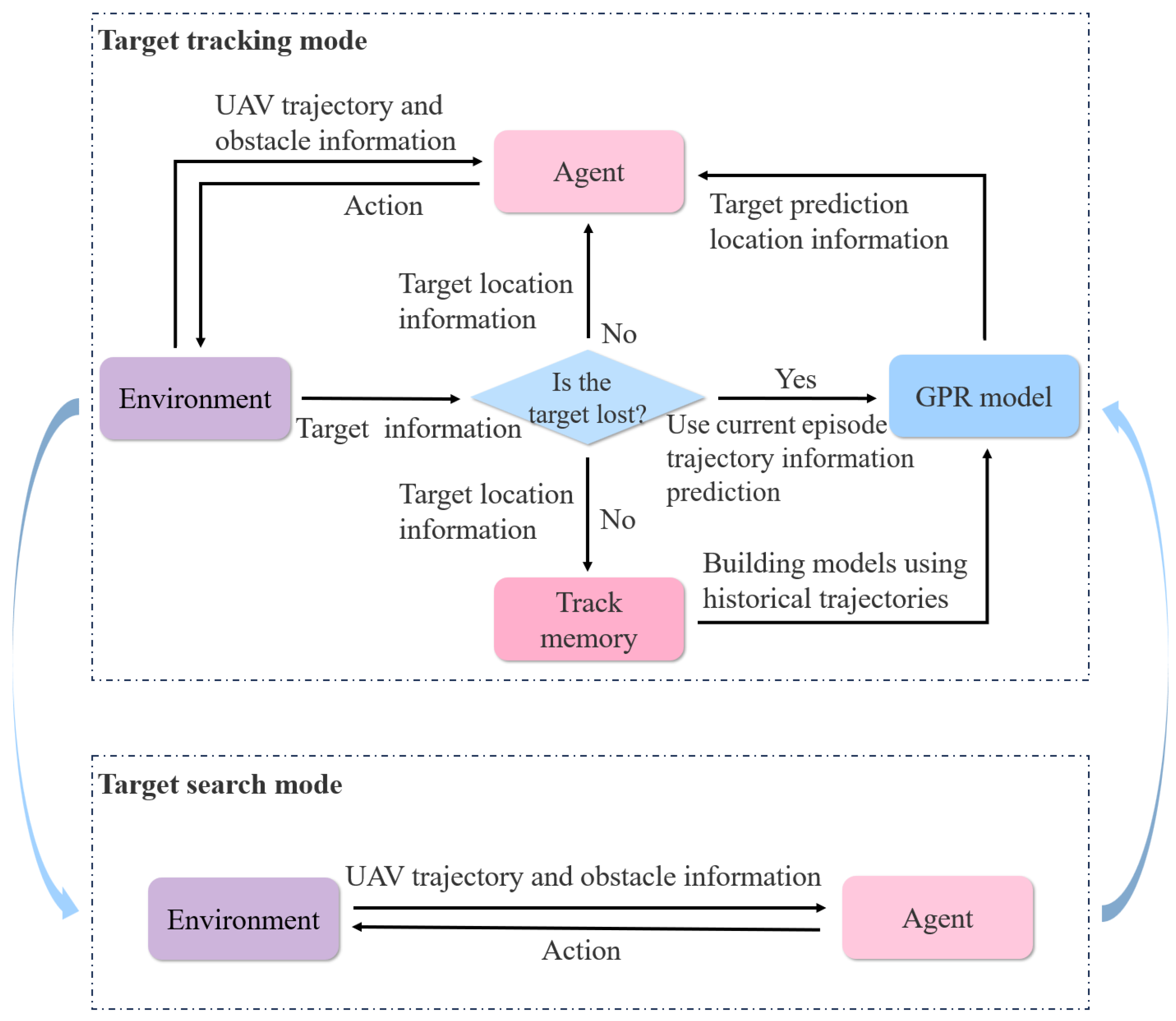
The incorporation of the target trajectory prediction method allows the UAV to quickly re-search and re-locate the target after temporarily losing the target position information. The system framework with the trajectory prediction method is shown in Figure 2, with the system operating in two modes: search mode and tracking mode. When the UAV detects the target, the system transitions from search mode to tracking mode. In tracking mode, if the target is lost, the agent treats the predicted target position as the true position and continues decision making. If the model’s predicted variance exceeds the set threshold, or if the number of predicted time steps reaches the set maximum prediction length $m_{max}$ and the target is still not found, the target is considered fully lost, and the system switches back to search mode.

3.4. Reward Function Design

RL uses rewards to estimate the expected return and derive the optimal policy. The design of the reward function is closely tied to the quality of the training outcome. A suitable reward function can accelerate training convergence and better guide the agent to perform favorable actions while avoiding undesirable ones. In the UAV target search and tracking problem, the reward design focuses on three key aspects: minimizing environmental uncertainty, find the target as quickly as possible, and maintaining tracking once the target is found. The entire search and tracking process should avoid collisions with threats. Based on these objectives, the reward function is defined as:

• Search Reward
  The objective of this reward function is to leverage spatial information entropy to encourage the UAV to explore uncovered areas and guide it in target search. Denote $k_1$ as the search reward coefficient, then the search reward is expressed as:

  $$r_{1,t}=k_1(H_{SI}^t-H_{SI}^{t-1})$$

  (26)
• Target Tracking Reward
  This reward function provides continuous rewards when the target is within the UAV’s FOV, guiding the UAV to keep tracking the target. Let $k_2$ represent the target tracking reward coefficient, then the target tracking reward function is defined as:

  $$r_{2,t}=\left\{\begin{array}{cc}{k}_2,\hfill & \mathrm{if}{P}_g^t\in \mathbb{Z}\hfill \\ 0,\hfill & \mathrm{otherwise}\hfill \end{array}\right.$$

  (27)
• Target Loss Penalty
  The purpose of this penalty function is to prevent the UAV from losing track of the target. Denote $k_3$ as the target loss penalty coefficient, then the target loss penalty is defined as:

  $$r_{3,t}=\left\{\begin{array}{cc}-k_3,\hfill & \mathrm{if}{P}_g^t\notin \mathbb{Z}\mathrm{and}{P}_g^{t-1}\in \mathbb{Z}\hfill \\ 0,\hfill & \mathrm{otherwise}\hfill \end{array}\right.$$

  (28)
• Collision Penalty
  This penalty function guides the UAV to avoid threats. Denote $k_4$ as the collision penalty coefficient, then the collision penalty is defined as:

  $$r_{4,t}=\left\{\begin{array}{cc}-k_4,\hfill & \mathrm{if}{P}_u^t\in \mathbb{B}\hfill \\ 0,\hfill & \mathrm{otherwise}\hfill \end{array}\right.$$

  (29)

The four rewards mentioned above work in unison, balancing the relationship between search, tracking, target loss, and collision risk via the reward function weights, offering a unified decision-making framework for the UAV. The weights of the reward function are set as hyperparameters. Initially, we made preliminary estimations of the importance of each reward component based on the experience of domain experts to set the initial weights. Subsequently, these hyperparameters were finely tuned through simulation experiments to balance the weights of different reward components, enabling the reward function to guide UAV action more effectively in complex environments. In summary, the complete reward function can be defined as:

$$r_t=r_{1,t}+r_{2,t}+r_{3,t}+r_{4,t}$$

(30)

3.5. Training Algorithm

RL tends to perform poorly in sample efficiency, especially when the UAV is tasked with search and tracking in complex dynamic environments. The RL agent typically needs extensive exploration and trial-and-error to gradually improve its decision-making abilities. However, conducting such extensive exploration in a real environment can lead to serious negative consequences. On one hand, the UAV may frequently collide during task execution, resulting in equipment damage or even property loss. On the other hand, this inefficient training method severely limits its applicability in high-risk, complex scenarios. Therefore, to enhance training efficiency and minimize potential risks in practical applications, this paper introduces the KbDDPG algorithm, which aims to accelerate RL convergence by using prior policy embedding in the policy network of the KANs structure.

KANs are inspired by the Kolmogorov–Arnold representation theorem, which states that any multivariate continuous function can be decomposed into a finite combination of univariate functions and addition operations. More specifically, for a smooth function $f:{[0,1]}^n\to R$:

$$f\left(x\right)=f(x_1,\cdots ,x_n)=\sum _{q=1}^{2n+1}{\mathsf{\Phi }}_q\left(\sum _{p=1}^n{\varphi }_{q,p}\left(x_p\right)\right)$$

(31)

where ${\varphi }_{q:p}:\left[0,1\right]\to \mathbb{R}$,${\mathsf{\Phi }}_q:\mathbb{R}\to \mathbb{R}$.

KANs parameterize each one-dimensional function in Expression (31) using B-spline curves. A KANs layer with $n_{in}$-dimensional input and $n_{out}$-dimensional output can be defined as a univariate function matrix:

$$\mathsf{\Phi }=\left\{{\varphi }_{q,p}\right\},p=1,2,\cdots ,n_{in},q=1,2\cdots ,n_{out}$$

(32)

where the function ${\phi }_{q,p}$ has trainable parameters.

Expression (31) can be represented as a simple combination of two KANs layers. However, KANs are not restricted to this structure. Similar to multi-layer perceptrons (MLPs), KANs can also expand the width and depth of their network. Given an input vector x, the output of KANs is:

$$KAN\left(x\right)=({\mathsf{\Phi }}_{L-1}\circ {\mathsf{\Phi }}_{L-2}\circ \cdots \circ {\mathsf{\Phi }}_1\circ {\mathsf{\Phi }}_0)x$$

(33)

All operations in the process are differentiable, allowing us to train KANs via backpropagation.

Traditional MLPs use fixed activation functions at the nodes, while KANs employ learnable activation functions at the edges. Each activation function in KANs is a univariate function parameterized by a spline curve, further improving the ability to approximate complex functions. These characteristics of KANs make their structure more intuitive and interpretable. The activation functions of KANs can be visually represented by spline curves, allowing researchers to interact with the model during simplification and optimization to modify or constrain certain function forms.

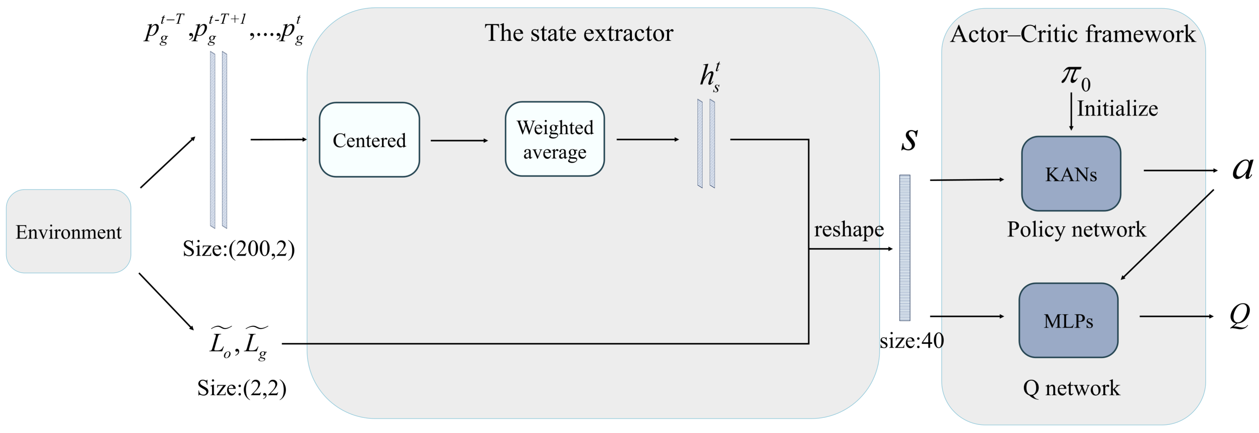
The structure of the KbDDPG algorithm is shown in the Figure 3. $f_s$ is used to process the UAV trajectory data. First, the data is centralized to standardize the input, improving the robustness of the state representation and enhancing generalization ability. Then, a weighted average is applied to compress the data length and increase information efficiency. Finally, the processed data is combined with the target and obstacle position information, serving as the agent’s state input. Additionally, in the traditional deep deterministic policy gradient (DDPG) algorithm, the policy network determines the action to take given a state, while the value network estimates the $Q^{\pi }(s,a)$ for the current state–action pair. Both the policy network and the value network typically use MLPs structure [32]. KbDDPG modifies the policy network by replacing the original MLPs structure with a KANs structure that includes prior policy, while the value network retains its MLPs architecture.

We assume that researchers can design a simple, low-performance prior policy ${\pi }_0\left(s\right)$ in advance, based on the agent’s state and environmental information. The prior policy helps the agent explore the environment and achieve its objectives. Due to the structural properties of KANs, the activation functions can be set to known symbolic forms, enabling the model to represent traditional mathematical expressions. 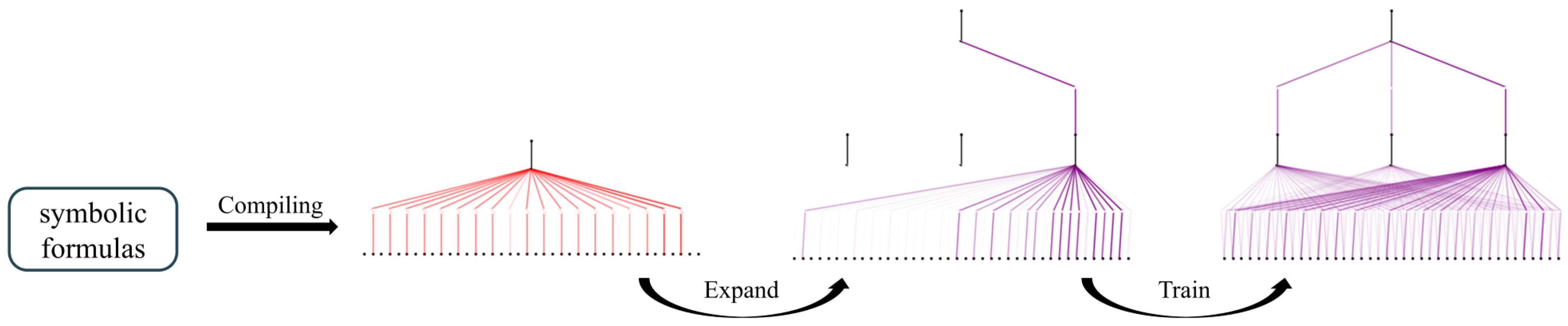In RL, we can embed an existing prior policy ${\pi }_0\left(s\right)$, which is represented symbolically, into a trainable KANs, resulting in a KANs that incorporates initial policy [33]. This process involves three main steps, as shown in Figure 4:

• Compile symbolic formulas into KANs: First, parse the symbolic formulas into a tree structure, where nodes represent expressions and edges represent operations/functions. Then, modify the tree to align it with the KANs structure. This modification involves moving all leaf nodes to the input layer via virtual edges and adding virtual sub-nodes/nodes to match the KANs architecture. These virtual edges/nodes/sub-nodes perform only transformations. Finally, the variables are combined at the first layer, effectively converting the tree into a graph.
• Extend the network: The compiled KANs network structure is compact, without redundant edges, which could limit its expressive power and hinder further fine-tuning. To improve expressiveness, the network width and depth can be increased according to the task complexity.
• Training: The agent, after policy initialization, already possesses a certain ability to complete tasks, which can significantly accelerate the convergence speed of subsequent training and reduce the task failure rate during the training process. Finally, building on the prior policy, the strategy is further optimized using DRL algorithms.

The policy network ${\pi }_{KAN}(s_t,{\theta }_{KAN})$, which embeds the prior policy ${\pi }_0\left(s\right)$, is used to generate the action based on the current state $s_t$:

$$a_t={\pi }_{KAN}(s_t;{\theta }_{\pi })$$

(34)

By executing the action $a_t$, interacting with the environment, and receiving the next state $s_{t+1}$, reward $r_t$, and done flag, the current experience $(s_t,a_t,r_t,s_{t+1})$ is obtained and stored in the experience replay buffer $\mathcal{D}$. The value network and policy network are updated by randomly sampling experience data $B={\left\{(s_i,a_i,r_i,s_{i+1})\right\}}_{i=1}^N$ from the experience replay buffer. According to Equation (14), the target Q-value is expressed as:

$$y_i=r_i+\gamma Q^{\prime }(s_{i+1},{{\pi }^{\prime }}_{KAN}(s_{i+1};{\theta }_{\pi }^{\prime });{\theta }_Q^{\prime })$$

(35)

where $y_i$ is the target value of the i-th experience data, $Q^{\prime }$ and ${{\pi }^{\prime }}_{KAN}$ represent the target network, which is specifically used to compute the target value.

During training, to make the target network updates smoother, it uses soft updating to gradually approach the value network and policy network, with the soft update coefficient $\tau$ controlling the target network parameter update speed. The objective of the value network is to approximate the true Q-values by minimizing the mean squared error (MSE) loss of the Q-value function. Thus, the loss function for the value network is defined as the MSE between the predicted Q-values and the target Q-values:

$$L_Q\left({\theta }_Q\right)={\displaystyle \frac{1}{N}}\sum _{i=1}^N(y_i-Q(s_i,a_i;{\theta }_Q){)}^2$$

(36)

The gradient of the value network is the derivative of the loss function with respect to the parameter ${\theta }_q$:

$${\nabla }_{{\theta }_Q}{L}_Q\left({\theta }_Q\right)={\displaystyle \frac{2}{N}}\sum _{i=1}^N\left(Q(s_i,a_i;{\theta }_Q)-y_i\right){\nabla }_{{\theta }_Q}Q(s_i,a_i;{\theta }_Q)$$

(37)

The objective of the policy network is to find the optimal policy by maximizing the Q-value output by the value network. The goal is to maximize the expected return under the policy. The loss function of the policy network can be defined as the negative Q-value:

$$L_{\pi }\left({\theta }_{\pi }\right)=-{\displaystyle \frac{1}{N}}\sum _{i=1}^{N}Q(s_i,{\pi }_{KAN}(s_i;{\theta }_{\pi });{\theta }_Q)$$

(38)

Since the policy network embeds prior policy ${\pi }_0$, the policy network can be represented as:

$$\pi (s;{\theta }_{\pi })={\pi }_0\left(s\right)+\Delta \pi (s;{\theta }_{\pi })$$

(39)

where $\Delta \pi (s;{\theta }_{\pi })$ represents the difference between the current network and the prior policy.

At the beginning of training, the network difference is zero. This way, the network has a reasonable behavioral foundation from the start. Compared to traditional reinforcement learning algorithms, this effectively reduces the inefficiency caused by starting exploration from a completely random policy. Additionally, in terms of network training, the derivative of the policy network with respect to the parameters can be expressed as:

$${\nabla }_{{\theta }_{\pi }}{L}_{\pi }\left({\theta }_{\pi }\right)=-{\displaystyle \frac{1}{N}}\sum _{i=1}^N{\nabla }_{a}Q(s_i,a;{\theta }_Q){|}_{a={\pi }_0\left(s\right)+\Delta \pi (s;{\theta }_{\pi })}{\nabla }_{{\theta }_{\pi }}\Delta \pi (s;{\theta }_{\pi })$$

(40)

It can be observed that the gradient in the above equation only involves the $\Delta \pi (s;{\theta }_{\pi })$ part, meaning that the network only needs to learn the correction term of the ideal policy relative to the prior policy. At the same time, the prior policy ${\pi }_0$ provides a starting point close to the optimal solution, reducing the exploration range and making the gradient direction more stable, which significantly reduces the complexity of the learning task and accelerates convergence. Parameters are updated using gradient descent in the direction opposite to the gradient:

$$\left\{\begin{array}{c}{\theta }_Q\leftarrow {\theta }_Q-l_c{\nabla }_{{\theta }_Q}{L}_Q\left({\theta }_Q\right)\hfill \\ {\theta }_{\pi }\leftarrow {\theta }_{\pi }-l_a{\nabla }_{{\theta }_{\pi }}{L}_{\pi }\left({\theta }_{\pi }\right)\hfill \end{array}\right.$$

(41)

where $l_c$ and $l_a$ are the learning rates for the policy network and value network, respectively.

As learning progresses, the policy network is continuously optimized, and the agent gradually moves away from the prior policy’s influence, independently achieving the task objectives. In summary, the proposed algorithm can be summarized as Algorithm 1.

Algorithm 1 KbDDPG Algorithm

1: Randomly initialize critic network $Q(s,a|{\theta }_Q)$ with weights ${\theta }_Q$ 2: Compile the initial policy ${\pi }_0\left(s\right)$ into ${\pi }_{KAN}(s_t,{\theta }_{KAN})$ 3: Extend the KANs ${\pi }_{KAN}(s_t,{\theta }_{KAN})$ 4: Initialize target network $Q^{\prime }$ and ${\pi }_{KAN}^{\prime }$ with weight ${\theta }_Q^{\prime }\leftarrow {\theta }_Q,{\theta }_{\pi }^{\prime }\leftarrow {\theta }_{\pi }$ 5: Initialize replay buffer R 6: for each episode = 1,M do 7:    Initialize a random $\mathcal{N}$ process for action exploration 8:    Receive initial observation state $s_1$ 9:    for each episode = 1,T do 10:      Select the action $a_t=\pi (s_t|{\theta }_{KAN})+{\mathcal{N}}_t$, ${\mathcal{N}}_t$ represents the exploration noise 11:      Execute action $a_t$ and observe reward $r_t$ and observe new state $s_{t+1}$ 12:      Store transition $(s_t,a_t,r_t,s_{t+1})$ in R 13:      Sample a random minibatch of transitions $(s_t,a_t,r_t,s_{t+1})$ from R 14:      Set $y_i=r_i+\gamma Q^{\prime }(s_{i+1},{{\pi }^{\prime }}_{KAN}(s_{i+1};{\theta }_{\pi }^{\prime });{\theta }_Q^{\prime })$ 15:      Update critic by minimizing the loss: $$\begin{array}{l}{\nabla }_{{\theta }_Q}{L}_Q\left({\theta }_Q\right)={\displaystyle \frac{2}{N}}{\displaystyle \sum _{i=1}^N}\left(Q(s_i,a_i;{\theta }_Q)-y_i\right){\nabla }_{{\theta }_Q}Q(s_i,a_i;{\theta }_Q)\hfill \\ {\theta }_Q\leftarrow {\theta }_Q-l_c{\nabla }_{{\theta }_Q}{L}_Q\left({\theta }_Q\right)\end{array}$$ 16:      Update the actor policy using the sampled policy gradient: $$\begin{array}{l}{\nabla }_{{\theta }_{\pi }}J={\displaystyle \frac{1}{N}}{\displaystyle \sum _i}{\nabla }_{a}Q(s,a|{\theta }_Q){|}_{s=s_i,a=\pi \left(s_i\right)}{\nabla }_{{\theta }_{\pi }}\pi (s|{\theta }_{\pi }){|}_{s_i}\hfill \\ {\theta }_{\pi }\leftarrow {\theta }_{\pi }-l_a{\nabla }_{{\theta }_{\pi }}{L}_{\pi }\left({\theta }_{\pi }\right)\hfill \end{array}$$ 17:      Update the target networks: $$\begin{array}{c}{\theta }_Q^{\prime }\leftarrow \tau {\theta }_Q+(1-\tau ){\theta }_Q^{\prime }\hfill \\ {\theta }_{\pi }^{\prime }\leftarrow \tau {\theta }_{\pi }+(1-\tau ){\theta }_{\pi }^{\prime }\hfill \end{array}$$ 18:    end for 19: end for

4. Experiments

This section evaluates the performance of the model and algorithm through several experiments. First, we describe the simulation environment and experimental parameters. Next, we compare the success rate of relocating the target before and after using target trajectory prediction, and visualizing the prediction results. We then analyze the impact of spatial information entropy on target search and compare the search performance with other baseline algorithms. Lastly, we compare the proposed KbDDPG algorithm with other baseline methods and visualize the UAV task execution to assess its convergence performance.

4.1. Simulation Environment Design

To verify the adaptability of the UAV system in complex environments, we built a highly complex virtual environment through simulation. These environments feature a large number of irregularly distributed static obstacles, and also simulate tracking targets that move dynamically with random starting positions. In addition, multiple occlusion areas were set in the test environment to simulate potential sensor blind spots and noise interference in real-world scenarios. The UAVs can only acquire environmental and target information within a limited range. This limitation further intensifies the uncertainty and dynamics of the environment, while also requiring the system to fully consider the coverage and redundancy of information acquisition when planning search paths. The randomness and dynamic changes in various factors in the environment make the entire scene much more complex than traditional static or single-obstacle environments, fully testing the UAV’s robustness and flexibility in tasks such as searching, continuous tracking, and rapid re-localization after target loss.

The virtual environment uses polygonal areas to represent obstacles and line-of-sight occlusion zones. If the UAV collides with an obstacle, the task is considered failed, and the UAV cannot detect targets entering the line-of-sight occlusion zones. The environment is stochastic, with the UAV’s starting position and target position being randomly re-initialized at the end of each navigation task. For the KbDDPG algorithm, we design a simple initial control policy ${\omega }_u^t={\varphi }_g^t-k_p{\varphi }_o^t$, where the coefficient $k_p$ is used to balance the weights between UAV tracking and obstacle avoidance. In the simulation, the target trajectory information from the most recent 50 episodes is stored for trajectory prediction. The UAV’s historical trajectory is recorded for up to 100 steps and processed by a state extractor to generate a state input of length 40. After embedding the prior policy, 2 additional KANs nodes are added to the policy network. The value network has 512 hidden layer nodes. The simulation experiments in this paper were conducted in a Windows 11 environment using Python 3.11 and Pytorch 2.2.1. Gaussian process regression was implemented based on Scikit-learn 1.4.2, and the KAN network was constructed using Pykan 0.2.6. The simulation environment was built following the OpenAI Gym API standards. The experiments were run on a computer equipped with i7-11700F CPU, RTX 3060 GPU (12 GB VRAM), and 16 GB of RAM. The reinforcement learning training used the Adam optimizer, and 3300 s were needed to complete 100 training episodes. Other parameters of the virtual simulation environment are shown in

Table 1. Simulation parameters.

Parameter	Description	Value
M	Simulation environment size	125
${\omega }_n$	UAV angular velocity range	[−1, +1]
v	UAV velocity	3
R	UAV maximum perception range	12
$\gamma$	Discount factor	0.99
$\alpha$	Decay coefficient	0.015
$T_{max}$	Maximum number of steps	500
$w_{max}$	Prediction model input length	30
$m_{max}$	Prediction length	20
d	Increment value for the window	4
u	Number of window uses	3
$k_1$	Search reward coefficient	200
$k_2$	Tracking reward coefficient	5
$k_3$	Target loss penalty coefficient	25
$k_4$	Collision penalty coefficient	200
$l_a$	Policy network learning rate	$5\times {10}^{-4}$
$l_c$	Value network learning rate	$2\times {10}^{-3}$
$\beta$	Adam optimizer hyperparameters	(0.9, 0.999)
$\tau$	The rate of soft update	$5\times {10}^{-3}$
$k_p$	Avoidance coefficient	10

. Unless otherwise specified, the parameters in the table are used for the simulation.

4.2. Performance Analysis of the Prediction Model

We tested the trajectory prediction performance of the proposed GPR model, which inputs data from 20 time steps and outputs 10 predicted values. Figure 5 displays the prediction results for both straight-line and turning motion when the target enters the line-of-sight occlusion zone. We observed that GPR provides accurate fitting after the target is lost. Additionally, the probability distribution generated by GPR quantifies the uncertainty in the estimates. We can see that as the prediction time steps increase, the uncertainty of the prediction gradually grows, which helps in evaluating the quality of the prediction.

Table 2. Model prediction performance.

Number of Samples	Success Rate	Mean Error
0	0.197	-
50	0.901	3.765
100	0.929	3.485
500	0.935	3.480
1000	0.935	3.479
1500	0.937	3.470

presents the prediction performance when the target enters the line-of-sight occlusion zone in UAV tracking mode. For each prediction, if the target remains within the UAV’s FOV after exiting the line-of-sight occlusion zone, the prediction is deemed successful. It is clear that, compared to no prediction (sample size of 0), our prediction model significantly improves the UAV’s success rate in locating the lost target. As the number of model samples increases, its performance improves, but the increase is marginal, suggesting that the model performs well with small datasets and does not require a large amount of training data.

4.3. Search Performance Analysis

In this section, we test the effect of different parameters $\alpha$ on search performance. Furthermore, to validate the performance of our method, we compare the proposed RL-based search strategy with the complete coverage path planning and random walk methods. The coverage path planning method divides the workspace into sub-regions and explores them using simple back-and-forth motion, achieving complete area coverage. The random walk method is based on the concept of random motion. The UAV maintains straight flight when no obstacles are detected. Once an obstacle is detected ahead, the UAV randomly samples an angle change value to determine a new flight direction. After adjusting its direction, the UAV resumes straight flight and repeats the process [34].

Figure 6 visualizes the information correlation density. The heatmap illustrates how the spatial information correlation density changes over time steps for different $\alpha$ values, given the same UAV trajectory. On the horizontal axis, as the time steps increase, the information correlation density uniformly distributed across the environment decreases, while the correlation density in the explored regions increases, indicating that the UAV perceives these areas as having lower information search efficiency. On the vertical axis, when $\alpha$ is small, the information relevance density changes slowly. Information updates are not timely, and the differences in information density between regions are small. Although the historical positions of the UAV influence information relevance density for a longer time, excessively old historical information may interfere with the search for moving targets. As $\alpha$ increases, the spatial information density changes more dramatically with the UAV’s movement. However, the rapid rate of change also causes the information relevance density at historical positions to decline rapidly, leading to a loss of historical exploration information.

We define environmental coverage as the ratio of the number of coordinates covered by the UAV’s FOV during an episode to the total number of coordinates that can be explored in the environment. The parameter $\alpha$ controls the decay rate of the spatial information density, thus influencing search performance. To determine the optimal $\alpha$ value, we tested the impact of RL strategies trained with different $\alpha$ values on the UAV’s environmental exploration rate, as shown in Figure 7. When the parameter value is small, the coverage performance is relatively poor, with high variance. As the parameter value increases, the environmental coverage gradually rises, reaching its peak near $\alpha =0.015$. Indicating more stable and effective search performance within this range. As $\alpha$ continues to increase, coverage begins to decline, indicating that both very small and very large $\alpha$ values lead to decreased coverage. This is also consistent with our earlier discussion on information correlation density.

Figure 8 presents the comparison results of the search algorithm at different target speeds for $\alpha =0.015$. From the figure, we can observe that as the target speed increases, the success rate of the coverage path planning method gradually decreases from 1.0, reaching its worst performance at medium target speeds. This suggests that coverage path planning, which relies on a fixed path for complete coverage, works well for stationary and low-speed targets, leveraging the advantage of spatial coverage. However, at medium speeds, the probability of missing the target increases, and due to its inflexibility, it becomes challenging to relocate the target after missing it in the first scan of each coverage cycle. Random walk shows a low success rate at low target speeds. As the target speed increases, the success rate gradually improves, but its overall performance is inferior to that of the other two algorithms. Our method shows stable and efficient search performance at all speeds, especially at medium target speeds, where it significantly outperforms the other two methods. Additionally, at higher target speeds, the success rates of the three algorithms are similar, and all algorithms perform well in completing the search task. This suggests that under high-speed conditions, the performance differences between the algorithms are minimal, with target speed being the dominant factor rather than the specific algorithm design.

Figure 9 displays the motion trajectories of 1000 targets. We can observe that, influenced by the control method and obstacles, the probability of target appearance differs at various locations. We believe that RL-based methods offer greater robustness, as they can learn to capture the target’s hidden behavior patterns and exhibit strong adaptability to targets with different behaviors. Figure 10 presents the relationship between time steps and search success rate for the three search algorithms within a single episode. From the figure, we can see that our method shows a higher search success rate in most cases.

4.4. Convergence Performance Analysis

Next, we compare DDPG, DDPG from demonstrations (DDPGfD), KAN-DDPG, and KbDDPG, training each algorithm for 100 episodes in the same environment to collect our experimental data. DDPGfD is an algorithm that combines expert demonstration data with DRL. It is an improvement on the DDPG algorithm that accelerates the learning process by incorporating expert demonstration data. In this experiment, we use an agent trained with DDPG to interact with the environment and collect demonstration data. KAN-DDPG replaces the policy network of the DDPG algorithm with KANs, maintaining the same network structure as our algorithm but without without prior policy embedding. Figure 11 shows the reward progression for each episode during training. It can be observed that KbDDPG converges faster than both DDPG and KAN-DDPG. Although DDPGfD converges very quickly, its convergence starts later than our algorithm. This indicates that the KbDDPG algorithm demonstrates strong performance from the early stages of training. The results demonstrate that the KbDDPG algorithm leverages prior policy to efficiently learn critical information from the environment in the initial stages, leading to faster reward improvement.

Figure 12 presents the collision rate and target tracking duration during the training process. The collision rate is defined as the ratio of episodes where the UAV collides to the total number of experiments, which we use to evaluate the UAV’s obstacle avoidance ability. Target tracking duration is defined as the number of time steps the target remains within the UAV’s field of view during each episode. We use it to evaluate the UAV’s target search and tracking capability. As shown in Figure 12a, the other algorithms start with a collision rate of 1 and require multiple trial-and-error collisions to converge. In contrast, KbDDPG maintains a collision rate of about 0.4 from the start of training. As training progresses, the collision rate decreases further and stabilizes near 0, which is crucial for reducing equipment wear during real-world training. As shown in Figure 12b, our algorithm maintains around 50 target tracking duration steps at the beginning of training, and stabilizes at about 300 as training progresses. The results in Figure 12 show that KbDDPG has obstacle avoidance and target search and tracking abilities from the start of training, meaning that the algorithm successfully embeds the prior policy into the policy network. Meanwhile, we have observed that the performance of the KAN-DDPG algorithm consistently ranks the lowest. We attribute this to the fact that while the KAN structure enhances the network’s expressive power by learning activation functions, it also complicates the optimization problem. Without a prior policy to serve as a “good starting point” to guide the network’s learning, the optimization space becomes larger and harder to explore, making it difficult for the network to quickly converge to an effective policy.

To further assess the algorithm’s performance after training convergence, we conducted task performance tests. Figure 13 shows the results of the trained reinforcement learning agent performing target search and tracking in different environments, with 300 time steps tested for each environment. As illustrated in the figure, during the search phase, the UAV conducts a broad search across the area, exploring potential target locations in the environment. In the tracking phase, the UAV is able to stably track the target, successfully avoid obstacles, and mitigate interference from occluded regions. Meanwhile, the UAV is unaffected by changes in obstacle distribution and can consistently complete the task under various obstacle layouts. Figure 14 displays the results of the agent’s target search and tracking in environments of different sizes, expanding the task to larger, more complex obstacle settings. The 200-grid and 300-grid sizes environments were tested for 500 and 700 time steps, respectively, while other environments were tested for 300 time steps. It can be seen that regardless of the scene size, the trained agent exhibits excellent search and tracking performance. In smaller environments, the agent swiftly covers the entire area, quickly locating and locking onto the target. In larger, more complex environments with a broader target activity range, the agent effectively expands its search to locate the target. The results indicate that the trained agent performs well in target search and tracking tasks, demonstrating strong adaptability and robustness in different environments.

5. Discussion

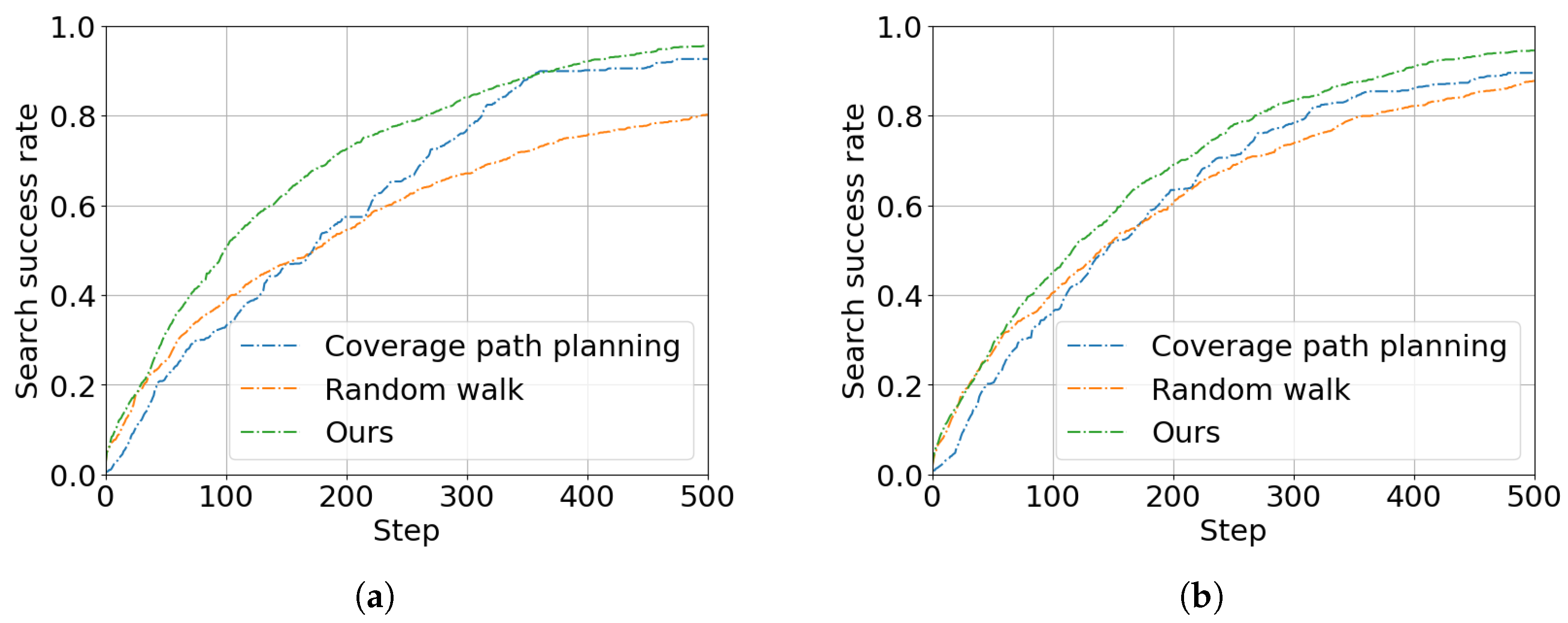
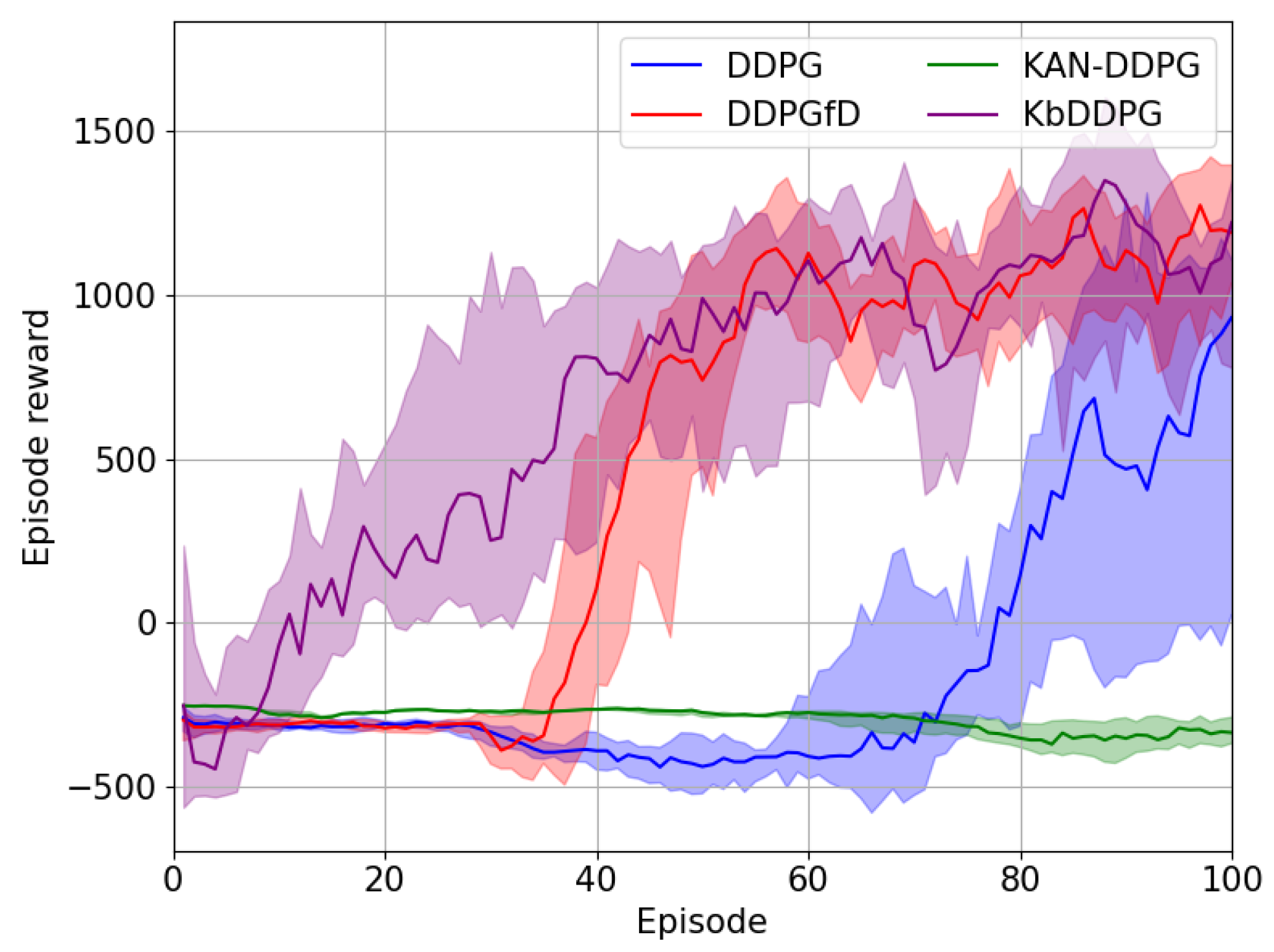
In this paper, we focus on the UAV target search and tracking problem. We use the GPR model to predict the target’s trajectory, addressing the target loss issue. Furthermore, we extend the concept of spatial information entropy to target search. To address the issue of low sample efficiency in DRL, we propose a novel DRL algorithm based on KANs. A large number of simulation results demonstrate that, compared to other DRL algorithms, our method shows superior convergence performance. Moreover, due to the application of spatial information entropy, our method outperforms existing path planning algorithms in target search.

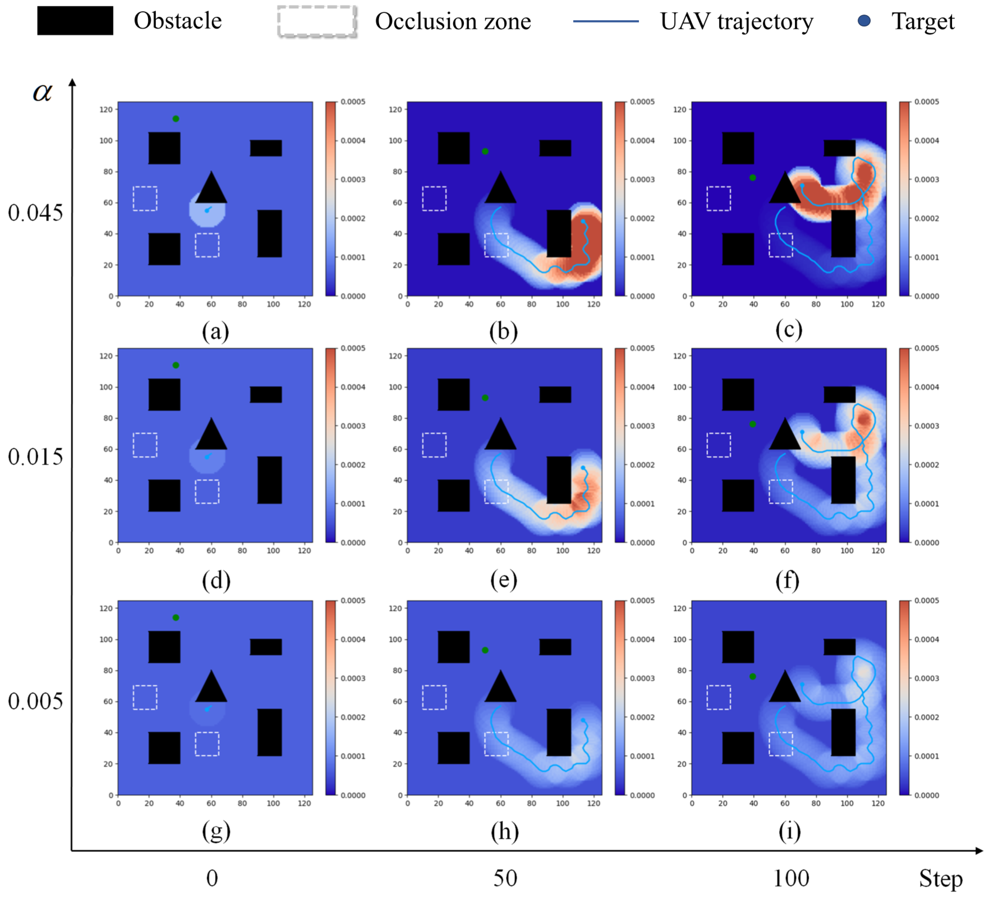
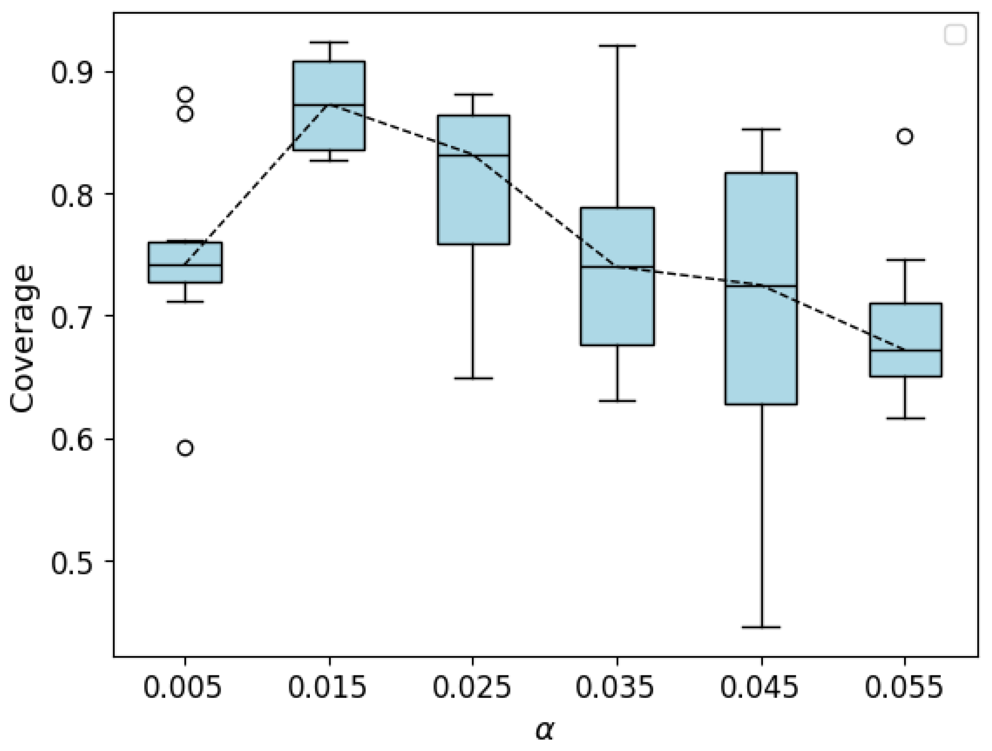
However, in the simulation, we made the simple assumption that the target’s next state only depends on the current state. In reality, the target’s movement contains higher-order dependencies, its behavior is more unpredictable, and it may even exhibit evasive actions against the searching UAV. Therefore, more reasonable modeling of the target’s movement will be a direction for our future research. Additionally, our study on the information correlation density decay coefficient alpha is limited to the optimal value in the same environment. However, the decay coefficient can be designed to adjust adaptively according to the environment. Thus, our future work will consider introducing an adaptive adjustment mechanism to enhance the flexibility and robustness of the algorithm in different dynamic environments. Meanwhile, although our virtual environment design considers factors such as obstacles, occlusion zones, and target movement, to simplify the study and improve computational efficiency, we still adopted simplified modeling for UAV dynamics, sensor noise, and target behavior, and restricted the environment to a 2D space. In real environments, UAV flight dynamics are often more complex, with various random noises bringing additional interference to the UAV’s decision making. There is often a performance gap between the simulation environment and real-world applications. We have not yet conducted comprehensive tests on real UAV platforms, and we plan to explore the deployment of DRL algorithms on real UAVs in future work, further improving the method to address more non-ideal factors in real environments. Finally, this paper only verifies the impact of relatively simple prior policies on the algorithm. In future work, we will delve deeper into the reinforcement learning algorithm based on KANs to explore its potential in complex tasks and further improve the algorithm’s performance in high-dimensional continuous action spaces.