Precise Position Estimation of Road Users by Extracting Object-Specific Key Points for Embedded Edge Cameras

Abstract

Detecting road users and estimating accurate positions are significant in intelligent transportation systems (ITS). Most monocular camera-based systems for this purpose use 2D bounding box detectors to obtain real-time operability. However, this approach has the drawback of causing large positioning errors due to the use of upright rectangles for every type of object. To overcome this shortcoming, this paper proposes a method that improves the positioning accuracy of road users by modifying a conventional 2D bounding box detector to extract one or two additional object-specific key points. Since these key points are where the road users contact the ground plane, their accurate positions can be estimated based on the relation between the ground plane on the image and that on the map. The proposed method handles four types of road users: cars, pedestrians, cyclists (including motorcyclists), and e-scooter riders. This method is easy to implement by only adding extra heads to the conventional object detector and improves the positioning accuracy with a negligible amount of additional computational cost. In experiments, the proposed method was evaluated under various practical situations and showed a 66.5% improvement in road user position estimation. Furthermore, this method was simplified based on channel pruning and embedded on the edge camera with a Qualcomm QCS 610 System on Chip (SoC) to show its real-time capability.

1. Introduction

Research on detecting road users and estimating their positions is significantly important in intelligent transportation systems (ITS). For instance, vehicle-to-infrastructure (V2I)-based autonomous driving, one of the key ITS applications, relies on perception sensors mounted on infrastructures to acquire the positions of road users. Autonomous vehicles utilize this information for safe navigation or collision avoidance [1,2].

Monocular cameras are undoubtedly one of the most widely used sensors in ITS applications. Road user detection methods using monocular cameras can be mainly categorized into two approaches according to how they represent objects: 3D bounding box-based and 2D bounding box-based. The 3D bounding box-based approach can enhance the performance of traffic analysis and the safety of autonomous driving by providing more information on road users. However, it has some drawbacks in terms of monocular camera-based real-time edge processing. First, its performance is limited because extracting 3D information from a 2D image is significantly challenging. This is why practical applications utilize Lidar-camera fusion [3,4]. Second, due to its high difficulty level, it should utilize a heavy and complex network [5,6]. This makes it challenging to embed into edge devices and run in real time. These are the main reasons many practical real-time camera-based applications still use the 2D bounding box-based approach.

The 2D bounding box-based approach usually estimates a road user’s position by calculating a specific location based on the detected bounding box and projecting it onto the ground plane of the map [7,8,9,10]. The most common method is to use the center or bottom center of the detected bounding box. Although this method can be easily implemented in practical applications, it inevitably produces position errors. Figure 1a shows the position error when using the center of the bounding box. In this figure, the black cross and black dot indicate the center of the bounding box and the corresponding position on the ground, and the red dot indicates the actual position of the detected car. It can be clearly noticed that a significant error exists between the actual (red dot) and estimated (black dot) positions. Figure 1b shows the position error when using the bottom center of the bounding box. In this figure, the black cross and black dot indicate the bottom center of the bounding box and the corresponding position on the ground, and the red dot indicates the actual position of the detected motorcyclist. This case also shows a significant error between the actual (red dot) and estimated (black dot) positions.

To overcome the drawbacks of the 2D bounding box-based approach, this paper proposes two methods to precisely estimate the positions of various road users using a monocular surveillance camera. The two proposed methods detect four types of road users: cars, pedestrians, cyclists (including motorcyclists), and e-scooter riders. The first proposed method detects one imaged location of the road user’s bottom face center in world coordinates along with its bounding box. This method is called a one-point detector in this paper. Red dots in Figure 2a indicate the bottom face centers of the road users in world coordinates, while red dots in Figure 2b show their imaged locations. If the red dots in Figure 2b are detected in images, their positions in world coordinates can be more precisely estimated compared to the center or bottom center of the bounding box. The proposed method directly extracts this location for four types of road users, unlike previous methods, which indirectly extract this location [11,12] or restrict its use to cars only [10,13]. The second proposed method detects two imaged locations of the road user in world coordinates along with its bounding box. This method is called a two-point detector in this paper. The two locations are determined according to the type of road users, as shown in Figure 2a,c with blue and green dots (car: front and rear bottom centers, pedestrian: left and right feet, cyclist and e-scooter rider: bottom centers of two wheels). This two-point detector provides more information on road users than the one-point detector because their sizes, headings, and positions can be estimated based on the two points and the line segment connecting them.

This paper implements the proposed one-point and two-point detectors by adding extra heads to a popular CNN-based object detector (YOLO) instead of developing a new complex and heavy network architecture. In addition, the proposed detectors were simplified via channel pruning and embedded into an edge device with a Qualcomm QCS610 System on Chip (SoC) to confirm its real-time applicability. Since this paper shows that minimal modifications of the conventional object detector can improve ITS systems, many practitioners can easily reimplement and run it in real-time embedded edge devices. In experiments, the proposed methods were evaluated using images taken from 16 cameras at different sites. Evaluation results reveal that these methods significantly improve the positioning accuracy of road users by up to 66.5% and run at about 10 frames per second in the embedded edge device.

This paper is organized as follows: Section 2 introduces related research works. Section 3 explains the details of implementing the proposed methods. Section 4 presents the experimental results and analyses. Finally, this paper concludes with a summary and future work in Section 5.

2. Related Works

Since this paper suggests methods for precisely detecting the positions of road users, this literature review focuses on previous detection methods that enhance the positioning accuracy of road users, especially cars, pedestrians, cyclists (including motorcyclists), and e-scooter riders.

2.1. Car Detection

Existing car detection methods that provide precise positions include the car’s bottom face detection approach [14,15] and 3D bounding box detection approach [3,5,6,16,17,18,19,20,21,22,23,24]. These two approaches provide detection results that contain information on the car’s location, size, and direction. Ref. [14] performs homography estimation using satellite images from a public map service and detects the car’s bottom face from bird’s-eye view BEV images. Ref. [15] proposes three simple deep learning-based bottom face detection methods for cars: the corner-based approach, the position, size, and angle (PSA)-based approach, and the line-based approach. Ref. [3] creates a 3D bounding box by detecting the four vertices of the bottom face and the height from the ground. Ref. [16] extends the single-shot multibox detector (SSD) [25] and generates a 3D bounding box based on the detected 2D bounding box. Four vertices are used to create a 3D shape, of which three vertices are used for the bottom face of the car, and the remaining vertex is used to create the car height. Refs. [17,18,19,20] detect the 3D bounding box of the car by detecting a total of eight vertices. Ref. [17] estimates the distance between the center of the 2D bounding box and each vertex, and [18] estimates the distance between the bottom left corner of the 2D bounding box and each vertex to detect eight vertices. Refs. [19,20] create a heatmap similar to the CenterNet [26] and detect eight vertices based on the heatmap. Ref. [5] also detects eight vertices using a complex network composed of four subnetworks. Ref. [6] utilizes a model with two subnetworks. It detects 3D bounding boxes by predicting the position, dimension, and angle, instead of detecting vertices. Refs. [21,22,23,24] also predict the position, dimension, and angle to find bounding boxes. Refs. [21,22] generate a 3D bounding box by calculating the average size from the training dataset and combining it with the estimated position and rotation angle. Refs. [23,24] predict the rotation angle using the multi-bin method [27]. To find the position, ref. [23] uses the bottom face center of the bounding box and [24] uses the center of the bounding box.

2.2. Pedestrian Detection

Most existing methods detect pedestrians with 2D bounding boxes [28,29,30,31]. Among them, ref. [30] considers the pedestrian’s position as the bottom center of the 2D bounding box, and [31] considers it the center of the 2D bounding box. As explained in Figure 1, these methods inevitably generate position errors. A more precise location can be determined by applying human pose estimation techniques to the detected pedestrian 2D bounding box [32,33,34]. Ref. [32] proposes a symmetric spatial transformer network with a parallel single-person pose estimator to extract high-quality single-person regions and perform pose estimation. Ref. [33] uses Faster R-CNN with an additional branch to predict the 2D bounding box with its segmentation mask and predicts key points for pose estimation using a one-hot mask. Ref. [34] first detects 2D bounding boxes and estimates key points using a cascaded pyramid network (CPN) composed of two subnetworks. The CPN includes a global pyramid network that handles simple key points and a pyramid-refined network that handles hard key points. Various studies on detection in the form of 3D bounding boxes have also been conducted [6,24,35,36,37]. Ref. [36] utilizes two sets of regression head branches. The first set detects essential information such as position, size, and angle, and the second set detects auxiliary information such as the projected positions of the eight vertices and center of the 3D bounding box. Ref. [37] utilizes YOLOv3 to detect regions of interest (ROI) and generates a 3D bounding box by regressing parameters for size, distance, direction, and location in meters within the ROI. Ref. [24] detects a 3D bound box by employing prior knowledge of the object’s dimension and a 2D bounding box detected using YOLOv5. Ref. [6] produces a 3D bounding box using the pedestrian’s position, size, and angle predicted in the two subnetworks. Ref. [35] calculates the pixel-to-meter ratio using satellite images to convert a 2D bounding box into a 3D bounding box. Assuming that the bottom center of the detected 2D bounding box coincides with the bottom face center of the 3D bounding box, the bottom face size is calculated by applying the pixel-to-meter ratio to the approximate size given by prior knowledge. The 3D bounding box is then created using the empirically determined height ratio.

2.3. Cyclist (Motorcyclist) and E-Scooter Rider Detection

Cyclist and motorcyclist detection methods can also be categorized into a 2D bounding box-based approach [28,29,38,39] and a 3D bounding box-based approach [6,24,27,35,36,37]. Ref. [29] proposes a unified framework for detecting pedestrians and cyclists. This framework consists of three steps: upper body detection, generation of potential regions covering the whole instance, and classification and localization. Ref. [39] employs SSD to detect cyclists, while [38] uses Aggregated Channel Features [40], Deformable Part Models [41], and Fast R-CNN [42]. Ref. [43] handles only the scenario where a single cyclist is in the image. It uses a part-based feature produced by combining appearance-based and edge-based features. The appearance-based feature consists of patches encoded with Histograms of Oriented Gradients (HOG) features, each containing defined key points such as the body, wheels, and ground plane. Edge-based features are obtained by applying a Canny edge detector to the image and extracting segments. Refs. [6,24,27,35,36,37] detects 3D bounding boxes of cyclists in the same way used for cars or pedestrians. Refs. [36,37] regress positions, sizes, and directions of cyclists. Ref. [36] utilizes auxiliary information from another subnetwork. Ref. [27] estimates the direction and size of the 3D bounding box of the cyclist, assuming it fits the 2D bounding box when projected onto an image. Recently, e-scooter riders have gained popularity, and several studies have been conducted to detect them using 2D bounding boxes [44,45]. Research on this topic has not yet been actively conducted, but it is expected to increase significantly [46].

3. Proposed Method

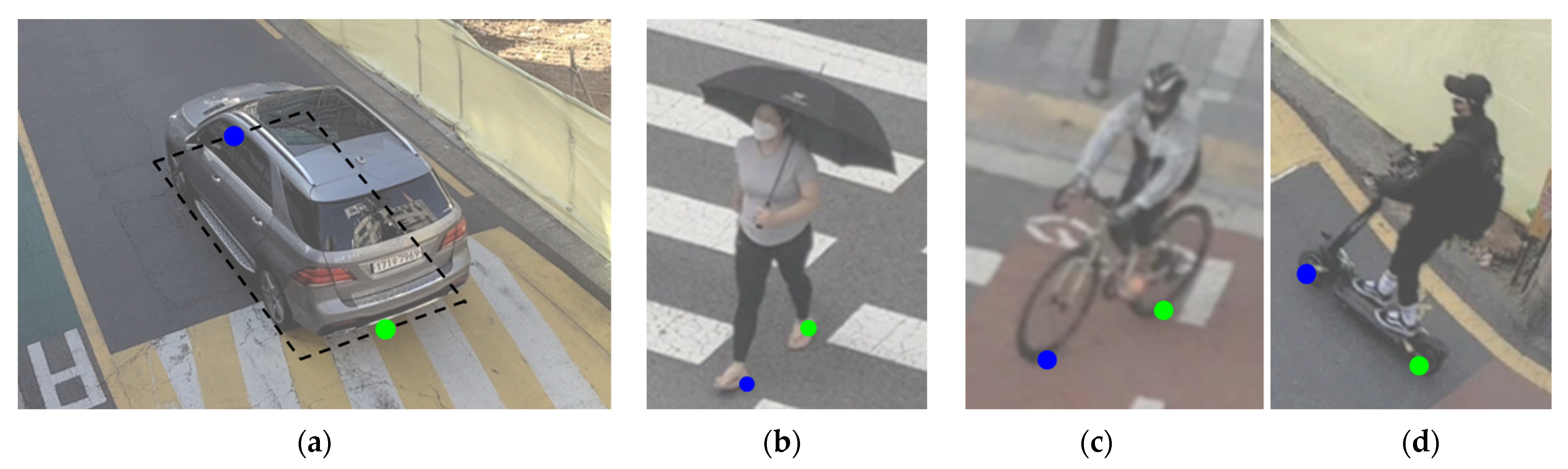
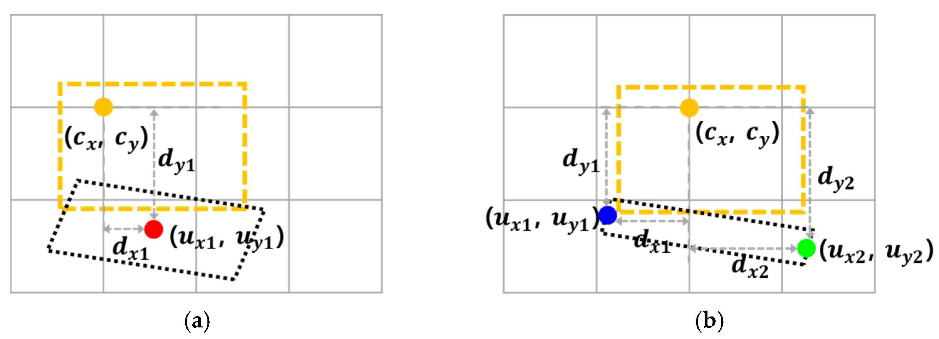
3.1. Definition of the One-Point

The one-point is the imaged location of a road user’s bottom face center in world coordinates. Figure 3 shows how the one-point is defined for each road user type. The black dotted quadrilateral and red circle in each figure are the images of the road user’s bottom face and its center in world coordinates, respectively. In the case of the car, its bottom face is defined as a rectangle formed by its outer boundary (as shown in Figure 3a). In the case of the pedestrian, their foot (particularly the heel) is regarded as the ground contact point. Although two feet cannot be guaranteed to meet the ground simultaneously depending on the walking phase, foot height over the ground surface is not so high that its effect is considered neglectable. As the bottom face of a walking pedestrian is narrow in the width direction, its bottom face can be approximated by a line connecting two feet (as shown in Figure 3b). In the case of the bicycle and e-scooter, its bottom face can be represented by a line connecting two wheel-ground contact points (as shown in Figure 3c) since its two wheels meet the ground. The one-point detector is implemented by the method described in Section 3.3, and its output is one coordinate.

3.2. Definition of the Two-Point

The two-points are the imaged locations of the front and rear center of a road user’s bottom face in world coordinates. Taking into account the characteristics of the road users, they are introduced to provide information about the road users’ location, size, and direction at minimal cost. The middle point of the two points could provide an accurate position like the one-point method. As the two points show the front and rear center of a road user’s bottom face, the line connecting the two points could provide information about the size and direction of the road user. Figure 4 shows how two-points are defined for each of the four road user types. In each figure, blue and green circles indicate the front and rear of the two-points, respectively. In the case of the car, the front and rear centers of the car’s bottom face are used as the two points (as shown in Figure 4a). In the case of the pedestrian, their foot (particularly the heel) is regarded as the ground contact point. As in the one-point definition, the effect of foot height over the ground surface is considered neglectable. Therefore, two feet are used as the two points (as shown in Figure 4b). For cyclists and e-scooter riders, two wheel-ground contact points are used as the two points (as shown in Figure 4c). The two-point detector is implemented using the method described in Section 3.3, and its output is two coordinates.

3.3. Implementation Details

This paper implements the proposed one-point and two-point detectors and compares their performances. Both detectors are implemented by adding extra heads to YOLOv7 [47].

3.3.1. Detector Implementation with YOLOv7

YOLOv7 is one of the various variants of YOLO and has shown fast detection speed and excellent performance in object detection in different application fields. For this reason, this paper uses YOLOv7 to implement the one-point and the two-point detectors. The structure of the two detectors is shown in Figure 5. The overall network structure is similar to that of YOLOv7: it consists of a backbone, neck, and heads. The backbone of the network is Efficient Layer Aggregation Network (ELAN) [48] modules trained on the COCO dataset [49]. The neck of the network is a combination of Feature Pyramid Network (FPN) [40] and Path Aggregation Network (PANet) [50] with ELAN and Cross Stage Partial Network (CSPNet) [51] modules. Specifically, it consists of Spatial Pyramid Pooling with Cross Stage Partial Network (SPPCSPC) [47], Convolution with Batch Normalization and SiLU (CBS), upsampling, concatenation, ELAN, Max Pooling (MP), and Re-parameterization Convolution (RepConv) modules.

The head consists of the original head of YOLOv7 (denoted by Y_x) and the extra heads added in this paper (denoted by Ŷ_x,k). As in the original YOLOv7, three heads are used for three different scales: small, medium, and large. The subscript X of Y_x and Ŷ_x,k represents the scale and will be one of S, M, and L, respectively. Y_x (depicted by green blocks in Figure 5) plays the same role as in the original YOLOv7 and contains the location, size, confidence score, and class of the bounding box. Heads added to provide additional information (i.e., one point or two points) are not used universally for all classes (which are road user types in our application) but are added for each class. In other words, extra heads for four road user types are allocated separately, and which heads will be used is determined by the class of Y_x or the ground truth. The extra heads selected by the class will be used for the inference and training, and the other extra heads will be ignored. The extra heads are denoted by Ŷ_x,k, and the subscript k represents the class: C (Car), P (pedestrian), B (cyclist), or E (e-scooter rider). They are depicted by red, yellow, blue, and sky-blue blocks in Figure 5. This allows for the use of different weights for each class during training. Finally, the only difference between the one-point and two-point detectors is the output size of the extra heads: the one-point detector outputs one coordinate, and the two-point detector outputs two coordinates.

3.3.2. Output Format of the One-Point and Two-Point Detectors

The one-point detector outputs one coordinate, and the two-point detector outputs two coordinates and their order. The points’ order is represented by a binary class since the two coordinates represent the front and rear in order or the reverse order. The order is encoded by applying the sigmoid function to one assigned output of the extra heads.

These coordinates output of both detectors use the same encoding scheme. The target location (${\mathit{u}}_{\mathit{x}}$, ${\mathit{u}}_{\mathit{y}}$) is expressed as the sum of its reference point and the offset from the reference point. In this paper, the reference point (c_x, c_y) is defined as the upper left corner of the grid cell responsible for the interesting object. Which grid cell is responsible for a certain object is determined by the feature map decoding method of YOLOv7. The offset (d_x, d_y) is obtained based on the method for calculating the center of the bounding box in YOLOv7 as

$${\mathit{u}}_{\mathit{x}\mathit{i}}={\mathit{c}}_{\mathit{x}}+{\mathit{d}}_{\mathit{x}\mathit{i}}, {\mathit{u}}_{\mathit{y}\mathit{i}}={\mathit{c}}_{\mathit{y}}+{\mathit{d}}_{\mathit{y}\mathit{i}}, i=1, 2, \mathrm{where} {\mathit{d}}_{\mathit{x}\mathit{i}} = 2 {\mathit{v}}_{\mathit{x}} -0.5, {\mathit{d}}_{\mathit{y}\mathit{i}} = 2 {\mathit{v}}_{\mathit{y}} -0.5$$

(1)

where the subscript i denotes the point index: in the case of the one-point detector, i = 1, and in the case of the two-point detector, i = 1 or 2. v_x and v_y are the output of the extra heads.

Figure 6 shows how this encoding scheme can be used for the one-point and two-point detectors, respectively. The yellow dotted rectangle and yellow dot depict the anchor box and the reference point, respectively. In Figure 6a, the black-dotted quadrilateral and red dot depict the object’s bottom face and its center, respectively. It shows how the offset is defined for the center. Similarly, in Figure 6b, the black dotted quadrilateral and two dots (blue dot and green dot) depict the object’s bottom face and its two points, respectively. It shows how two offsets are defined for the two points.

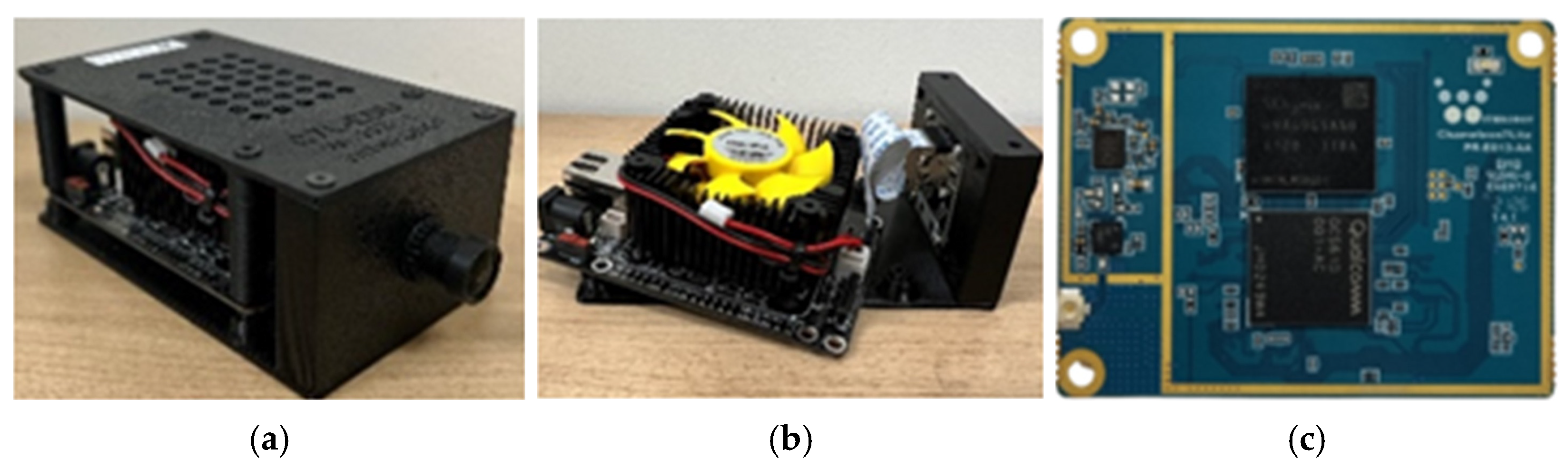
3.4. Network Simplification and Embedding

Network simplification is necessary to apply the proposed method to real-time embedded systems. Simplification methods include the light-weight model method [52], which reduces the size by changing the model structure, and the model compression method [53], which removes unnecessary parameters. While the light-weight model method involves the inconvenience of redesigning the model structure, the model compression method is easy to apply because it uses the structure of the existing model. This paper uses network pruning, the most widely used model compression method [54]. It removes connections or weights with low importance from the model to reduce the number of parameters and computation amounts. While it includes pruning by channel, layer, and weight, this paper uses pruning by channel.

Pruning by channel is performed using the Torch-Pruning library [55]. Torch-Pruning is a network pruning library designed for light-weight deep learning models based on PyTorch v3.9. This is a DepGraph-based method [56] that automatically performs complex graph restructuring and parameter rearrangement during model pruning. Additionally, it provides various evaluation methods for importance, such as magnitude, L1/L2 norm, and random. Among them, this paper uses channel pruning based on random importance. It generates random numbers from a uniform distribution between zero and one and assigns these random values as the importance of each channel of the convolution filters. Channels with low importance are sequentially removed, and fine-tuning is performed to compensate for the performance degradation caused by pruning, resulting in a simplified model.

This paper embeds the simplified model into an AI camera (incorporating Qualcomm QCS610 SoC) to confirm that it operates on the edge device in real time. The system is measured to consume only 3.6 W (=300 mA × 12 V) while operating the road user detector, which can satisfy the harsh power consumption requirement of traffic monitoring equipment. Figure 7 shows an AI camera incorporating an embedded board with QCS610 SoC, which includes a Kyro 460 CPU, Adreno 612 GPU, and Hexagon 685 DSP. The software is developed using Qualcomm’s Snapdragon Neural Processing Engine (SNPE), a software framework designed to run deep neural networks. The embedding process [57] is as follows. First, the simplified model is converted to a Deep Learning Container (DLC) file format. In the meantime, parameter quantization is required to convert to a DLC file. This is because DSP supports only 8-bit integer operation while DLC files store model parameters in floating point format. In this paper, for the parameter quantization, the Post Training Quantization (PTQ) provided by SNPE is applied. Finally, onboard inference is performed by importing the quantized DLC file into the embedded board.

4. Experimental Results

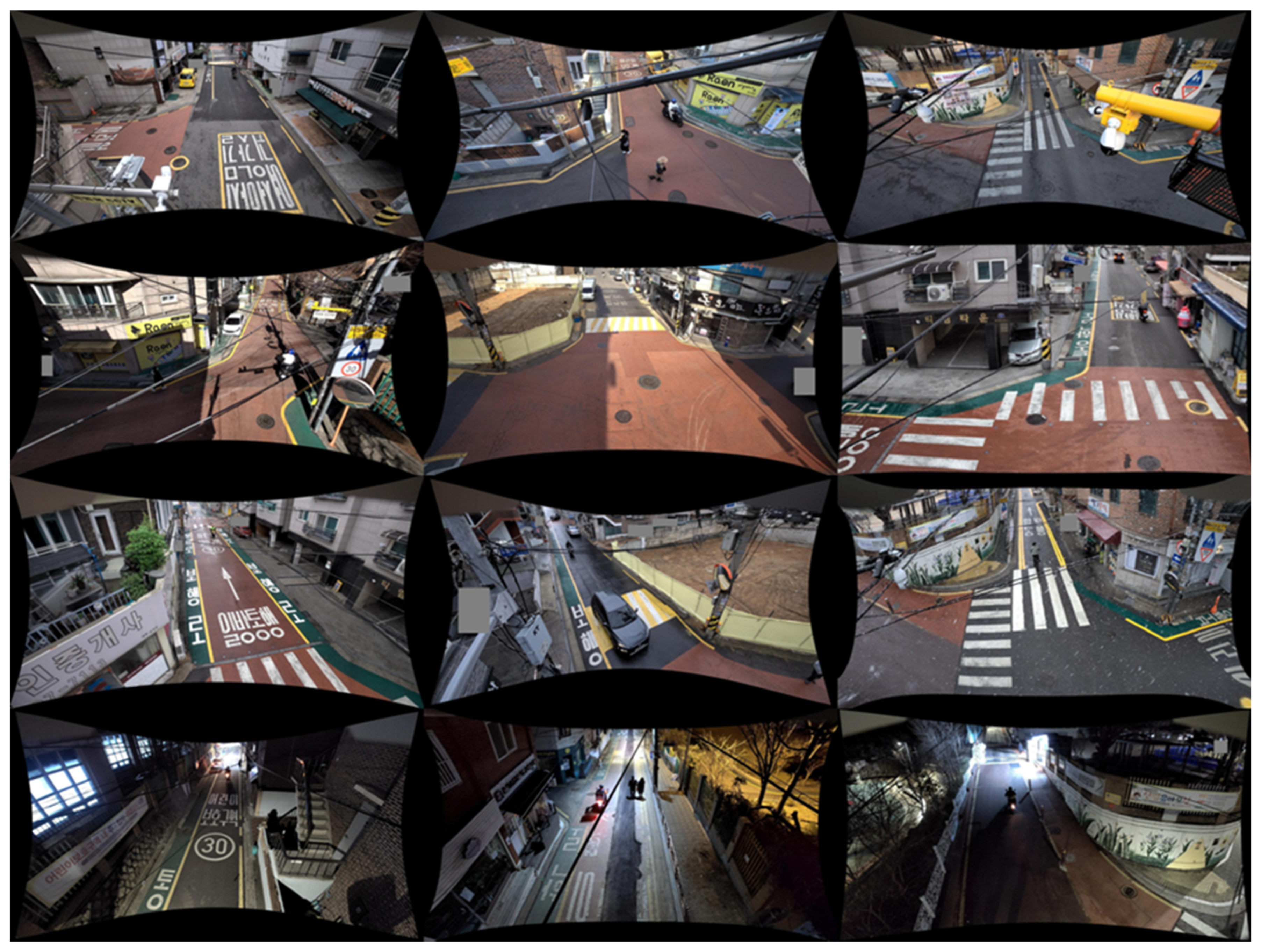
4.1. Experimental Setup

The dataset used for the experiment consists of customized data acquired by authors and data selected from the public dataset. The customized data were captured by surveillance cameras at 16 different locations, where the postures of the cameras relative to the ground surface varied. They were taken from December 2020 to April 2023 to reflect various seasonal and lighting conditions. In addition, images were used after removing fisheye lens distortion using the method in [58]. Figure 8 shows example images of the customized data. As shown in the figure, the dataset includes road users in various directions. Since the customized data includes insufficient e-scooter rider samples, the data selected from AIHUB [59] has been used to supplement it. The images in this data were captured by surveillance cameras at two different locations. Figure 9 shows example images of the data from AIHUB. As shown in the figure, all other road users except e-scooter riders were masked with gray-filled bounding boxes. The dataset was divided into training and test sets, which included 11,434 and 2017 images, respectively.

Table 1. Number of images in the datasets.

	Training	Test
Customized	9752	1724
AIHUB	1682	293
Total	11434	2017

shows the number of images in the dataset. The training and test sets include 31,003 and 5370 objects, respectively.

Table 2. Statistics of four road user types in the dataset.

	Car	Pedestrian	Cyclist	e-Scooter	Total
Training	9073	9734	8869	3327	31,003
Test	1665	1617	1555	533	5370

shows detailed statistics of four road user types in the dataset.

In the case of the car, to obtain the ground truth of bottom face centers and user-specific two locations, this paper utilized a geometric relation between the camera and the ground surface as well as the car size. The geometric relation was calibrated based on [60,61], which use parallel lines on images. Knowing the geometric relation between the camera and the ground surface, a 3D bounding box with a specific size can be projected onto the 2D image. Starting from the initial 3D bounding box (as inferred from the car type), its position, direction, and size are finely adjusted to make it more suitable for human viewing. Once the 3D bounding box is fixed, the center point of the car or the front and rear bottom centers of the car can be easily calculated based on the 3D bounding box.

Training settings are as follows: SGD optimizer, epoch = 400, and batch size = 18. Both training and evaluation were performed using Pytorch and NVIDIA GeForce RTX 3090. Non-English words in this figure do not relate to the proposed method. Thus, they do not need any explanation.

4.2. Evaluation and Analysis

The position error of the proposed methods is evaluated using mean position error (mPE). The mPE is defined as

$$\mathrm{m}\mathrm{P}\mathrm{E}={\displaystyle \frac{1}{N}}\sum _{i=1}^N\sqrt{{\left({\displaystyle \frac{x_i-{\widehat{x}}_i}{W_i}}\right)}^2+{\left({\displaystyle \frac{y_i-{\widehat{y}}_i}{H_i}}\right)}^2}$$

(2)

where $N$ represents the total number of road users while $(x_i,y_i)$ and $({\widehat{x}}_i,{\widehat{y}}_i)$ refer to the ground truth point and the estimation result, respectively. (W_i, H_i) indicates the size of the road user’s bounding box. Consequently, the mPE can be thought of as the position error when the bounding box size is $1\times 1$ or the position error ratio with respect to the size of the bounding box.

Table 3. Performance comparison of the existing and proposed methods. The mPE of the two-point detectors was calculated using the center of the two points.

Class	Existing Method		One-Point Detector		Two-Point Detector
	AP	mPE	AP	mPE	AP	mPE
Car	99.32%	0.3609	99.29%	0.0654	99.21%	0.0710
Pedestrian	83.81%	0.1750	82.92%	0.1153	82.29%	0.1201
Cyclist	99.38%	0.2045	98.90%	0.0682	98.67%	0.0741
E-scooter	97.66%	0.1742	98.25%	0.0948	95.99%	0.1011
Average	95.04% (mAP)	0.2452	94.84% (mAP)	0.0821	94.04% (mAP)	0.0875

shows the Average Precision (AP) and mPE of the existing and proposed methods. The existing method determines the road user’s location as the bottom center of the bounding box. The proposed method utilizes the detection results of the one-point and two-point detectors. To ensure an equivalent comparison with the one-point detector, we calculated mPE using the center of the two points detected by the two-point detector. As demonstrated in Table 3, both the one-point detector (mPE = 0.0821) and the two-point detector (mPE = 0.0875) outperformed the existing method (mPE = 0.2452) in terms of the position error, showing similar detection performances. The mPE of the one-point detector is reduced by 66.5% compared to the mPE of the existing method. The one-point and two-point detectors show similar mAP and mPE. For both detectors, cars and cyclists exhibit relatively lower mPE for both detectors than pedestrians and e-scooters. Even if the positioning accuracies of the two detectors are similar, the two-point detector can provide information about the size and direction of the road user. This additional information can be helpful in tracking because detected road users in consecutive frames can be associated using not only their locations but also their sizes and directions.

Figure 10 shows the detection results of the one-point detector. Cars, pedestrians, cyclists, and e-scooter riders are depicted by bounding boxes in blue, green, yellow, and magenta, respectively. The ground truth is displayed in gray. A filled circle represents the detected one-point. This figure demonstrates that the one-point detector successfully detects the position of road users in different locations, times, and weather conditions, as well as in various moving directions. Figure 11 shows the detection results of the two-point detector. Bounding boxes are depicted in the same color as Figure 10. Unlike the one-point detector, the two-point detector provides the positions of the two points and their order. To distinguish the order of the two points, the front and rear points are represented by empty and filled circles, respectively. The detection results in this figure show that the two-point detector also successfully finds the positions of the target objects in various situations.

When calculating the mPE for the two-point detector, the order of the two points can be imposed or ignored. When the order is used, mPE is denoted by mPE_Ordered and calculated by considering the order prediction result. In the case where the order is not used, mPE is denoted by mPE_Orderless and calculated by finding adjacent pairs. It is important to note that mPE_Orderless differs from mPE as two points are used individually instead of using their mean location. The mPE_Ordered is the average of the front and rear mPE. The front mPE is calculated using the point labeled as front in the ground truth and the point predicted as front by the two-point detector, and the rear mPE is calculated using the point labeled as rear in the ground truth and the point predicted as rear. The mPE_Ordered is calculated as

$${mPE}_{Ordered}={\displaystyle \frac{1}{N}}\sum _{i=1}^N{\displaystyle \frac{1}{2}}\left\{\sqrt{{\left({\displaystyle \frac{x_{i,f}-{\widehat{x}}_{i,f}}{W_i}}\right)}^2+{\left({\displaystyle \frac{y_{i,f}-{\widehat{y}}_{i,f}}{H_i}}\right)}^2}+\sqrt{{\left({\displaystyle \frac{x_{i,r}-{\widehat{x}}_{i,r}}{W_i}}\right)}^2+{\left({\displaystyle \frac{y_{i,r}-{\widehat{y}}_{i,r}}{H_i}}\right)}^2}\right\}$$

(3)

where $N$ is the total number of road users. $(x_{i,f},y_{i,f})$ and $({\widehat{x}}_{i,f},{\widehat{y}}_{i,f})$ refer to the ground truth and the detected front point, respectively. $(x_{i,r},y_{i,r})$ and $({\widehat{x}}_{i,r},{\widehat{y}}_{i,r})$ refer to the ground truth and the detected rear point, respectively.

The mPE_Orderless is calculated by matching each predicted point to the nearby ground truth instead of using the predicted order and calculated as

$${mPE}_{Orderless}={\displaystyle \frac{1}{N}}\sum _{i=1}^N{\displaystyle \frac{1}{2}}\left\{\sqrt{{\left({\displaystyle \frac{x_{i,f}-{\widehat{x}}_{i,o_1}}{W_i}}\right)}^2+{\left({\displaystyle \frac{y_{i,f}-{\widehat{y}}_{i,o_1}}{H_i}}\right)}^2}+\sqrt{{\left({\displaystyle \frac{x_{i,r}-{\widehat{x}}_{i,o_2}}{W_i}}\right)}^2+{\left({\displaystyle \frac{y_{i,r}-{\widehat{y}}_{i,o_2}}{H_i}}\right)}^2}\right\}$$

(4)

where $N$ is the total number of road users. $(x_{i,f},y_{i,f})$ and $(x_{i,r},y_{i,r})$ represent the ground truth front and rear points, respectively. $({\widehat{x}}_{i,o_1},{\widehat{y}}_{i,o_1})$ and $({\widehat{x}}_{i,o_2},{\widehat{y}}_{i,o_2})$ represent the output points matched based on the distance from the ground truth.

Table 4. mPE_Ordered and mPE_Orderless of the two-point detector.

Class	Two-Point Detector’s Results
	mPEOrdered	mPEOrderless
Car	0.1061	0.0993
Pedestrian	0.1760	0.1452
Cyclist	0.1119	0.1023
E-scooter	0.1405	0.1224
Average	0.1291	0.1142

shows mPE_Ordered and mPE_Orderless of the two-point detector. It can be seen that mPE_Ordered is larger than mPE_Orderless. This is because cases where the order is predicted in reverse, such as Figure 12, can occur. The empty and filled circles in Figure 12 represent the front and rear points, respectively. As the order prediction failed, it is evident that the mPE_Ordered has a large value because the predicted and ground truth results in the opposite direction.

Contrarily, the order information of the two points can be used to estimate the moving direction of the road user. Figure 13 shows moving directions estimated using the two-point order for a car, cyclist, and e-scooter rider. Blue, yellow, and magenta arrows indicate the estimated moving directions for the car, cyclist, and e-scooter rider, respectively, while red arrows indicate the actual moving directions. It can be noticed that the actual and estimated directions are similar. However, direction estimation using the two-point method is limited for pedestrians. Figure 14 shows moving directions estimated by the two-point order for pedestrians. Green and red arrows indicate the estimated and actual moving directions, respectively. In the pedestrian poses shown in Figure 14a, the green and red arrows point in the same direction, but they are not in the pedestrian poses shown in Figure 14b.

Figure 15 shows three primary reasons for the failure of the proposed method. Gray and color boxes indicate ground truth and detection results, respectively. In this figure, (a), (b), and (c) indicate failure cases caused by occlusion, low-resolution, and background with similar color, respectively. These three situations mostly degraded the detection performance of small-sized road users such as pedestrians. Furthermore, the proposed method has been applied to images captured in daytime, nighttime, and rainy situations. However, it was found that these situations do not noticeably degrade its performance compared to occlusion, low-resolution, and background.

4.3. Network Simplification and Embedding

Channel pruning was performed using the Random Importance method. The one-point and two-point detectors were pruned with different target speed-ups, which refers to the speed ratio of the simplified and baseline models. This paper increased the target speed-up value up to four because the two detectors showed real-time operability with 10 FPS on QCS610 SoC at this speed-up value. After pruning, the two detectors were fine-tuned with 400 epochs.

Table 5. Simplification and embedding results of the one-point detector on the QCS610 SoC.

Target Speed-Up	mAP (%)	mPE	FPS	Model Size (MB)	GFLOPs
1 (baseline)	94.70	0.1147	4.85	71.44	98.23
2	94.21	0.1138	7.03	35.28	48.63
3	92.64	0.1086	7.86	23.64	32.05
4	91.51	0.1211	10.61	17.65	23.71

presents the results of running the one-point detector using QCS610 SoC after applying network simplification and embedding. This table demonstrates the changes in mAP, position error, parameter size, FLOPs, and model size as the target speed-up varies. The target speed-up one represents the model with no pruning. As shown in Table 5, the target speed-up four results in a decrease of 3.19 in mAP, an increase of 0.0064 in mPE, and an increase of 5.76 in FPS compared to the baseline model. Moreover, the model size and GFLOPs decrease as the target speed-up increases, indicating the potential for significant computational savings.

Table 6. Simplification and embedding results of the two-point detector on the QCS610 SoC.

Target Speed-Up	mAP (%)	mPE	mPEOrdered	mPEOrderless	FPS	Model Size (MB)	GFLOPs
1 (baseline)	93.46	0.1058	0.1541	0.1399	4.90	71.60	98.49
2	91.91	0.1076	0.1567	0.1417	6.62	35.04	48.59
3	91.28	0.1042	0.1496	0.1385	8.44	24.21	32.66
4	89.30	0.1060	0.1553	0.1404	10.17	18.63	24.39

presents the results of running the two-point detector using QCS610 SoC after applying network simplification and embedding. As with the one-point detector, mAP decreases by up to 4.16 while mPE, mPE_Ordered, and mPE_Orderless maintain similar levels as the target speed-up increases. At the target speed-up of 4, FPS increases by up to 5.27, and the model size and GLOPs decrease by up to 52.97 and 74.10, respectively.

For pedestrians, the positioning error of the two-point detector is higher than that of the other road users. It is mainly because the dynamic nature of their movement makes it challenging to detect two points consistently. Thus, in the case of pedestrians, the one-point detector is advantageous over the two-point detector if it is not necessary to estimate the moving direction for the following reasons: One is that the accuracy of predicting the order of two points is relatively low, which may limit the practical effectiveness of the two-point detector. The other is that mAP of the two-point detector degrades more severely when the target speed-up increases compared to the one-point detector as shown in Table 5 and Table 6.

Table 7. Class-wise detection results of the one-point detector on QCS610 SoC.

Target Speed-Up	One-Point Detector’s Results
	Car AP (%)	Pedestrian AP (%)	Cyclist AP (%)	E-Scooter AP (%)	mAP (%)
1 (baseline)	99.10%	83.10%	99.00%	97.60%	94.70%
2	99.20%	81.40%	98.50%	97.80%	94.20%
3	99.10%	77.90%	98.70%	94.90%	92.60%
4	98.60%	73.60%	98.10%	95.70%	91.50%

and

Table 8. Class-wise detection results of the two-point detector on QCS610 SoC.

Target Speed-Up	Two-Point Detector’s Results
	Car AP (%)	Pedestrian AP (%)	Cyclist AP (%)	E-Scooter AP (%)	mAP (%)
1 (baseline)	99.00%	81.80%	98.60%	93.46%	93.50%
2	98.80%	76.60%	98.20%	94.10%	91.91%
3	98.50%	74.40%	97.90%	94.30%	91.28%
4	97.80%	69.60%	97.00%	92.70%	89.30%

show the class-wise detection performances used to compute the mAPs in Table 5 and Table 6, respectively. In Table 7 and Table 8, it can be observed that the pedestrian detection performance decreases the most as the target speed-up increases. This is mainly because pedestrians are relatively small in images and their appearance changes significantly depending on posture. However, as shown in Table 5 and Table 6, the mPE maintains similar values as the target speed-up increases. It is important to note that since the mPE is calculated only for the correctly detected objects, the performance degradation due to the target speed-up may not be fully reflected.

5. Conclusions

This paper proposes a method for enhancing the positioning accuracy of various road users by minimally modifying a conventional object detector to extract one or two object-specific key points. The proposed method has the following advantages from the practicality viewpoint: (1) It improves the positioning accuracy of four types of road users by detecting the bottom face centers and user-specific two points via adding only extra heads to a conventional object detector. (2) It can operate on the edge device in real time because it negligibly increases the computational cost of the conventional object detector. The experimental results showed that the proposed method could improve the positioning accuracy of four types of road users and be embedded on the edge camera with a Qualcomm QCS 610 SoC. In the future, we plan to apply the proposed method to real-world ITS applications and investigate the effect of the positioning accuracy improvement on the performance of the final application. Furthermore, we plan to reimplement the proposed method based on a higher version detector, such as YOLOv10 or YOLOv11, and embed them on edge devices to check their real-time operability. We also consider applying YOLO-Pose to enhance the accuracy of the two key points of pedestrians. In addition, we plan to combine the proposed method with post-processing techniques such as the Kalman filter or recurrent neural network (RNN) and explore an approach of treating e-scooters and the other two-wheelers as separate classes by reflecting their structural characteristics.

References

1. Yu, H.; Luo, Y.; Shu, M.; Huo, Y.; Yang, Z.; Shi, Y.; Guo, Z.; Li, H.; Hu, X.; Yuan, J. Dair-v2x: A large-scale dataset for vehicle-infrastructure cooperative 3D object detection. In Proceedings of the IEEE/CVF Conference on Computer Vision and Pattern Recognition, New Orleans, LA, USA, 18–24 June 2022; pp. 21361–21370. [Google Scholar]
2. Cong, Z.; Li, K.; Zhang, R.; Peng, T.; Zong, C. Phase diagram in multi-phase heterogeneous traffic flow model integrating the perceptual range difference under human-driven and connected vehicles environment. Chaos Solitons Fractals 2024, 182, 114791. [Google Scholar]
3. Ku, J.; Mozifian, M.; Lee, J.; Harakeh, A.; Waslander, S.L. Joint 3d proposal generation and object detection from view aggregation. In Proceedings of the 2018 IEEE/RSJ International Conference on Intelligent Robots and Systems (IROS), Madrid, Spain, 1–5 October 2018; pp. 1–8. [Google Scholar]
4. Chen, X.; Ma, H.; Wan, J.; Li, B.; Xia, T. Multi-view 3d object detection network for autonomous driving. In Proceedings of the IEEE Conference on Computer Vision and Pattern Recognition, Honolulu, HI, USA, 21–26 July 2017; pp. 1907–1915. [Google Scholar]
5. Zhang, Y.; Lu, J.; Zhou, J. Objects are different: Flexible monocular 3d object detection. In Proceedings of the IEEE/CVF Conference on Computer Vision and Pattern Recognition, Nashville, TN, USA, 20–25 June 2021; pp. 3289–3298. [Google Scholar]
6. Brazil, G.; Liu, X. M3d-rpn: Monocular 3d region proposal network for object detection. In Proceedings of the IEEE/CVF International Conference on Computer Vision, Seoul, Republic of Korea, 27 October–2 November 2019; pp. 9287–9296. [Google Scholar]
7. Liu, C.; Huynh, D.Q.; Sun, Y.; Reynolds, M.; Atkinson, S. A vision-based pipeline for vehicle counting, speed estimation, and classification. IEEE Trans. Intell. Transp. Syst. 2020, 22, 7547–7560. [Google Scholar]
8. Wang, C.; Musaev, A. Preliminary research on vehicle speed detection using traffic cameras. In Proceedings of the IEEE International Conference on Big Data (Big Data), Los Angeles, CA, USA, 9–12 December 2019; pp. 3820–3823. [Google Scholar]
9. Giannakeris, P.; Kaltsa, V.; Avgerinakis, K.; Briassouli, A.; Vrochidis, S.; Kompatsiaris, I. Speed estimation and abnormality detection from surveillance cameras. In Proceedings of the IEEE Conference on Computer Vision and Pattern Recognition Workshops, Salt Lake City, UT, USA, 18–23 June 2018; pp. 93–99. [Google Scholar]
10. Gupta, I.; Rangesh, A.; Trivedi, M. 3D Bounding Boxes for Road Vehicles: A One-Stage, Localization Prioritized Approach using Single Monocular Images. In Proceedings of the European Conference on Computer Vision (ECCV) Workshops, Munich, Germany, 8–14 September 2018. [Google Scholar]
11. Zhang, B.; Zhang, J. A traffic surveillance system for obtaining comprehensive information of the passing vehicles based on instance segmentation. IEEE Trans. Intell. Transp. Syst. 2020, 22, 7040–7055. [Google Scholar]
12. Li, B.; Ouyang, W.; Sheng, L.; Zeng, X.; Wang, X. Gs3d: An efficient 3d object detection framework for autonomous driving. In Proceedings of the IEEE/CVF Conference on Computer Vision and Pattern Recognition, Long Beach, CA, USA, 15–20 June 2019; pp. 1019–1028. [Google Scholar]
13. Fang, J.; Zhou, L.; Liu, G. 3d bounding box estimation for autonomous vehicles by cascaded geometric constraints and depurated 2d detections using 3d results. arXiv 2019, arXiv:1909.01867. [Google Scholar]
14. Zhu, M.; Zhang, S.; Zhong, Y.; Lu, P.; Peng, H.; Lenneman, J. Monocular 3d vehicle detection using uncalibrated traffic cameras through homography. In Proceedings of the 2021 IEEE/RSJ International Conference on Intelligent Robots and Systems (IROS), Prague, Czech Republic, 27 September 2021; pp. 3814–3821. [Google Scholar]
15. Kim, G.; Jung, H.G.; Suhr, J.K. CNN-Based Vehicle Bottom Face Quadrilateral Detection Using Surveillance Cameras for Intelligent Transportation Systems. Sensors 2023, 23, 6688. [Google Scholar] [CrossRef]
16. Gählert, N.; Wan, J.J.; Weber, M.; Zöllner, J.M.; Franke, U.; Denzler, J. Beyond bounding boxes: Using bounding shapes for real-time 3d vehicle detection from monocular rgb images. In Proceedings of the 2019 IEEE Intelligent Vehicles Symposium (IV), Paris, France, 9–12 June 2019; pp. 675–682. [Google Scholar]
17. Qin, Z.; Wang, J.; Lu, Y. Monogrnet: A geometric reasoning network for monocular 3d object localization. Proc. AAAI Conf. Artif. Intell. 2019, 33, 8851–8858. [Google Scholar]
18. Carrillo, J.; Waslander, S. Urbannet: Leveraging urban maps for long range 3d object detection. In Proceedings of the 2021 IEEE International Intelligent Transportation Systems Conference (ITSC), Indianapolis, IN, USA, 19–22 September 2021; pp. 3799–3806. [Google Scholar]
19. Li, P.; Zhao, H.; Liu, P.; Cao, F. Rtm3d: Real-time monocular 3d detection from object keypoints for autonomous driving. In Proceedings of the European Conference on Computer Vision, Glasgow, UK, 23–28 August 2020; pp. 644–660. [Google Scholar]
20. Tang, X.; Wang, W.; Song, H.; Zhao, C. CenterLoc3D: Monocular 3D vehicle localization network for roadside surveillance cameras. Complex Intell. Syst. 2023, 9, 4349–4368. [Google Scholar]
21. Weber, M.; Fürst, M.; Zöllner, J.M. Direct 3d detection of vehicles in monocular images with a cnn based 3d decoder. In Proceedings of the 2019 IEEE Intelligent Vehicles Symposium (IV), Paris, France, 9–12 June 2019; pp. 417–423. [Google Scholar]
22. Liu, Z.; Wu, Z.; Tóth, R. Smoke: Single-stage monocular 3d object detection via keypoint estimation. In Proceedings of the IEEE/CVF Conference on Computer Vision and Pattern Recognition Workshops, Seattle, WA, USA, 14–19 June 2020; pp. 996–997. [Google Scholar]
23. Jiaojiao, F.; Linglao, Z.; Guizhong, L. Monocular 3D Detection for Autonomous Vehicles by Cascaded Geometric Constraints and Depurated Using 3D Results. In Proceedings of the 2020 3rd International Conference on Unmanned Systems (ICUS), Harbin, China, 27–28 November 2020; pp. 954–959. [Google Scholar]
24. Mauri, A.; Khemmar, R.; Decoux, B.; Haddad, M.; Boutteau, R. Lightweight convolutional neural network for real-time 3D object detection in road and railway environments. J. Real-Time Image Process. 2022, 19, 499–516. [Google Scholar]
25. Liu, W.; Anguelov, D.; Erhan, D.; Szegedy, C.; Reed, S.; Fu, C.Y.; Berg, A.C. Ssd: Single shot multibox detector. In Proceedings of the Computer Vision–ECCV 2016: 14th European Conference, Amsterdam, The Netherlands, 11–14 October 2016; pp. 21–37. [Google Scholar]
26. Duan, K.; Bai, S.; Xie, L.; Qi, H.; Huang, Q.; Tian, Q. Centernet: Keypoint triplets for object detection. In Proceedings of the IEEE/CVF International Conference on Computer Vision, Seoul, Republic of Korea, 27 October–2 November 2019; pp. 6569–6578. [Google Scholar]
27. Mousavian, A.; Anguelov, D.; Flynn, J.; Kosecka, J. 3d bounding box estimation using deep learning and geometry. In Proceedings of the IEEE Conference on Computer Vision and Pattern Recognition, Honolulu, HI, USA, 21–26 July 2017; pp. 7074–7082. [Google Scholar]
28. Ahmed, S.; Huda, M.N.; Rajbhandari, S.; Saha, C.; Elshaw, M.; Kanarachos, S. Pedestrian and cyclist detection and intent estimation for autonomous vehicles: A survey. Appl. Sci. 2019, 9, 2335. [Google Scholar] [CrossRef]
29. Li, X.; Li, L.; Flohr, F.; Wang, J.; Xiong, H.; Bernhard, M.; Pan, S.; Gavrila, D.M.; Li, K. A unified framework for concurrent pedestrian and cyclist detection. IEEE Trans. Intell. Transp. Syst. 2016, 18, 269–281. [Google Scholar]
30. Zhou, C.; Yuan, J. Bi-box regression for pedestrian detection and occlusion estimation. In Proceedings of the European Conference on Computer Vision (ECCV), Munich, Germany, 8–14 September 2018; pp. 135–151. [Google Scholar]
31. Cai, J.; Lee, F.; Yang, S.; Lin, C.; Chen, H.; Kotani, K.; Chen, Q. Pedestrian as points: An improved anchor-free method for center-based pedestrian detection. IEEE Access 2020, 8, 179666–179677. [Google Scholar] [CrossRef]
32. Fang, H.S.; Xie, S.; Tai, Y.W.; Lu, C. Rmpe: Regional multi-person pose estimation. In Proceedings of the IEEE International Conference on Computer Vision, Venice, Italy, 22–29 October 2017; pp. 2334–2343. [Google Scholar]
33. He, K.; Gkioxari, G.; Dollár, P.; Girshick, R. Mask r-cnn. In Proceedings of the IEEE International Conference on Computer Vision, Venice, Italy, 22–29 October 2017; pp. 2961–2969. [Google Scholar]
34. Chen, Y.; Wang, Z.; Peng, Y.; Zhang, Z.; Yu, G.; Sun, J. Cascaded pyramid network for multi-person pose estimation. In Proceedings of the IEEE Conference on Computer Vision and Pattern Recognition, Salt Lake City, UT, USA, 18–23 June 2018; pp. 7103–7112. [Google Scholar]
35. Rezaei, M.; Azarmi, M.; Mir, F.M.P. Traffic-Net: 3D traffic monitoring using a single camera. arXiv 2021, arXiv:2109.09165 2021. [Google Scholar] [CrossRef]
36. Liu, X.; Xue, N.; Wu, T. Learning auxiliary monocular contexts helps monocular 3d object detection. Proc. AAAI Conf. Artif. Intell. 2022, 36, 1810–1818. [Google Scholar]
37. Mauri, A.; Khemmar, R.; Decoux, B.; Haddad, M.; Boutteau, R. Real-time 3D multi-object detection and localization based on deep learning for road and railway smart mobility. J. Imaging 2021, 7, 145. [Google Scholar] [CrossRef] [PubMed]
38. Li, X.; Flohr, F.; Yang, Y.; Xiong, H.; Braun, M.; Pan, S.; Li, K.; Gavrila, D.M. A new benchmark for vision-based cyclist detection. In Proceedings of the 2016 IEEE Intelligent Vehicles Symposium (IV), Gothenburg, Sweden, 19–22 June 2016; pp. 1028–1033. [Google Scholar]
39. Boonsirisumpun, N.; Puarungroj, W.; Wairotchanaphuttha, P. Automatic detector for bikers with no helmet using deep learning. In Proceedings of the 2018 22nd International Computer Science and Engineering Conference (ICSEC), Chiang Mai, Thailand, 21–24 November 2018; pp. 1–4. [Google Scholar]
40. Dollár, P.; Appel, R.; Belongie, S.; Perona, P. Fast feature pyramids for object detection. IEEE Trans. Pattern Anal. Mach. Intell. 2014, 36, 1532–1545. [Google Scholar] [CrossRef] [PubMed]
41. Felzenszwalb, P.F.; Girshick, R.B.; McAllester, D.; Ramanan, D. Object detection with discriminatively trained part-based models. IEEE Trans. Pattern Anal. Mach. Intell. 2009, 32, 1627–1645. [Google Scholar] [CrossRef]
42. Girshick, R. Fast r-cnn. In Proceedings of the IEEE International Conference on Computer Vision, Santiago, Chile, 7–13 December 2015; pp. 1440–1448. [Google Scholar]
43. Chen, H.H.; Lin, C.C.; Wu, W.Y.; Chan, Y.M.; Fu, L.C.; Hsiao, P.Y. Integrating appearance and edge features for on-road bicycle and motorcycle detection in the nighttime. In Proceedings of the 17th International IEEE Conference on Intelligent Transportation Systems (ITSC), Qingdao, China, 8–11 October 2014; pp. 354–359. [Google Scholar]
44. Apurv, K.; Tian, R.; Sherony, R. Detection of e-scooter riders in naturalistic scenes. arXiv 2021, arXiv:2111.14060. [Google Scholar]
45. Gilroy, S.; Mullins, D.; Jones, E.; Parsi, A.; Glavin, M. E-scooter rider detection and classification in dense urban environments. Results Eng. 2022, 16, 100677. [Google Scholar] [CrossRef]
46. Ahmed, D.B.; Diaz, E.M. Survey of machine learning methods applied to urban mobility. IEEE Access 2022, 10, 30349–30366. [Google Scholar] [CrossRef]
47. Wang, C.Y.; Bochkovskiy, A.; Liao, H.Y.M. YOLOv7: Trainable bag-of-freebies sets new state-of-the-art for real-time object detectors. In Proceedings of the IEEE/CVF Conference on Computer Vision and Pattern Recognition, Vancouver, BC, Canada, 17–24 June 2023; pp. 7464–7475. [Google Scholar]
48. Wang, C.Y.; Liao, H.Y.M.; Yeh, I.H. Designing network design strategies through gradient path analysis. arXiv 2022, arXiv:2211.04800 2022. [Google Scholar]
49. Lin, T.Y.; Maire, M.; Belongie, S.; Hays, J.; Perona, P.; Ramanan, D.; Dollár, P.; Zitnick, C.L. Microsoft coco: Common objects in context. In Proceedings of the Computer Vision–ECCV 2014: 13th European Conference, Zurich, Switzerland, 6–12 September 2014; Part V, 13. pp. 740–755. [Google Scholar]
50. Liu, S.; Qi, L.; Qin, H.; Shi, J.; Jia, J. Path aggregation network for instance segmentation. In Proceedings of the IEEE Conference on Computer Vision and Pattern Recognition, Salt Lake City, UT, USA, 18–23 June 2018; pp. 8759–8768. [Google Scholar]
51. Wang, C.Y.; Liao, H.Y.M.; Wu, Y.H.; Chen, P.Y.; Hsieh, J.W.; Yeh, I.H. CSPNet: A new backbone that can enhance learning capability of CNN. In Proceedings of the IEEE/CVF Conference on Computer Vision and Pattern Recognition Workshops, Seattle, WA, USA, 14–19 June 2020; pp. 390–391. [Google Scholar]
52. Liu, Z.; Li, J.; Shen, Z.; Huang, G.; Yan, S.; Zhang, C. Learning efficient convolutional networks through network slimming. In Proceedings of the IEEE International Conference on Computer Vision, Venice, Italy, 22–29 October 2017; pp. 2736–2744. [Google Scholar]
53. Han, S.; Pool, J.; Tran, J.; Dally, W. Learning both weights and connections for efficient neural network. Adv. Neural Inf. Process. Syst. 2015, 28. [Google Scholar]
54. Lee, Y.; Moon, Y.H.; Park, J.Y.; Min, O.G. Recent R&D trends for lightweight deep learning. Electron. Telecommun. Trends 2019, 34, 40–50. [Google Scholar]
55. Torch-Pruning. Available online: https://github.com/VainF/Torch-Pruning (accessed on 8 May 2024).
56. Fang, G.; Ma, X.; Song, M.; Mi, M.B.; Wang, X. Depgraph: Towards any structural pruning. In Proceedings of the IEEE/CVF Conference on Computer Vision and Pattern Recognition, Vancouver, BC, Canada, 17–24 June 2023; pp. 16091–16101. [Google Scholar]
57. Lee, Y.J.; Jung, H.G.; Suhr, J.K. Semantic Segmentation Network Slimming and Edge Deployment for Real-Time Forest Fire or Flood Monitoring Systems Using Unmanned Aerial Vehicles. Electronics 2023, 12, 4795. [Google Scholar] [CrossRef]
58. Devernay, F.; Faugeras, O. Straight lines have to be straight. Mach. Vis. Appl. 2001, 13, 14–24. [Google Scholar]
59. AI Hub. Available online: https://www.aihub.or.kr/aihubdata/data/view.do?currMenu=&topMenu=&aihubDataSe=data&dataSetSn=169 (accessed on 21 March 2023).
60. Caprile, B.; Torre, V. Using vanishing points for camera calibration. Int. J. Comput. Vis. 1990, 4, 127–139. [Google Scholar] [CrossRef]
61. Cipolla, R.; Drummond, T.; Robertson, D. Camera Calibration from Vanishing Points in Image of Architectural Scenes. In Proceedings of the British Machine Vision Conference, Nottingham, UK, 13–16 September 1999. [Google Scholar]
Figure 1. Position errors when using (a) the center of the bounding box and (b) the bottom center of the bounding box. The red and black dots indicate the actual and estimated positions of the detected road users, respectively, and the distance between the red and black dots indicates a position error.
Electronics 14 01291 g001
Figure 2. Target locations of the proposed one-point and two-point detectors. Red dots in (a) and (b) indicate the target locations of the one-point detector. Blue and green dots in (a,c) indicate the target locations of the two-point detector. The target locations of the two-point detector are determined according to the type of road users (car: front and rear bottom centers, pedestrian: left and right feet, cyclist and e-scooter rider: bottom centers of two wheels).
Electronics 14 01291 g002
Figure 3. Bottom face and bottom face center for four road user types. The black dotted quadrilateral represents the bottom face (the area occupied by road users on the ground), and the red circles represent the bottom face centers. (a) Car (b) Pedestrian (c) Cyclist (d) E-scooter rider.
Electronics 14 01291 g003
Figure 4. Two-point definition for four road user types (blue circle for the front and green one for the rear) (a) Car (b) Pedestrian (c) Cyclist (d) E-scooter rider.
Electronics 14 01291 g004
Figure 5. The structure of the proposed one-point or two-point detector. The extra heads (denoted by Ŷx,k) are added to the original heads (denoted by Yx). The extra heads for four road user types are allocated separately.
Electronics 14 01291 g005
Figure 6. The target location is expressed as the sum of its reference point and the offset from the reference point. (a) One-point detector, (b) two-point detector.
Electronics 14 01291 g006
Figure 7. AI camera with Qualcomm QCS610 SoC. (a) Exterior (b) Interior (c) Embedded board with QCS610 SoC located inside the camera.
Electronics 14 01291 g007
Figure 8. Example images of the customized data.
Electronics 14 01291 g008
Figure 9. Example images of the AIHUB data.
Electronics 14 01291 g009
Figure 10. Detection results of the one-point detector.
Electronics 14 01291 g010
Figure 11. Detection results of the two-point detector.
Electronics 14 01291 g011
Figure 12. An example where the order prediction result fails.
Electronics 14 01291 g012
Figure 13. Moving directions estimated using the two-point order for a car, cyclist, and e-scooter rider. Red arrows indicate the actual moving directions.
Electronics 14 01291 g013
Figure 14. Moving directions estimated using the two-point order for pedestrians. Red arrows indicate the actual moving directions. (a) green and red arrows point in the same direction, (b) green and red arrows point in different directions.
Electronics 14 01291 g014
Figure 15. Primary failures of the proposed method. (a) occlusion, (b) low-resolution, (c) background with similar colors.
Electronics 14 01291 g015