A Configuration Method for Synchronous Condensers Driven by Full Electromagnetic Transient Simulation

Abstract

The integration of large-scale renewable energy and power electronic devices into the grid, as well as the uneven distribution of power units and loads, further increases the risk of transient instability at critical load centers. The installation of synchronous condensers (SCs) in the grid can enhance its transient stability. Therefore, it is necessary to focus on the siting and sizing of SCs, considering both economic and safety factors. To address this issue, this paper proposes a configuration method based on full electromagnetic transient (EMT) simulation. Initially, relevant indicators for measuring transient voltage stability are defined. Subsequently, the most severe fault scenario was identified through EMT simulation, and the reactive power voltage sensitivity index was generated. Finally, an optimization configuration model is established with the objective of minimizing installation costs and the constraint of ensuring transient voltage stability, and the model is solved using an iterative linear optimization algorithm. The proposed method is applied in a case study of the power grid platform in S Province, and simulation results indicate that it effectively improves transient voltage stability within heavily loaded regions, demonstrating its economic and practical effectiveness.

1. Introduction

As the “dual high” characteristics of power systems become more prominent, the insufficient support inertia from traditional units affects the stable operation of the grid. Due to the uneven distribution of renewable resources and economic development, the grid in China exhibits an imbalance between power sources and load distribution. In load centers, the integration of DC and renewable energy sources has resulted in a reduction in conventional power generation units, which in turn causes insufficient dynamic reactive power, resulting in voltage stability issues [1]. In August 2022, Sichuan experienced rare high temperatures and low precipitation, causing its hydropower units to produce much less power than in previous years. At the same time, the high temperatures led to a surge in the use of household appliances such as air conditioners, which greatly increased the demand for electricity. This put considerable strain on the load center, directly leading to planned power outages in some areas to ensure grid stability and significantly affecting residents’ daily lives. To address the issues of inadequate reactive power support and the risks of voltage instability, common solutions include increasing conventional power plants or installing reactive power compensation devices. However, building new power plants involves high costs, long construction periods, and environmental concerns. Therefore, adding reactive power compensation devices is a more flexible and economical solution. Reference [2] discusses the transient voltage stability issues in the load center of the Hunan grid, where reactive power compensation devices were configured in specific areas based on engineering experience. The transient voltage stabilization effects of these devices were verified through simulations.

At present, apart from synchronous generators, reactive power compensation devices used to enhance system transient stability include static var compensators (SVCs), static var generators (SVGs), static synchronous compensators (STATCOMs), and synchronous condensers, among others. Compared to other devices, an SC, as rotating equipment, not only provides inertia support and short-circuit capacity for the system but also enables rapid reactive power adjustment. Its adjustment capability is minimally influenced by voltage, and it offers strong instantaneous reactive power support and short-term overload capacity, providing over twice its rated capacity during the transient process. Thus, an SC has advantages in instantaneous reactive power compensation and transient voltage support [3,4]. The distribution of conventional power sources and loads is uneven; while power sources supply reactive power support to the system, loads consume it. Therefore, strategically selecting SC locations can optimize the reactive power balance and enhance transient voltage stability. However, due to the high investment, construction, and maintenance costs of an SC, along with the challenges of relocation once installed, an effective SC configuration becomes crucial [3,5].

The traditional SC configuration method mainly relies on steady-state power flow analysis to assess system strength by using indicators such as the short-circuit ratio as guidance. Reference [6] explores configuring SCs under the constraint of the short-circuit ratio to increase the output limits of renewable energy stations, thus enhancing renewable energy absorption capacity. However, it does not account for economic factors or their effects on transient voltage stability improvement. Reference [7] established a short-circuit ratio index for scenarios involving multiple renewable energy stations. Based on this index, the configuration of distributed and centralized SC is optimized. In addition to the short-circuit ratio index, some studies also establish a node inertia index to assess system frequency stability. In areas with weak node inertia, SCs are deployed until the inertia at all nodes meets the requirements [8]. Furthermore, several studies have developed composite indices to optimize the configuration of SCs. Reference [5] proposes a weighted percentage index that considers both wind farm capacity and electrical distance. SCs are then placed at nodes with low index values until voltage requirements are satisfied. Reference [9] focuses on economic optimization, considering static voltage security constraints, DC voltage, and reactive power constraints to improve system safety. However, it has not been validated in real-grid applications. Reference [10] optimizes the configuration by maximizing the net present value (NPV) of a wind farm’s output, with the short-circuit ratio at the integration point as a constraint, balancing technical and economic factors.

The large-scale integration of power electronic devices and new energy stations into the grid has significantly increased the complexity of the system’s transient and sub-transient characteristics. However, traditional steady-state power flow configuration methods do not fully account for the transient characteristics. Therefore, the placement of SCs should take both voltage stability and dynamic reactive power compensation needs into account to ensure effective transient support. Reference [2] introduces a method based on engineering experience, configuring distributed and centralized synchronous condensers in key areas, respectively. Time-domain simulations are then conducted to observe voltage post-installation trajectories. By comparing voltage characteristics under both schemes, the optimal configuration for local grids is determined. However, this approach is constrained by its reliance on local engineering practices, limiting its broader applicability. The general approach to configuring SCs considering transient processes begins with defining indicators to preliminarily select the siting of the condensers. Next, an optimization model is established with objectives such as minimizing costs while ensuring the transient voltage meets the constraints. Finally, time-domain simulation results are used to solve the optimization model and validate the configuration [11,12]. Reference [13] introduces a node-phase sensitivity index to evaluate phase changes at potential installation nodes under fault conditions. By calculating the critical sensitivity based on the system’s power angle characteristics, the range for potential siting locations is determined. However, this approach does not provide a strategy for determining the required capacity of the SC.

Existing research on SC configurations primarily focus on minimizing configuration and operational costs. Apart from this, some studies incorporate factors, such as emergency control costs after faults [3], transient voltage violation indicators [14], the suppression of commutation failure effects [15], multi-infeed factor indicators [16], and transmission line power [12], into the objective function. Researchers commonly combine time-domain simulations with dynamic indicator assessments to solve the optimization model. This approach configures SCs at weak nodes in a hierarchical manner and employs iterative simulations until the required stability criteria are met [16].

To improve solution efficiency, research has increasingly focused on heuristic and intelligent optimization algorithms. These algorithms are capable of efficiently exploring large-scale search spaces to approximate optimal solutions. Heuristic algorithms such as the genetic algorithm (GA) [10], particle swarm optimization (PSO) [11], and the bat algorithm (BA) [14] conduct global searches by simulating physical or biological processes in nature. For instance, ref. [11] uses PSO to solve an SC configuration model based on the IEEE39 system, and the configuration balances cost and transient voltage constraints; however, it has not been validated in large-scale grids. Additionally, other studies have employed algorithms such as the stag beetle algorithm [12], improved gravitational search algorithm [15], and mixed-integer convex optimization method [17] to solve optimization models.

Table 1. Comparison among different algorithms.

Optimization Problem Category	Efficiency	Computation Time	Practicality
Linear Programming (LP)	High	Low	High
Mixed-Integer Linear Programming (MILP)	High	Medium	High
Nonlinear Programming (NLP)	Medium	High	Medium
Mixed-Integer Nonlinear Programming (MINLP)	Low	Very High	Medium
Heuristic/Metaheuristic Algorithms (GA, PSO, SA, etc.)	Low	High	Medium

summarizes the efficiency, computation time, and practicality of various algorithms. The data indicate that the methods above can solve models containing multiple objectives and complex constraints; however, they involve numerous time-domain simulations. Due to massive simulation times and high computational resources required when applied in practical large-scale grid applications, these methods face challenges in engineering practices. Reference [18] adopts a control vector parameterization method for solving dynamic reactive power siting and sizing, improving the solution efficiency through trajectory sensitivity analysis, singular value decomposition (SVD), and linear programming techniques.

Although previous research has employed time-domain simulations for SC configuration, the algorithms used often introduce excessive simulation iterations. These excessive iterations strain computational resources, thereby making the methods unsuitable for real-grid applications. To address these challenges, this study introduces a reactive power–voltage sensitivity parameter, which not only serves as a basis for SC siting but also drives the optimization process driven by EMT simulation results. This method exhibits good convergence, satisfies transient voltage stability constraints, ensures cost-effectiveness, and significantly reduces the number of iterations, making it suitable for practical engineering applications.

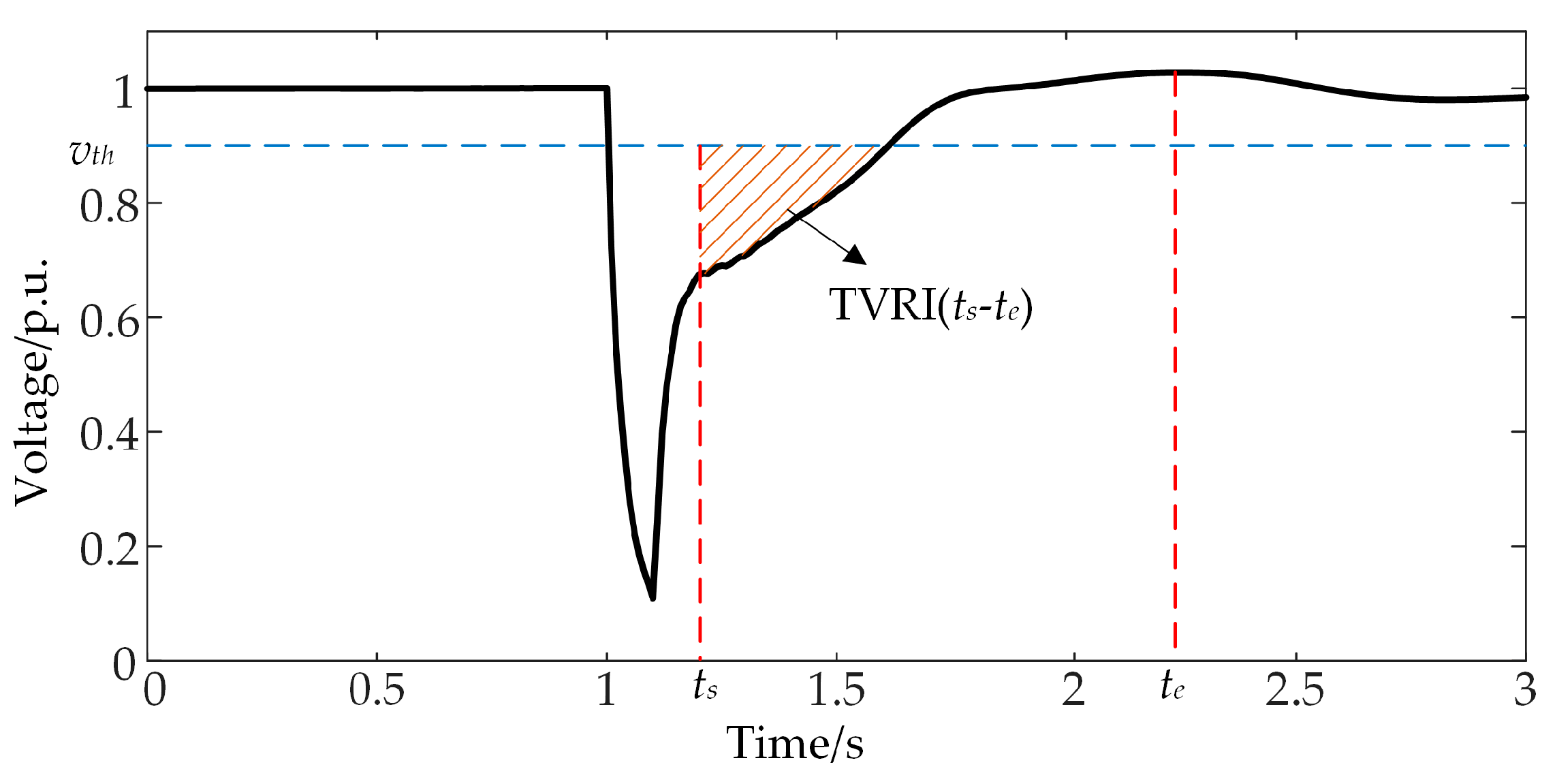
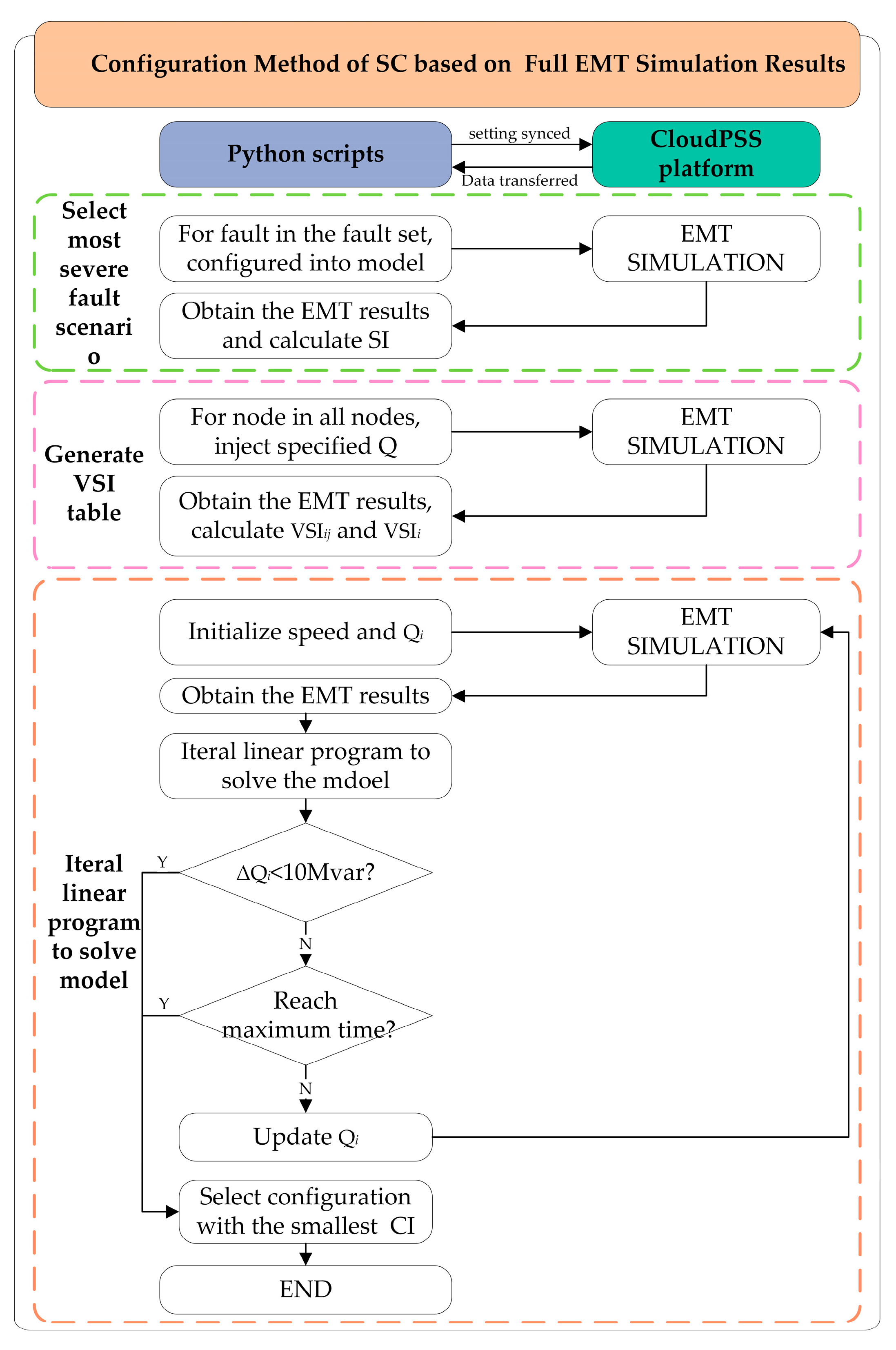
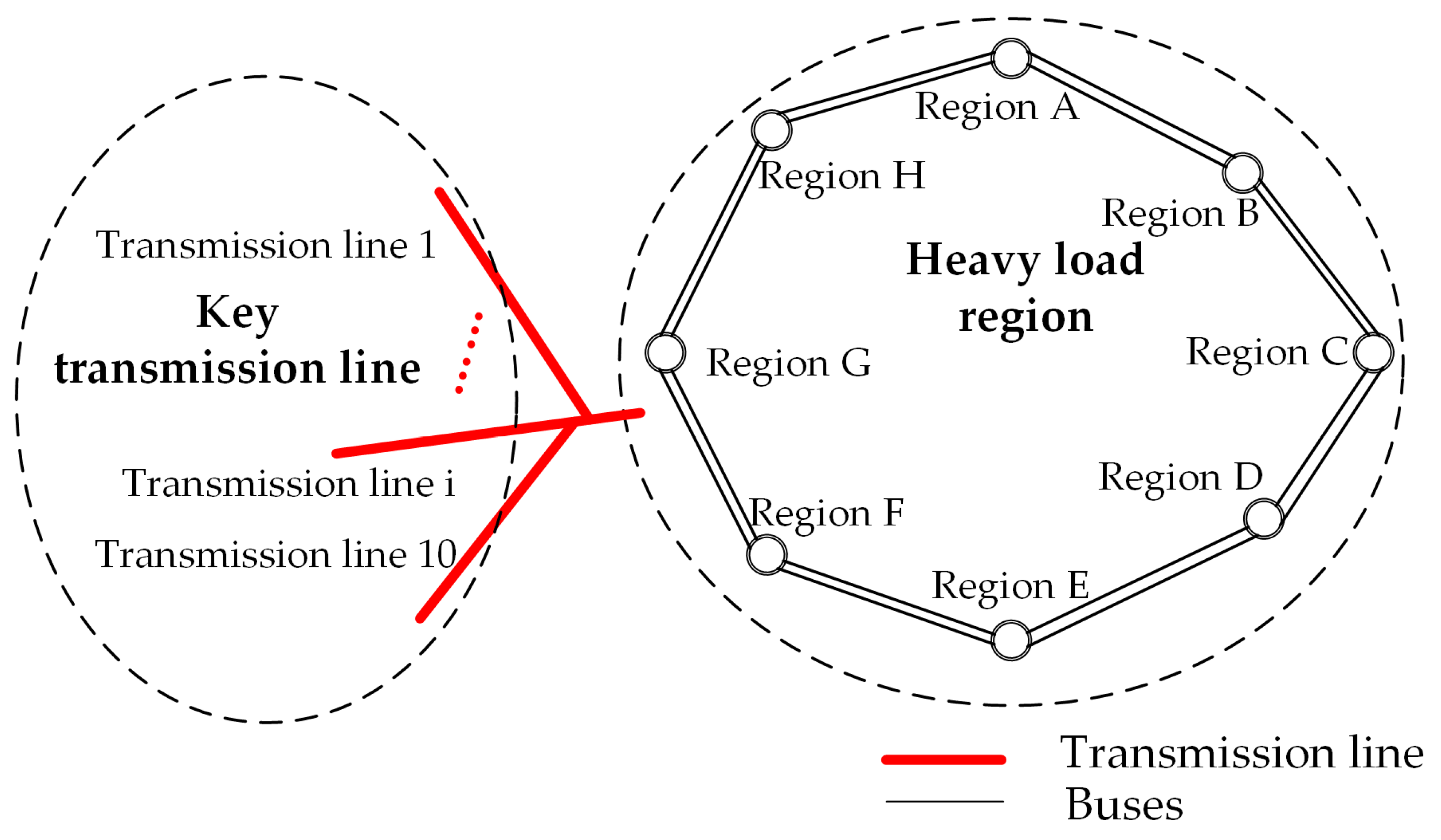
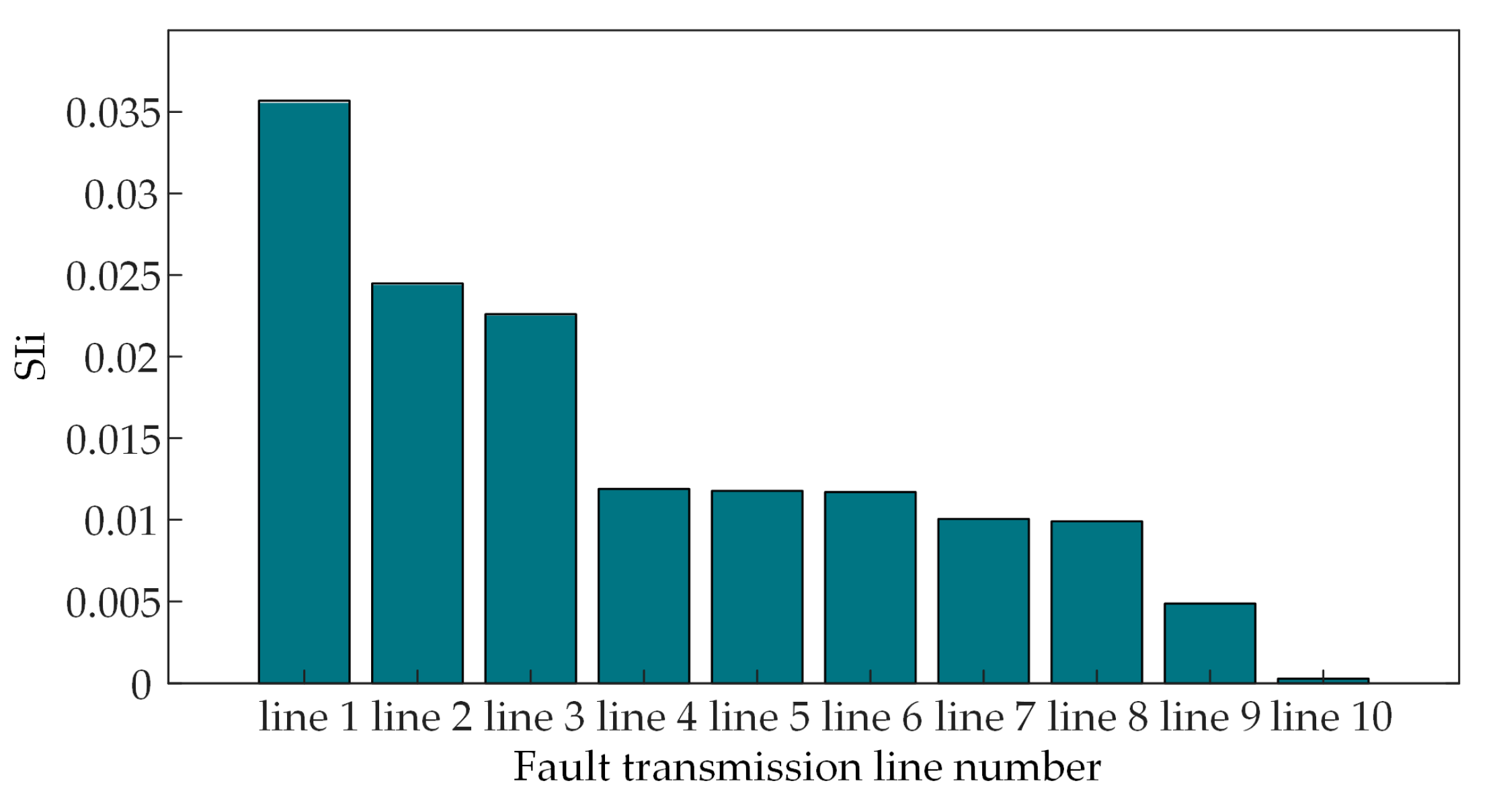
The structure of this paper is as follows: Section 2 introduces relevant indexes for evaluating transient voltage stability. Section 3 presents the optimization model for the SC configuration and solution. Section 4 describes the case study, and Section 5 concludes this paper.

2. Relevant Indexes for Evaluating Transient Voltage Stability

2.1. Severity Index

The severity index (SI) quantifies the voltage deviation severity at bus j at time t after an N-1 fault on transmission line i. The index is expressed by Equation (1):

$${{\mathit{SI}}_{\mathit{ij}}}^t=\left\{\begin{array}{l}1,R_j>25\%,t_{cl}<t<t_s\\ 1,R_j>5\%,t>t_s\\ 0,other\end{array}\right.$$

(1)

where t_cl is the fault clearing time and t_s represents 3 s after the fault begins. SI_ij^t indicates whether the voltage at bus j exceeds the limit at time t under fault scenario i as follows. If, within the time interval from t_cl to t_s, the voltage at bus j is below 0.75 p.u or above 1.25 p.u, SI_ij is incremented by 1. After t_s, if the voltage is below 0.95 p.u or above 1.05 p.u, SI_ij is again incremented by 1.

To measure the impact of fault i on all the bus voltages within the area, the observation time is discretized, and the SI_ij^t values of all buses are summed and then averaged to obtain the index, as shown in Equation (2):

$${\mathit{SI}}_i={\displaystyle \frac{1}{N}}{\displaystyle \sum _{j=1}^N(\frac{1}{T}{\displaystyle \sum _{t=t_{cl}}^T{{SI}_{\mathit{ij}}}^t})}$$

(2)

where T represents the discretized time variable and N is the number of observed buses. SI_i represents the comprehensive severity of transient voltage violations due to fault i.

2.2. Reactive Power–Voltage Sensitivity Index

The reactive power–voltage sensitivity index (VSI) characterizes the effect of injecting reactive power at node i on the transient voltage at bus j, as shown in Equation (3):

$${VSI}_{ij}={\displaystyle \frac{V_{tj}-V_{0j}}{Q_i}}j\in 0,1,2\dots \dots ni\in 0,1,2,\dots n$$

(3)

where V_tj is the steady-state voltage RMS value at bus j after time t, V_0j is the steady-state voltage RMS value at bus j before the injection of reactive power at node i, and Q_i is the reactive power injected at node i.

To quantify the effect of reactive power installation at node i on transient voltage across all buses in the area, VSI_ij is summed to obtain the index VSI_i, as shown in Equation (4):

$${VSI}_i={\displaystyle \sum _{j=0}^n{VSI}_{ij}}j\in 0,1,2\dots \dots ni\in 0,1,2,\dots n$$

(4)

where n is the total number of buses in the area, i represents the node index where reactive power compensation devices are installed, and j is the bus index. A higher VSI_i value implies greater effectiveness of reactive power compensation at bus i in improving the overall system voltage stability. Consequently, buses with a higher VSI_i are selected as candidate locations for SCs. At the same time, VSI_ij serves as heuristic information for the sizing of synchronous condensers, as detailed in Section 3 during the optimization model formulation.

2.3. Transient Voltage Instability Risk Index

When assessing the transient voltage stability, the minimum voltage and recovery time after faults are of primary concern. Both indicators indicate key information about the transient process, but the overall impact on the process of voltage recovery is not fully analyzed. Some studies use the voltage–time area of the transient voltage trajectory, referred to as the transient voltage instability risk index (TVRI), to measure this impact [19], and the definition is shown in Equation (5):

$${\mathrm{TVRI}}_i={\displaystyle {\int }_{ts}^{te}(v_{th}-v_t)*dt}\hspace{1em}if{v}_t<v_{th}$$

(5)

where vth is the lower voltage limit, v_t is the effective voltage of bus i at time t, and t_s and t_e are the start time and end time for the calculation of the TVRI_i, respectively. TVRI_i quantifies both the magnitude and duration of bus i’s voltage falling below the limit vth within the concerned period t_s to t_e, corresponding to the shaded area shown in Figure 1. A smaller TVRI_i indicates a better voltage recovery performance and higher transient voltage stability.

To calculate TVRI, discretize Equation (5) in terms of the time scale and give the overall TVRI within the whole area, as shown in Equation (6):

$$\mathrm{TVRI}={\displaystyle \sum _{i=1}^N{\displaystyle \sum _1^T(\frac{v_{it}+1+v_{it}}{2}-v_{th})*\Delta T}}\hspace{1em}if{v}_t<v_{th}i\in 1,2,\dots N$$

(6)

where T represents the discretized time variable; v_it and v_it+1 represent the voltage values of bus i at times t and t+1, respectively; ΔT represents the discrete time interval; and N represents the index of observed buses.

2.4. Comprehensive Index

When constructing the configuration optimization model, the minimum voltage is enforced as a hard constraint but excluded from the objective function. To holistically balance installed capacity and transient voltage recovery performance, a comprehensive index (CI) is proposed for the further evaluation of the optimization results, which is given by Equation (7):

$$CI={\displaystyle \sum Q}+\eta \mathrm{TVRI}$$

(7)

where Q stands for the total capacity; TVRI is given by Equation (6); and η is the impact factor of the TVRI, which is taken as 5000 in this study. A lower CI value indicates a more optimal configuration, effectively balancing both economic and technical considerations.

3. Optimizing Configuration Model Based on EMT Simulations and Solution

This study aims to ensure that the transient voltage of all buses within the heavy-load region meets the minimum requirements while achieving low configuring SC costs.

3.1. Siting Selection of SCs

To address the issue of insufficient transient reactive power support in load centers, the configuration of SCs can provide reactive power compensation at the nodes, effectively mitigating the problem of reactive power shortage after faults and improving the transient voltage stability. If the configuration scheme ensures that all the buses within the region satisfy the constraints under the most severe fault scenario, it can be considered that the transient voltage stability requirements will still be met under other fault conditions.

The primary step in optimizing the configuration of SCs is selecting appropriate connection nodes. This study begins by identifying key fault cases within the power grid and then calculating VSI_ij and VSI_i under the fault scenario. Nodes with higher VSI_i values are then selected as candidate locations. Specific steps are outlined as follows:

(1)

Conduct fault severity testing experiments based on the actual grid model: For each fault in the fault set, EMT simulations are sequentially performed. The transient voltage trajectories of all buses within the region are recorded; then, the SI under each fault scenario is calculated. The scenario exhibiting the highest SI is selected as the configuration case;

(2)

Generate a VSI table under the most severe fault scenario: In the case of the most severe scenario, EMT simulations are conducted by injecting a specified amount of reactive power at each node. The transient voltage trajectories of all nodes are observed, and VSI_ij is calculated using Equation (3); thus, the VSI table is generated;

(3)

Selecting the connection nodes: With the VSI table, VSI_i is calculated using Equation (4) to evaluate the support effect of reactive power injection at each node on the overall voltage. The top 10 nodes with the highest VSI_i values are selected as candidate sites.

3.2. Mathematical Model for SC Capacity Optimization

The objective function, aimed at minimizing the configuration cost, is presented in Equation (8):

$$f={\displaystyle \sum c}*Q_i,i\in 1,2,\dots \dots n,Q_i\in (0,Q_{\max })$$

(8)

where c represents the unit capacity cost of installing SCs, i denotes the candidate bus for installation, and Q_i is the capacity of the synchronous condenser at node i. To simplify the model, assume that the unit capacity economic cost of installing SCs is the same across all nodes. Therefore, c is set to 1, and the optimization goal reduces to minimize the total installed capacity.

Constraints of the mathematical model include power balance constraints and variable constraints:

(1) The power balance constraints are as follows:

$$\left\{\begin{array}{c}{P}_{\mathrm{g}i}-P_{\mathrm{d}i}-U_i{\displaystyle \sum _{j\in i}}{U}_j(G_{ij}\cos {\theta }_{ij}+B_{ij}\sin {\theta }_{ij})=0\\ Q_{\mathrm{g}i}-Q_{\mathrm{d}i}-U_i{\displaystyle \sum _{j\in i}}{U}_j(G_{ij}\sin {\theta }_{ij}-B_{ij}\cos {\theta }_{ij})=0\end{array}\right.$$

(9)

where P_gi, P_di, Q_gi, Q_di, and U_i represent the active power input, active power output, reactive power input, reactive power output, and voltage at node i, respectively. G_i, B_ij, and θ_ij denote the conductance, susceptance, and phase angle difference in branches i−j, respectively.

(2) The variable constraints are as follows:

$$\begin{array}{l}{VSI}_{ij}*\Delta Q_i/speed\ge \Delta V_H\\ {VSI}_{ij}*\Delta Q_i/speed\ge \Delta V_L\end{array}$$

(10)

$$S_{\min }-Q_i-1<\Delta Q_i<S_{\max }-Q_i-1i=1,2,\dots ,d$$

(11)

where ΔQ_i represents the capacity adjustment of the SC at node i and speed denotes the optimization iteration speed. ΔV_H is the deviation between the highest transient voltage and the upper limit, and ΔV_L is the deviation between the lowest transient voltage and the lower limit. As illustrated in Equation (10), the VSI_ij serves as heuristic information to guide the optimization of the capacity configuration. The underlying principle involves analyzing the transient undervoltage or overvoltage at each bus in the region, as well as the deviation between these values and their target limits. The objective is for the voltage increment at each node, after the installation of the SC, to exceed the deviation between the node voltage and its respective limit. This formulates the reactive power–voltage inequality constraints for all nodes, and ΔQ_i in each iteration is determined with VSI_ij. In Equation (11), Q_i−1 refers to the current capacity at node i, and Equation (11) restricts the variation in the SC capacity, ensuring that the total installed capacity at each node remains within the range of S_min and S_max.

Equations (8)–(11) constitute the optimization model aimed at enhancing the transient voltage at the buses within the load center area. With the goal of minimizing the total capacity, the heuristic information VSI_ij is incorporated into the constraints to guide the optimization of the variable ΔQ_i. In this model, the complex problem of transient constraints in the power grid is linearized, which facilitates its solution. Subsequently, an iterative linear optimization algorithm is employed to solve the model, thereby achieving the optimal locations and capacities of the SC.

3.3. Solutions of the Model via ILP and EMT Simulations

This study employs an iterative linear programming algorithm to solve the optimization model of SC configurations, as depicted in Figure 2. The approach of SC placement is introduced in Section 3.1, and the detailed procedure for solving the mathematical model is as follows:

• Step 1: Initialize the iteration speed, set the maximum number of iterations, and initialize the SC capacity installed at each candidate node;
• Step 2: Conduct EMT simulations and obtain voltage trajectories;
• Step 3: Based on the voltage trajectory, determine the minimum and maximum voltage values at each bus during the fault periods (0.5–3 s and 3 s after the fault starts, respectively) and solve the optimization model using linear optimization methods;
• Step 4: Obtain the capacity adjustment ΔQ. If ΔQ is less than the limit of 10 Mvar, the solution converges and proceed to Step 6. Otherwise, proceed to Step 5;
• Step 5: Check whether the iteration reaches the maximum limit. If not, substitute ΔQ into the node capacity configuration, update Qi, and repeat Steps 2 to 5. Otherwise, proceed to Step 6;
• Step 6: Analyze the iteration process and select the configuration with the smallest CI.

4. Case Study

This method is applied to the location and capacity optimization of SCs in the weak areas of the S province power grid. Within the grid, 10 typical power input transmission lines are selected for the transient voltage security study. The network topology of the load-center region is shown in Figure 3.

4.1. Process of SC Configuration in the Heavy-Load Region of S Province

The optimization study for transient voltage security in weak areas begins with analyzing the impact of key transmission line faults. Based on engineering experience, transmission lines 1–10, which supply power to the heavily loaded region, are selected for research. These lines, despite having a relatively lower priority, exhibit higher fault occurrence probabilities, and their faults directly affect transient voltage levels within the heavy-load region. They are selected to conduct N-1 three-phase-to-ground short-circuit faults separately, thereby forming the fault set. For each fault in the set, EMT simulations are performed. The transient voltage trajectories of buses in areas A-G are recorded, and the SI is calculated using Equation (2). Results are shown in Figure 4.

It is observed that scenario 1 yields the highest SI value, indicating that the N-1 three-phase-to-ground short-circuit fault on transmission line 1 has the most significant impact on the voltage stability of the whole region. As a result, this scenario is selected for further SC configuration analysis.

To conduct the analysis, set transmission line 1 to a three-phase-to-ground short-circuit fault, inject 100 Mvar of reactive power into every bus node in areas A–H, and then sequentially perform EMT simulations. With the steady-state voltage variations at all buses, the node-to-node VSI table and the node-to-region VSI_i are calculated using Equations (3) and (4). A higher VSI_i value indicates a better overall voltage enhancement at all buses with reactive power compensation at node i. To obtain the highest values, sort VSI_i and select the top 10 nodes as candidates, including Bus 185, Bus 208, Bus 51, Bus 164, Bus 232, Bus 79, Bus 133, Bus 258, Bus 112, and Bus 233, as illustrated in Figure 5.

Based on the fault scenario and candidate SC placement, the next step is to determine the optimal configuration capacity by solving the optimization model. The optimization parameters are presented in

Table 2. Optimization parameters and the fault set.

Parameter		Value
iteration speed		0.5
initial capacity/Mvar		200
voltage constraints/p.u	0.1 s–3 s	0.75
	3 s–	0.9
fault scenario		NO.1 transmission line
fault type		N-1 three-phase-to-ground short-circuit
fault start time/s		4
fault cut time/s		4.1

.

The optimal configuration scheme is obtained by solving the model, with the SC configuration process illustrated in Figure 6. Experimental results demonstrate convergence after nine EMT simulations and eight linear programming iterations.

As shown in Figure 6, all candidate nodes are initially equipped with a 200 Mvar SC. After the first EMT simulation and optimization, the capacities of Bus 185, Bus 232, and Bus 51 increase, while the capacities of other buses approach zero. After the second simulation and iteration, the capacity of Bus 185 reaches its maximum and remains unchanged, while the capacity of Bus 232 increases further. For Bus 51, the optimization suggests capacity reduction, while Bus 208 begins to increase. In the subsequent iterations, the configuration capacity of Bus 185 remains constant, and Bus 232 attains its limit and stabilizes, but Bus 208’s configuration capacity decreases to zero after the third iteration. Subsequent iterations focus on adjusting the capacity for Bus 51. After the eighth iteration and final EMT simulation, followed by another linear programming solution, the capacity change falls below 10 Mvar, satisfying the convergence condition.

This iterative process demonstrates that capacity allocation prioritizes voltage constraint satisfaction before minimizing total capacity. When selecting a configuration scheme, both cost and overall transient voltage stability should be considered. The configuration capacity, TVRI, and CI throughout the iteration process are presented in

Table 3. Index analysis during iterations.

Iteration	Capacity/Mvar	TVRI	CI	Computation Time/s
0 (Initial)	2000	1.394	8970	0.11
1	1964	0.839	6160	0.09
2	1841	1.164	7662	0.07
3	1945	1.608	9986	0.09
4	2267	0.896	6746	0.09
5	2206	0.935	6880	0.08
6	2174	0.952	6935	0.07
7	2157	0.971	7011	0.07
8	2153	0.965	6976	0.08

. Moreover, the computational time in Table 3 represents the time consumed, determined by solving the LP model at each step.

As listed in Table 3, the first iteration achieves a higher CI value, indicating superior transient stability performance. Therefore, this iteration is selected as the optimal configuration scheme, and detailed parameters are provided in

Table 4. SC configuration scheme.

Bus Index	Capacity/Mvar
Bus 185	800
Bus 51	344
Bus 232	800

.

4.2. Effectiveness Verification

4.2.1. Case 1: Configuration Under NO.1 Transmission Line Fault

To verify the effectiveness of the proposed method, a transient voltage stability analysis for all the buses within the region under the fault scenario in

Table 5. Fault scenario of case 1.

Parameter	Value
fault scenario	NO.1 transmission line
fault type	N-1 three-phase-to-ground short-circuit
fault start time/s	4
fault cut time/s	4.1
observation time/s	4–7

and the configuration scheme in Table 4 is conducted. According to the analysis, three buses, including Bus 73, Bus 65, and Bus 69, perform much worse without an SC under the fault on transmission line 1. Detailed observations focus on these buses; quantified indexes are provided in

Table 6. Transient voltage indicators of buses under the NO.1 transmission line fault.

Parameter	Bus Index	Without SC	With SC
Low transient Voltage/p.u (0.5 s after fault)	Bus 73	0.635	0.916
	Bus 65	0.638	0.916
	Bus 69	0.644	0.917
Recovery time/s (recover to 0.8 p.u)	Bus 73	4.96	4.33
	Bus 65	4.96	4.33
	Bus 69	4.95	4.33
TVRI		2.50	0.84

, and transient voltage trajectories are shown in Figure 7.

Table 6 demonstrates that the introduction of SCs significantly improves the voltage stability across various buses in the power grid. As shown in Figure 7, from 4.0 to 4.1 s, the buses are affected by the fault, causing rapid voltage drops. After the fault clearance, voltages gradually recover to pre-fault levels, between 4.1 and 5.0 s. Figure 7 also shows that after the installation of the SC, the transient voltage recovery process of the buses accelerates, and the steady-state voltage level improves. Taking Bus 73 as an example, the direction of the transient voltage trajectory change marked in the figure clearly demonstrates that the TVRI improved a lot. The time for Bus 37 to recover to 0.8 p.u decreased from 4.96 s to 4.33 s. Additionally, 0.5 s after the fault, the minimum voltage at that time increased from 0.635 p.u to 0.916 p.u. Similarly, transient voltage behaviors for Buses 65 and 69 are observed in Table 6 and Figure 7. The analysis above indicates that the installation of SCs makes the buses recover in a shorter time, reducing the risk of further faults and ensuring the safe and stable operation of the power system. Furthermore, by analyzing the TVRI of the heavily loaded region, it is found that under fault scenario 1, the equipped SC has reduced the system’s overall TVRI value from 2.5 to 0.84, achieving a decrease of approximately 66%. The comprehensive transient voltage stability in the region have been enhanced.

To further observe the overall improvement of the voltage within the region, the top 20 buses most severely affected by the fault without SC installation are selected. The heatmap in Figure 8 demonstrates the transient voltage variation during 0.5–1 s after the fault. From the left heatmap, it is apparent that, without SCs, the overall transient voltage across the buses ranges from 0.7 to 0.85 p.u. It can be seen on the right side that, with SCs configured, the transient voltage has improved markedly, with all buses recovering to approximately 1.0 p.u over 0.5–1 s. In general, the proposed scheme not only provides support for transient voltage but also significantly accelerates voltage recovery. The above analysis focuses on the buses most affected by the fault before the installation of SCs. Subsequently, buses exhibiting low transient voltage levels post-SC installation are analyzed. EMT simulation results are analyzed, and buses with the lowest voltages and slowest recovery times are identified, namely Bus 35, Bus 33, and Bus 36, as shown in

Table 7. Transient stability of buses with SCs.

Bus Index	Low Voltage/p.u	Recovery Time/s
Bus 35	0.779	4.56
Bus 33	0.781	4.55
Bus 36	0.783	4.55

.

Indicators in Table 7 reveal that within 0.5–1 s after the fault, the lowest voltage in the load-center region is 0.779 p.u, which exceeds the minimum transient voltage threshold (0.75 p.u). The time taken for the voltage to recover to 0.8 p.u is 4.56 s, indicating satisfactory recovery performance. Overall, buses within the heavy-load center satisfy the transient voltage stability requirements with SCs.

4.2.2. Case 2: Configuration Under NO.2 Transmission Line Fault

To further verify the effectiveness of the proposed scheme, the transmission line 2 fault scenario, with the second highest SI value as shown in Figure 4, is chosen to conduct EMT simulations with the configuration in Table 4. The fault parameters are defined in

Table 8. Fault scenario of case 2.

Parameter	Value
fault scenario	NO.2 transmission line
fault type	N-1 three-phase-to-ground short-circuit
fault start time/s	4
fault cut time/s	4.1
observation time/s	4–7

. Simulation results reveal that buses with insufficient voltage support before the configuration include Buses 73, 65, and 75, and their indicators are depicted in

Table 9. Transient voltage indicators of buses under the NO.2 transmission line fault.

Parameter	Bus Index	Without SC	With SC
Low transient voltage/p.u (0.5 s after fault)	Bus 73	0.785	0.972
	Bus 65	0.787	0.972
	Bus 75	0.790	0.973
Recovery time/s (recover to 0.8 p.u)	Bus 73	4.54	4.27
	Bus 65	4.53	4.27
	Bus 75	4.53	4.27
TVRI		1.557	0.762

, and transient voltage trajectories are shown in Figure 9.

The transient voltage trajectories of buses in the heavy-load area caused by the fault on transmission line 2 are shown in Table 9. The overall TVRI value within the region during the fault is 1.557, significantly lower than the TVRI of 2.5 under the fault on transmission line 1. It indicates that the fault on transmission line 2 is less severe than that on transmission line 1, which confirms the severity ranking shown in Figure 4. The direction of the voltage trajectory change, as marked in Figure 9, indicates that the three buses, which are significantly impacted by the fault, show a substantial reduction in the voltage-time area after configuring SCs. Figure 9 demonstrates that the time for Bus 73 to recover to 0.8 p.u under the fault is reduced from 4.54 s to 4.27 s due to the installation. Additionally, 0.5 s after the fault, the lowest voltage at that moment increases from 0.785 p.u to 0.972 p.u with the SC configuration. Similarly, Buses 65 and 75 show similar improvements in both transient voltage support and recovery time under the influence of the SC. The above shows that the proposed configuration still can support the transient voltage recovery under the NO.2 transmission line fault. The installation of SCs accelerates transient voltage recovery in buses, reduces overvoltage during the process, and improves the steady-state voltage level. Also, the overall system TVRI value decreases from 1.557 to 0.762, improving the overall voltage stability by approximately 51% and enhancing regional voltage stability.

Figure 10 demonstrates the voltage heatmap of the top 20 buses most severely affected by the NO.2 transmission line fault before the installation, with observations 0.5–1 s post-fault. The left heatmap shows that without SCs, the overall voltage recovers to approximately 0.8–0.95 p.u, while all bus voltages with SCs recover to around 1 p.u within 0.5 s, as shown in the right heatmap. As a consequence, the proposed configuration shows strong voltage stability support under the fault as well.

Table 10. Transient stability of buses with SC under the NO.2 transmission line fault.

Bus Index	Low Voltage/p.u	Recovery Time/s
Bus 35	0.938	4.34
Bus 33	0.939	4.34
Bus 36	0.939	4.33

presents the transient voltage indicators for buses with relatively low transient voltage levels in the region after SC installation, including Bus 35, Bus 33, and Bus 36. Within 0.5–1 s after the fault, the three lowest bus voltages in the load area are around 0.938 p.u, and the time for the voltages recovering to 0.8 p.u is around 4.34 s, showing excellent transient voltage performance.

4.2.3. Case 3: Configuration Under a Severe External Fault

In addition to examining the transmission lines directly supplying power to the region, a transmission line from outside the region that significantly impacts the system is also studied. Although the fault impact of this external transmission line is substantial, it holds a lower priority and has a relatively low probability of occurrence. Full EMT simulations are conducted both without and with the SC configuration shown in Table 4, and the fault setting parameters are shown in

Table 11. Fault scenario of case 3.

Parameter	Value
fault scenario	A transmission line from outside the region
fault type	N-1 three-phase-to-ground short-circuit
fault start time/s	4
fault cut time/s	4.1
observation time/s	4–7

. Simulation results show that before installing the SC, Buses 73, 65, and 69 exhibited lower voltage levels compared to other buses. The transient indicators and voltage trajectories of these buses are shown in

Table 12. Transient voltage indicators of buses under a severe external fault.

Parameter	Bus Index	Without SC	With SC
Low transient voltage/p.u (0.5 s after fault)	Bus 73	0.550	0.719
	Bus 65	0.553	0.722
	Bus 69	0.559	0.729
Recovery time/s (recover to 0.8 p.u)		0.7 p.u	0.8 p.u
	Bus 73	5.46	4.7
	Bus 65	5.39	4.7
	Bus 69	5.27	4.68
TVRI		5.111	1.368

and Figure 11 separately.

Under this fault scenario, the overall TVRI reaches 5.111, which exceeds 2.5, indicating higher transient severity. Figure 11 shows that, without the SC configuration, the steady-state voltage of the three buses does not recover to its original value in this case. However, with the SC configuration, the transient voltages of the buses recover to pre-fault levels. For Buses 73, 65, and 69, without the SC configuration, the voltages recover to 0.7 p.u in around 5.3 to 5.4 s and stabilize at that level. With the SC, these buses recover to 0.8 p.u approximately 0.7 s after the fault. Additionally, 0.5 s after the fault, the minimum voltage of the three buses rises from around 0.55–0.6 p.u to approximately 0.72 p.u, demonstrating a significant improvement in transient voltage support.

Under fault case 3, the configuration of SC reduces the overall system TVRI value from 5.111 to 1.368, improving by 73%. Therefore, the transient voltage stability in the heavy-load center shows considerable enhancement.

Figure 12 demonstrates the voltage heatmap of the top 20 most affected buses under the fault without SC installation, observed 0.5–1 s after the fault. The heatmap shows that the overall voltage ranges between 0.6 and 0.7 p.u without the SC, while all bus voltages recover to around 0.95 p.u within 1 s with the SC. As observed, the scheme also demonstrates robust voltage stability support in this case.

4.3. Impact of Parameters in the Algorithm on the Optimization Results

In the process of locating and sizing SCs via the iterative linear optimization algorithm, parameter selection may significantly affect the final configuration. This section evaluates the impacts of iteration speed and constraint settings on SC deployment schemes.

4.3.1. Impact of Iteration Speed on the Scheme

To study the impact of different iteration speeds on the SC configuration scheme, the speed is set to 0.2, 0.5, 0.7, 1, and 1.5, respectively, with the NO.1 transmission line fault, as shown in Table 5. The optimization model is solved by combining the EMT simulations with these iteration speeds. Figure 13 and

Table 13. Transient indicators of schemes under different iteration speeds.

Speed	Number of Iterations	Capacity/Mvar	Configuration Scheme/Mvar		TVRI	CI
1.5	18	2119	Bus 185	800	0.776	5998
			Bus 51	519
			Bus 232	800
1.0	3	2143	Bus 185	800	0.974	7011
			Bus 51	542
			Bus 232	800
0.5	9	1964	Bus 185	800	0.839	6160
			Bus 51	800
			Bus 232	344
0.7	16	2092	Bus 185	800	0.831	6250
			Bus 51	492
			Bus 232	800
0.2	16	1941	Bus 185	800	0.828	6081
			Bus 51	341
			Bus 232	800

present the configuration schemes of the SC obtained under different iteration speeds and provide the number of iterations, total capacity, specific configuration schemes, and the overall TVRI and CI.

When the iteration speed is set to 1.5, the solution process converges after 18 iterations, with a total capacity of 2119 Mvar, a TVRI of 0.776, and a CI of 5998. This configuration achieves optimal transient stability enhancement with reasonable capacity allocation; however, excessive iterations (18 cycles) incur high computational costs.

When the iteration speed is 1.0, the solution converges after just three iterations. However, this configuration scheme takes the highest total capacity of 2143 Mvar but results in the poorest TVRI of 0.974. For speeds of 0.7 and 0.2, the results for the number of iterations, fixed capacity, and the overall effect are quite similar. Both configurations require 16 iterations, leading to higher computational resource consumption.

When the speed is set to 0.5, the configured capacity is lower, and the solution converges after only nine iterations. Both the TVRI of 0.839 and the CI of 6160 are satisfactory. A comparison between the solution processes for speeds of 0.2 and 0.5 reveals that, with a speed of 0.2, the search is slower but more refined, leading to better results in terms of transient effects and capacity configuration. However, the scheme obtained at speed 0.2 differs by only 1.28% in the overall CI and 1.17% in the configuration capacity compared to that obtained at a speed of 0.5, but seven more iterations consume more computational resources and solving time. Therefore, setting the speed to 0.5 offers a better balance between computational resources and the overall performance of the configuration scheme.

The above analysis demonstrates that iteration speed affects the number of iterations, which in turn influences search precision and the overall performance. The total computation time is primarily determined by both the EMT simulation time and the optimization problem-solving time. EMT simulations are computationally intensive. For instance, a 10 s simulation requires approximately 20 min on the computational platform. However, the optimization-solving process takes less than 0.2 s, as shown in Table 3. As a result, higher iteration counts lead to longer optimization durations. When speeds are set to 0.2, 0.7, and 1.5, the number of iterations is high, resulting in more iterations but achieving favorable CI values. Conversely, when the speed is set to one, the model converges in only three iterations, which takes fewer solving steps and computation resources, but the overall performance is not as good.

In addition, simulation results in Table 13 show that increasing the capacity of SCs at nodes does not necessarily lead to a better overall transient voltage improvement. For instance, compared to the iteration speed of 0.7, the configuration scheme obtained with the speed of 0.2 requires a configuration capacity of 1941 Mvar, which is less than the 2092 Mvar required at a speed of 0.7. However, the overall TVRI for the scheme at speed 0.2 is 0.828, which is slightly better than the 0.831 achieved at speed 0.7. Therefore, optimal capacity allocation, rather than maximal capacity, can not only reduce costs but also enhance the system’s transient voltage stability more effectively.

4.3.2. Impact of Constraints on the Scheme

To evaluate the impact of constraints on the configuration, the minimum voltage threshold between 0.5 and 3 s after the fault is set to 0.75 p.u and 0.8 p.u under the NO.1 transmission line fault; parameters are shown in Table 5. Through EMT simulations and linear programming, configuration schemes with optimal CI are selected. The impact of different constraints on the total capacity, TVRI, and CI is analyzed, as shown in

Table 14. Impact of constraints on the configuration.

Constraints/p.u	Speed	Iterations	Capacity/Mvar	TVRI	CI
0.75	0.5	9	1964	0.839	6160
	1	3	2143	0.974	7011
0.8	0.5	20	2780	0.643	5994
	1	4	3077	0.714	6645

and Figure 14.

First, the impact of constraints on the number of iterations is analyzed. With an iteration speed of 0.5, the process requires nine and twenty iterations for transient voltage constraints of 0.75 and 0.8, respectively. At the iteration speed of one, the iteration counts are three and four for under the same constraints. This indicates that higher transient voltage constraints lead to more iterations and, consequently, greater computational resources.

Next, the effect of constraint conditions on the configuration scheme is analyzed. At an iteration speed of 0.5, the total configuration capacity required for transient voltage constraints of 0.75 p.u and 0.8 p.u are 1964 Mvar and 2780 Mvar, respectively. When the iteration speed is set to one, the corresponding values are 2143 Mvar and 3077 Mvar. This indicates that higher transient voltage constraints require larger configuration capacities, which, in turn, lead to increased costs.

Additionally, the impact of constraint conditions on TVRI is analyzed. With an iteration speed of 0.5, the regional TVRI values for transient voltage constraints of 0.75 p.u and 0.8 p.u are 0.938 and 0.643, respectively. With an iteration speed of one, the TVRI values are 0.974 and 0.714. This indicates that higher transient voltage constraints result in a greater improvement in the TVRI of the region, demonstrating enhanced transient voltage support.

Considering the combined effects of constraint conditions on configuration capacity and TVRI, the 0.5-speed configuration under the 0.8 p.u constraint requires 2780 Mvar (vs. 3077 Mvar at 1.0 speed) while achieving a lower TVRI (0.643 vs. 0.714). This also indicates that properly placing the SC at nodes can effectively enhance the support provided by the SC while keeping costs low.

Finally, the impact of constraint conditions on the CI is further analyzed. With an iteration speed of 0.5, the CI values for transient voltage constraints of 0.75 p.u and 0.8 p.u are 6160 and 5994, respectively. With an iteration speed of one, the corresponding CI values are 7011 and 6645. These results show that stricter voltage constraints balance better economic costs with technical effectiveness.

All in all, Table 14 shows that when the voltage constraint increases from 0.75 p.u to 0.8 p.u, the obtained configuration scheme improves the overall TVRI significantly but requires more capacity and incurs higher cost. Meanwhile, the configuration after the constraint increase has a lower CI, achieving a better cost–performance balance. Therefore, when the proposed method is applied in practical engineering, voltage constraints should be selected properly to achieve the desired configuration effect.

Apart from this, it can be observed that at an iteration speed of 0.5 increases the constraint requirement and results in more iterations and computational resources, which means the problem-solving process becomes more complex. Higher transient voltage constraint demands impose stricter demands on the grid’s security, necessitating the consideration of more complex transient dynamics within the system, further emphasizing the advantages of using time-domain simulation data to obtain the SC configuration.

5. Conclusions

Based on the analysis above, the contribution of this work can be concluded as follows:

• This paper proposes a configuration method for SCs driven by full EMT simulation, where transient voltage support is directly used as a constraint to guide the configuration, ensuring the transient stability of the heavy-load area with minimized costs;
• SI is introduced to measure the overall impact of faults on voltage in heavily loaded areas. Through EMT simulation and SI calculation, the most severe fault scenario, the fault on NO.1 transmission line 1, is identified;
• The VSI indicator is introduced, and full EMT simulations are conducted to calculate the VSI for nodes within the region. The top 10 nodes with the highest VSI are considered as candidate nodes for the configuration of SCs;
• The proposed configuration method demonstrates excellent convergence and saves computational resources, making it applicable for practical engineering applications. Under the most severe fault scenario, the configuration ensures that the transient voltage at all buses in the region satisfies the requirement with low cost. The transient voltage, recovery time, and overall TVRI all improve a lot. The configuration scheme is validated under other fault scenarios too;
• A higher iteration speed might lead to slower convergence and more iterations, but it yields better performance. It is concluded that setting the iteration speed to 0.5 strikes a balance between computational resources and overall performance;
• The stricter limit-exceeding indicators make the solution process more complex and demand more computational resources. The appropriate safety indicators should be selected for engineering applications;
• The proposed method is not only suitable for the configuration of SC but also for the configuration of other VAR compensator devices.

Although this study has completed the above work, there are still shortcomings. On the one hand, the optimization model does not consider factors such as the configuration and maintenance costs of the SC in detail. On the other hand, the fault set selection is based on engineering experience and constrained by computational resources. Hence, future research should prioritize refining economic analysis through dynamic modeling frameworks that incorporate SC life-cycle costs (installation, maintenance, and decommissioning) and market-driven revenues such as reactive power ancillary services. Additionally, intelligent fault set generation methods leveraging machine learning could be developed to automatically prioritize critical contingencies, achieving an optimal balance between computational efficiency and scenario completeness for practical grid applications.

References

1. Guo, Q.; Li, Z. Summarization of Synchronous Condenser Development. Proc. CSEE 2023, 43, 6050–6064. [Google Scholar]
2. Gan, W.; Chen, D.; Cui, T. Research on Configuration of Distributed Synchronous Condenser in UHV AC/DC Hybrid Power Grid. Hunan Electr. Power 2022, 42, 35–42, 72. [Google Scholar]
3. Chang, H.; Huo, C.; Liu, F. Research on Optimal Allocation Method of Synchronous Condensers for Improving Transient Voltage Stability Level of Weak Sending-End Power Grid. Power Syst. Prot. Control 2019, 6, 90–95. [Google Scholar]
4. Li, Z.; Jiang, W.; Wang, Y. Key Technical Parameters and Optimal Design of New Types of Large Capacity Synchronous Condenser. Large Electr. Mach. Hydr. Turb. 2017, 4, 15–22. [Google Scholar]
5. Zhang, J.; Meng, F.; Wu, L. Research on Distributed Condenser Capacity Configuration of New Energy Field Station Based on the Weighted Proportion of Electrical Parameters Index. Power Syst. Technol. 2024, 48, 4185–4195. [Google Scholar]
6. Wang, Z.; Liu, M.; Li, H. Optimal Configuration Method of Synchronous Condenser to Improve the Delivery Capacity of New Energy Cluster in Weak Grid. Electr. Power Autom. Equip. 2024, 44, 30–36, 44. [Google Scholar]
7. Zhou, Y.; Sun, H.; Xu, S. Synchronous Condenser Optimized Configuration Scheme for Power Grid Voltage Strength Improvement. Power Syst. Technol. 2022, 46, 3848–3856. [Google Scholar]
8. Liu, C.; Xu, D.; Wu, C. Location and Sizing Strategy of Distributed Condensers Considering Frequency Stability Constraints. Electr. Power Constr. 2023, 44, 106–114. [Google Scholar]
9. Zhao, B.; Hu, Z.; Song, Y. Optimal Planning of Quasi Synchronous Condenser for Power Transmission System with Infeed HVDC. Power Syst. Technol. 2019, 43, 1151–1162. [Google Scholar]
10. Richard, R.L.; Masood, N.A.; Saha, T.K. Optimal Allocation of Synchronous Condensers in Wind Dominated Power Grids. IEEE Access 2020, 8, 45400–45410. [Google Scholar] [CrossRef]
11. Suo, Z.; Li, H.; Zhang, F. Optimal Configuration of a Distributed Synchronous Condenser for an HVDC Sending-End System with a High Proportion of Renewable Energy. Power Syst. Prot. Control 2022, 50, 133–141. [Google Scholar]
12. Yang, J.; Shi, Z.; He, C. Optimal Configuration Strategy of Condenser for Improving Short-Term Voltage Safety in a Sending-End Power Grid with a High Renewable Penetration Level. J. Shandong Univ. (Eng. Ed.) 2024, 54, 174–182. [Google Scholar]
13. Shen, G.; Guo, J.; Chang, J. Optimal Site Selection Algorithm of Synchronous Condensers in Renewable Energy Resources Bases Considering Synchronization Stability. Comput. Simul. 2024, 41, 94–101. [Google Scholar]
14. Hadavi, S.; Mansour, M.Z.; Bahrani, B. Optimal Allocation and Sizing of Synchronous Condensers in Weak Grids with Increased Penetration of Wind and Solar Farms. IEEE J. Emerg. Sel. Top. Circuits Syst. 2021, 11, 199–209. [Google Scholar] [CrossRef]
15. Jian, W.; Zhou, Z.; Tang, F. Optimal Configuration of Synchronous Condensers for Suppressing Multi-infeed DC Commutation Failure. High Volt. Technol. 2021, 47, 169–177. [Google Scholar]
16. Wang, Q.; Li, T.; Tang, X. Method of Site Selection for Synchronous Condenser Responding to Commutation Failures of Multi-infeed DC System. Autom. Electr. Power Syst. 2019, 43, 222–227. [Google Scholar]
17. Hadavi, S.; Saunderson, J.; Mehrizi-Sani, A. A Planning Method for Synchronous Condensers in Weak Grids Using Semi-Definite Optimization. IEEE Trans. Power Syst. 2023, 38, 1632–1641. [Google Scholar] [CrossRef]
18. Paramasivam, M.; Salloum, A.; Ajjarapu, V. Dynamic Optimization Based Reactive Power Planning to Mitigate Slow Voltage Recovery and Short-Term Voltage Instability. IEEE Trans. Power Syst. 2013, 28, 3865–3873. [Google Scholar] [CrossRef]
19. Zhou, S.; Tang, F.; Liu, D. A Dynamic VAR Optimal Configuration Method for Reducing the Risk of Transient Voltage Instability. Power Syst. Prot. Control 2018, 46, 68–75. [Google Scholar]
Figure 1. Illustration of TVRI.
Electronics 14 01243 g001
Figure 2. Configuration method of an SC.
Electronics 14 01243 g002
Figure 3. Network topology of the S province heavy-load center.
Electronics 14 01243 g003
Figure 4. SIi under transmission line faults.
Electronics 14 01243 g004
Figure 5. Top 10 VSI nodes.
Electronics 14 01243 g005
Figure 6. Node capacity configuration process.
Electronics 14 01243 g006
Figure 7. Voltage trajectories of buses without and with SCs.
Electronics 14 01243 g007
Figure 8. Voltage heatmap of key buses (after fault 0.5–1 s).
Electronics 14 01243 g008
Figure 9. Voltage trajectories of buses under the NO.2 transmission line fault without and with SCs.
Electronics 14 01243 g009
Figure 10. Voltage heatmap of key buses under NO.2 transmission line (after fault 0.5–1 s).
Electronics 14 01243 g010
Figure 11. Voltage trajectories of buses under a severe external fault.
Electronics 14 01243 g011
Figure 12. Voltage heatmap of key buses under a severe external fault (after fault 0.5–1 s).
Electronics 14 01243 g012
Figure 13. Impact of iteration speed on the scheme.
Electronics 14 01243 g013
Figure 14. Surface plot of the impact of constraints on the configuration.
Electronics 14 01243 g014