Application of Deep Dilated Convolutional Neural Network for Non-Flat Rough Surface

Abstract

In this paper, we propose a novel deep dilated convolutional neural network (DDCNN) architecture to reconstruct periodic rough surfaces, including their periodic length, dielectric constant, and shape. Historically, rough surface problems were addressed through optimization algorithms. However, these algorithms are computationally intensive, making the process very time-consuming. To resolve this issue, we provide measured scattered fields as training data for the DDCNN to reconstruct the periodic length, dielectric constant, and shape. The numerical results demonstrate that DDCNN can accurately reconstruct rough surface images under high noise levels. In addition, we also discuss the impacts of the periodic length and dielectric constant of the rough surface on the shape reconstruction. Notably, our method achieves excellent reconstruction results compared to DCNN even when the period and dielectric coefficient are unknown. Finally, it is worth mentioning that the trained network model completes the reconstruction process in less than one second, realizing efficient real-time imaging.

1. Introduction

Electromagnetic imaging is an advanced and promising technology that utilizes the emission of electromagnetic waves to illuminate objects within a specified area of interest. By sending these waves into the environment, the system captures the scattered field information that is produced when the electromagnetic waves interact with various materials. These scattered data are subsequently processed to reconstruct crucial details about the object being examined, including its position, shape, and material composition. This innovative imaging technique is increasingly applied across a diverse range of fields. For instance, in surface inspection, it aids in identifying flaws or irregularities in industrial components. In biomedical imaging, it provides insights into the internal structures of biological tissues, enabling better diagnostics and treatment planning. Similarly, in non-destructive testing, it allows the evaluation of materials without causing any harm, ensuring integrity and safety in various applications. Despite its wide applicability, electromagnetic imaging still encounters significant challenges that can complicate the reconstruction process. Key issues include (1) poor penetration, (2) ill-posedness, (3) nonlinearity, (4) curse of dimensionality, (5) calculation problems of optimization programs; (6) parameter selection problems [1,2,3,4]. However, achieving a high-quality reconstructed image remains a complex endeavor due to the inherent difficulties associated with the aforementioned challenges. In order to overcome them, electromagnetic imaging processes often involve converting the inverse scattering problem into an optimization problem and solving it using iterative algorithms. Unfortunately, though the iterative algorithm is able to gain reconstruction results, it is very time-consuming and computationally intensive. This paper utilizes dilated convolution within the convolutional layers, a technique that enhances standard convolution by incorporating gaps or “holes” into the filter. This approach effectively augments the receptive field without imposing additional computational burdens, preserving the intrinsic benefits of conventional convolutions. According to the above discussion, traditional algorithms are time-consuming and computationally intensive, making real-time imaging challenging. However, most studies have shown that the shortcomings of traditional algorithms can be improved through artificial intelligence technology.

Electromagnetic imaging of rough surfaces has been approached through two primary categories: conventional algorithms [1,2,3,4,5,6,7,8,9] and artificial intelligence techniques [10,11]. Conventional algorithms such as the gradient method, Particle Swarm Optimization (PSO) and Self-Adaptive Dynamic Differential Evolution (SADDE) [4], which have long been the foundation of electromagnetic imaging, typically rely on intricate mathematical models and iterative procedures. These methods are well-established and dependable but often time-intensive and computationally demanding. In fast-paced research environments and practical applications, such limitations pose challenges, as timely imaging results are crucial for efficient data interpretation and decision-making. In recent years, some researchers are still working on improving and optimizing traditional algorithms to handle the complexity of non-underlying surfaces more effectively. In 2004, Shenawee proposed a fast-forward solver based on the Steepest Descent Fast Multipole Method (SDFMM) combined with Fletcher and Powell search techniques to reconstruct the random rough surface. Numerical results indicated a significant enhancement in surface profile reconstruction by using a multi-frequency strategy. Additionally, by implementing the multi-incidence strategy, we could further improve contour reconstruction, even when applied at a single frequency [1]. In 2007, Firoozabadi used the Levenberg–Marquardt algorithm for microwave-based subsurface sensing of lossy dielectric objects embedded in lossy ground with unknown rough surfaces. Numerical results showed that buried objects were successfully located and their size and shape characterization was sufficiently accurate [2]. In 2018, Chen introduced an iterated marching method for reconstructing rough, perfectly reflective one-dimensional surfaces. The numerical results indicated that this approach yielded a reconstructed surface profile that closely matched the exact shape and demonstrated strong stability [3]. In the same year, Chiu used SADDE to reconstruct the shape of rough surfaces. Numerical simulations showed that the proposed method could successfully reconstruct the period length, relative permittivity, and shape of different surfaces [4]. In 2020, the Finite Element Method (FEM) and Boundary Integral Method (BIM) were proposed to reconstruct a two-dimensional coated object embedded in a one-dimensional dielectric rough surface successfully [5]. In 2021, Sefer developed a method to reconstruct the surface in an iterative manner through integral equations and data equations. Numerical analysis showed that the proposed method achieved good reconstruction, demonstrating its effectiveness in accurately capturing surface features [6]. In 2022, Sefer utilized Newton’s iteration method to reconstruct the rough surface profile while taking Impedance Boundary Conditions (IBCs) into account. Numerical results indicated that this approach yielded highly satisfactory outcomes for moderately rough surface profiles, particularly when the roughness deviation is about half the wavelength [7]. In 2023, Özdemir introduced Multiplicative Regularized Contrast Source Imaging as a technique for reconstructing objects in bilayer media with uneven interfaces. Numerical simulations demonstrated that this new method greatly reduced computation time compared to conventional techniques while maintaining the same level of accuracy [8]. In 2024, Sefer employed single-frequency Reverse Time Migration (RTM) techniques to accurately reconstruct two-dimensional rough surface profiles. Numerical simulations indicated that this method produced robust reconstructions even under high noise conditions. However, this approach required a substantial number of sources and measurements, resulting in a considerable computational burden [9].

Given the rapid advancement of artificial intelligence technologies, their applications have expanded across various domains, including the analysis and manipulation of non-flat surfaces. This integration has proven to be instrumental in addressing complex challenges in fields such as computational geometry, computer graphics, and materials science. In 2022, Aydin introduced a deep learning approach utilizing Convolutional Neural Networks (CNNs) to reconstruct rough surfaces. Numerical evaluations demonstrated that this method achieved effective surface reconstruction. However, this technique was only workable under predetermined dielectric constant and [10]. In the same year, he applied CNN-based deep learning architecture to reconstruct the impenetrable rough surfaces [11].

In the context of ongoing research, there is a scarcity of studies focused on the application of artificial intelligence to non-planar rough surfaces. This paper introduces several key innovations:

• We present a DDCNN architecture designed for the reconstruction of periodic non-flattened surfaces. Notably, this approach is able to reconstruct the period, permittivity and shape of the rough surface simultaneously.
• Our numerical simulations demonstrate the robustness and precision of the proposed DDCNN architecture across varying noise conditions.
• The findings of this study highlight the pivotal role of AI in the reconstruction of surface coefficients. We delineate a hierarchy of reconstruction priorities during the training process: the primary focus is on achieving a surface period, followed by the secondary goal of estimating the dielectric constant, with the shape factor representing the final target. This prioritization arises from the varying sensitivities of each coefficient to the scattered field data, indicating an intricate interplay between these parameters in the reconstruction process.

Section 2 presents the formula and theory for non-flat rough surface. DDCNN architecture is presented in Section 3. Section 4 gives the numerical results. Section 5 provides the conclusions.

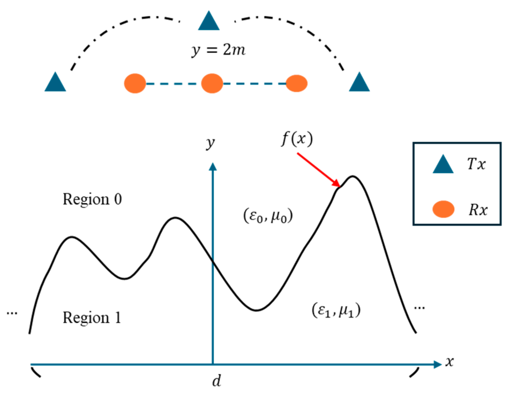
2. Formula and Theory

In this paper, we analyze a two-dimensional scenario involving periodic rough surfaces, as illustrated in Figure 1. The configuration comprises upper and lower dielectric half-spaces, separated by a rough interface defined by the function $f\left(x\right)$. This rough surface exhibits periodicity with a periodic length of d in the x-direction and a height of $y=f\left(x\right)$ in the y-direction. In regions 0 and 1, the respective permittivities and permeabilities are $({\epsilon }_0,{\mu }_0)$ and $\left({\epsilon }_1,{\mu }_1\right)$. The periodic rough surface extends infinitely in the z-direction, meaning its characteristics vary solely along the x and y axes. We then consider a uniform incident plane wave described by the time-harmonic expression $e^{j\omega t}$, propagating parallel to the z-axis, which classifies it as a transverse magnetic (TM) polarized wave $({\displaystyle \frac{\partial }{\partial z}}=0)$. The electric field associated with an incident wave ${\stackrel{⃑}{E}}_i$ approaching at an angle $\mathrm{\varnothing }$ is given by the following equation.

$${\stackrel{⃑}{E}}_i\left(x,y\right)=e^{-j{k}_0(x·sin\mathrm{\varnothing }-y·cos\mathrm{\varnothing })}\widehat{z},k_0=\omega \sqrt{{\epsilon }_0{\mu }_0}$$

(1)

The electromagnetic field is governed by Maxwell’s equations. To compute the scattered electric field at any point in the upper region, we employ a two-dimensional periodic Green’s function. The scattered field can be expressed in integral representation of the surface field by using Green’s theory in the upper region [4,12,13]:

$$E_s\left(x,y\right)={\int }_{-d/2}^{d/2}\left[{\displaystyle \frac{\partial G_0\left(x,y;x^{\prime },f\left(x^{\prime }\right)\right)}{\partial n^{\prime }}}{·E}_0\left(x^{\prime },f\left(x^{\prime }\right)\right)-G_0\left(x,y;x^{\prime },f\left(x^{\prime }\right)\right)·{\displaystyle \frac{\partial E_0\left(x^{\prime },f\left(x^{\prime }\right)\right)}{\partial n^{\prime }}}\right]\sqrt{1+{\left(f^{\prime }\right(x^{\prime }\left)\right)}^2}d{x}^{\prime }, for y>f\left(x\right)$$

(2)

where $E_0$ represents the electric field on the upper surface, and $n^{\prime }$ denotes the unit normal vector oriented perpendicular to this surface.

$$G_i\left(x,y;x^{\prime },y^{\prime }\right)={\displaystyle \frac{1}{4j}}\sum _{l=-\infty }^{\infty }{H}_0^{\left(2\right)}\left(k_i\sqrt{{\left(x-x\prime -ld\right)}^2+{\left(y-y\prime \right)}^2}\right)\mathit{exp}\left(-j{k}_{i}ldsin\varnothing \right), i=\left\{\begin{array}{c}0 , for y>f\left(x\right)\\ 1 ,for y<f\left(x\right)\end{array}\right.$$

(3)

$G_i$ denotes the two-dimensional periodic Green’s function. The zero-order Hankel function of the second kind is represented by $H_0^{\left(2\right)}$, while $k_i$ signifies the wave number corresponding to the medium under consideration. To accelerate the convergence rate, we employ Fourier transform techniques along with the Poisson summation formula, thereby converting Equation (3) from the spatial domain into the spectral domain [12]:

$$G_i\left(x,y;x^{\prime },y^{\prime }\right)=\sum _{l=-\mathrm{\infty }}^{\mathrm{\infty }}{\displaystyle \frac{1}{2{\alpha }_{l}d}}exp(-{\alpha }_l\left|y-y^{\prime }\right|)exp(-j{k}_l\left|x-x^{\prime }\right|)$$

(4)

$${\alpha }_l=\left\{\begin{array}{c}j\sqrt{{k_i}^2-k_l^2} ,{k_i}^2>k_l^2\\ \sqrt{k_l^2-{k_i}^2} ,{k_i}^2\le k_l^2\end{array} , k_l={\displaystyle \frac{2\pi l}{d}}+k_{i}sin\varnothing \right.$$

(5)

According to Green’s function, when the observation point is located in close proximity to the surface, we can formulate the corresponding system of integral equations by using Green’s theory in terms of upper surface boundary electric field as follows [13,14]:

$$\begin{gathered} E_i\left(x,f\left(x\right)\right)+{\int }_{-d/2}^{d/2}\left[{\displaystyle \frac{\partial G_0\left(x,f\left(x\right);x^{\prime },f\left(x^{\prime }\right)\right)}{\partial n^{\prime }}}{·E}_0\left(x^{\prime },f\left(x^{\prime }\right)\right)-G_0\left(x,f\left(x\right);x^{\prime },f\left(x^{\prime }\right)\right) \\ ·U_0\left(x^{\prime },f\left(x^{\prime }\right)\right)\right]\sqrt{1+{\left(f^{\prime }\right(x^{\prime }\left)\right)}^2}d{x}^{\prime }={\displaystyle \frac{1}{2}}{E}_0\left(x,f\left(x\right)\right) \end{gathered}$$

(6)

In a comparable manner, when the observation points are taken along $-y$ to $+y$ axis relative to the surface, we can derive the following integral equation:

$$\begin{gathered} -{\int }_{-d/2}^{d/2}\left[{\displaystyle \frac{\partial G_1\left(x,f\left(x\right);x^{\prime },f\left(x^{\prime }\right)\right)}{\partial n^{\prime }}}{·E}_1\left(x^{\prime },f\left(x^{\prime }\right)\right)-G_1\left(x,f\left(x\right);x^{\prime },f\left(x^{\prime }\right)\right) \\ ·U_1\left(x^{\prime },f\left(x^{\prime }\right)\right)\right]\sqrt{1+{\left(f^{\prime }\right(x^{\prime }\left)\right)}^2}d{x}^{\prime }={\displaystyle \frac{1}{2}}{E}_1\left(x,f\left(x\right)\right) \end{gathered}$$

(7)

$E_1$ denotes the electric field at the lower boundary surface. $G_1$ represents the two-dimensional periodic Green’s function in region 1 and $U_i\left(x^{\prime },f\left(x^{\prime }\right)\right)={\displaystyle \frac{\partial E_i\left(x^{\prime },f\left(x^{\prime }\right)\right)}{\partial n^{\prime }}},\mathrm{i}=1,2$. In accordance with the boundary conditions, the tangential components of the electric and magnetic fields must exhibit continuity at the boundary surface:

$$\widehat{n}\times \stackrel{⃑}{E_0}=\widehat{n}\times \stackrel{⃑}{E_1} \to { E}_0=E_1$$

(8)

$$\widehat{n}\times \stackrel{⃑}{H_0}=\widehat{n}\times \stackrel{⃑}{H_1} \to {\displaystyle \frac{\partial E_0}{\partial n}}={\displaystyle \frac{\partial E_1}{\partial n}}$$

(9)

By substituting Equations (8) and (9) into Equations (6) and (7), we can derive the following equations:

$${\displaystyle \begin{array}{cc}\hfill E_i\left(x,f\left(x\right)\right)={\displaystyle \frac{1}{2}}{E}_0\left(x,f\left(x\right)\right)& \\ & -{\int }_{-d/2}^{d/2}[{\displaystyle \frac{\partial G_0\left(x,f\left(x\right);x^{\prime },f\left(x^{\prime }\right)\right)}{\partial n^{\prime }}}{·E}_0\left(x^{\prime },f\left(x^{\prime }\right)\right)-{ G}_0\left(x,f\left(x\right);x^{\prime },f\left(x^{\prime }\right)\right)\hfill \\ & ·U_0\left(x^{\prime },f\left(x^{\prime }\right)\right)]\sqrt{1+{\left(f^{\prime }\right(x^{\prime }\left)\right)}^2}d{x}^{\prime }\hfill \end{array}}$$

(10)

$$\begin{gathered} 0={\displaystyle \frac{1}{2}}{E}_0\left(x,f\left(x\right)\right)+{\int }_{-{\displaystyle \frac{d}{2}}}^{{\displaystyle \frac{d}{2}}}\left[{\displaystyle \frac{\partial G_1\left(x,f\left(x\right);x^{\prime },f\left(x^{\prime }\right)\right)}{\partial n^{\prime }}}{·E}_0\left(x^{\prime },f\left(x^{\prime }\right)\right)-G_1\left(x,f\left(x\right);x^{\prime },f\left(x^{\prime }\right)\right) \\ ·U_0\left(x^{\prime },f\left(x^{\prime }\right)\right)\right]\sqrt{1+{\left(f^{\prime }\left(x^{\prime }\right)\right)}^2}d{x}^{\prime } \end{gathered}$$

(11)

In the case of direct scattering, given the periodic length, surface permittivity, and geometry, $E_0\left(x^{\prime },f\left(x^{\prime }\right)\right)$ and $U_0\left(x^{\prime },f\left(x^{\prime }\right)\right)$ can be derived using Equations (10) and (11). Subsequently, we can determine the scattered field at any specified location above the surface from Equation (2).

In addressing the inverse scattering problem through numerical methodologies, we reformulate Equations (2), (10), and (11) into a matrix framework using moment methods. Initially, the surface is partitioned into N discrete sections, ensuring that each segment is sufficiently small for the total electric field and its derivative to be treated as approximately constant. We implement the pulse function as the basis function and the impulse function as the test function utilizing the point matching approach. Consequently, integral Equations (10) and (11) are translated into matrix equations to facilitate computational analysis.

$${{[E}_i]}_{N\times 1}={\displaystyle \frac{1}{2}}{{[E}_0]}_{N\times 1}-{\left[G_0^{\prime }\right]}_{N\times N}{\left[E_0\right]}_{N\times 1}+{\left[G_0\right]}_{N\times N}{\left[U_0\right]}_{N\times 1}$$

(12)

$${\left[0\right]}_{N\times 1}={\displaystyle \frac{1}{2}}{{[E}_0]}_{N\times 1}+{\left[G_1^{\prime }\right]}_{N\times N}{\left[E_0\right]}_{N\times 1}-{\left[G_1\right]}_{N\times N}{\left[U_0\right]}_{N\times 1}$$

(13)

In addition,

$${\left[G_i^{\prime }\right]}_{mn}={\displaystyle \frac{\partial G_i\left(x_m,f\left(x_m\right);x_n^{\prime },f\left(x_n^{\prime }\right)\right)}{\partial n^{\prime }}}·\sqrt{1+{\left(f^{\prime }\left(x_n^{\prime }\right)\right)}^2}·∆x^{\prime }$$

(14)

$${\left[G_i\right]}_{mn}=G_i\left(x_m,f\left(x_m\right);x_n^{\prime },f\left(x_n^{\prime }\right)\right)·\sqrt{1+{\left(f^{\prime }\left(x_n^{\prime }\right)\right)}^2}·∆x^{\prime }, i=\left\{\begin{array}{c}0 , for y>f\left(x\right)\\ 1 ,for y<f\left(x\right)\end{array}\right.$$

(15)

Let $m$ denote the observation point and $n$ represents the source point. To derive the matrices $\left[E_0\right]$ and$\left[U_0\right]$, we establish observation points across each section of the surface. For the direct problem, we solve Equations (12) and (13) to compute $\left[E_0\right]$ and$\left[U_0\right]$ matrices. Subsequently, we can evaluate the scattered field using Equation (2) as outlined below:

$${\left[E_s\right]}_{M\times 1}={\left[G_0^{\prime }\right]}_{M\times N}{\left[E_0\right]}_{N\times 1}-{\left[G_0\right]}_{M\times N}{\left[U_0\right]}_{N\times 1}$$

(16)

The observation points are situated above the surface as indicated in Equation (16). It is important to note that $M$ represents the total number of measurement points.

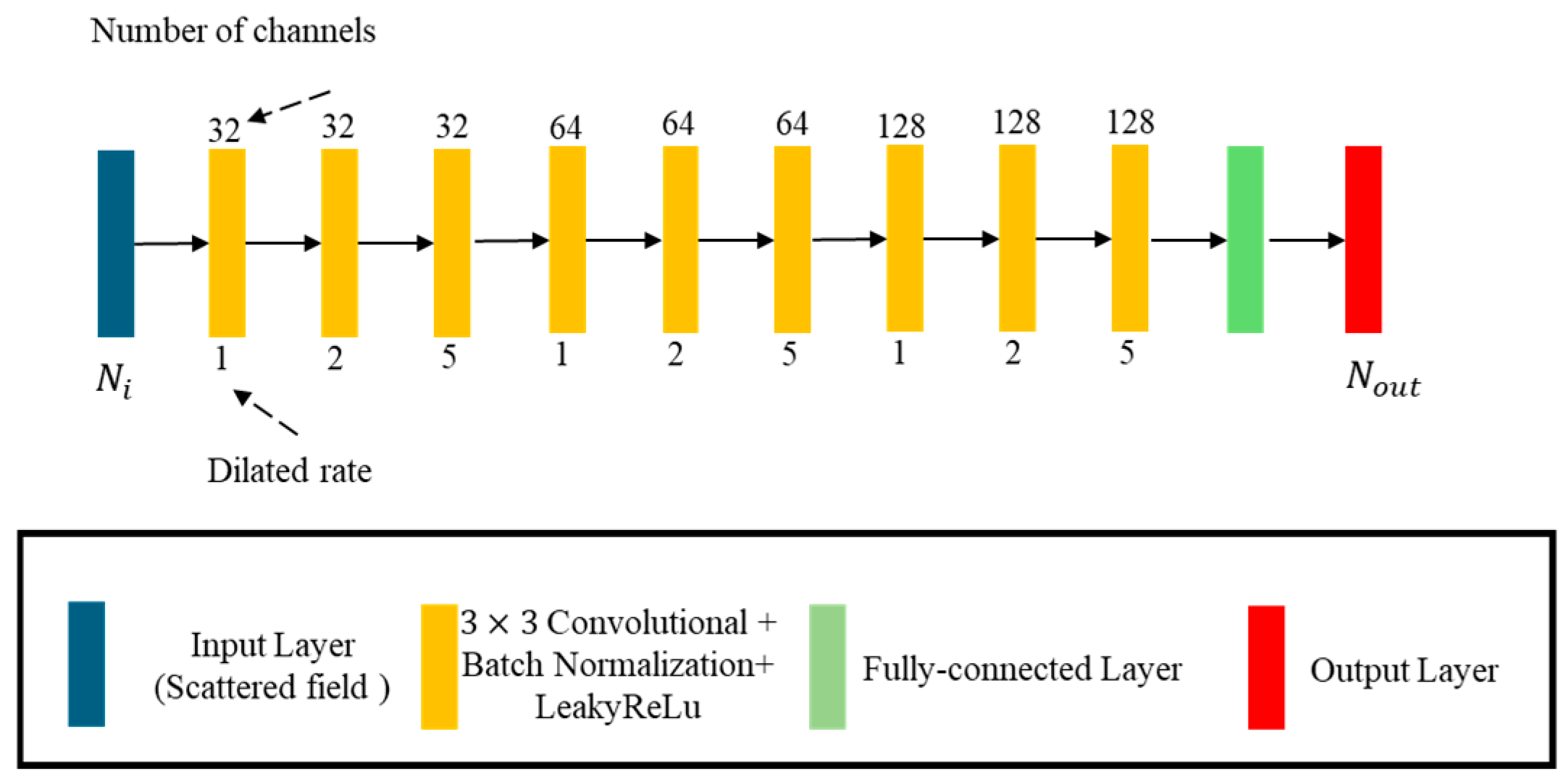
3. Deep Dilated Convolutional Neural Network

DDCNNs are sophisticated approaches within the domain of deep learning, as illustrated in Figure 2. These networks are designed to mimic the mathematical structure of the biological nervous system. They perform a hierarchy of operations across various levels and configurations to identify optimal and effective deep learning models. Unlike previous methods that require predefined human rules for machine learning, DDCNNs primarily need fine-tuning of trained models and hyperparameters within the designed neural architecture. This capability allows the system to autonomously discern features and compute optimal results. A key advancement in developing DDCNN is the continuous provision of high-quality datasets and rigorous computational training to improve model performance. The training process is often enhanced by utilizing advanced hardware, such as Graphics Processing Units (GPUs), along with optimized software frameworks. Training a DDCNN can be viewed as a “heterogeneous” process that involves transforming measured scattered fields into an initial shape within the object domain. The inputs to the DDCNN include the periodic, permittivity and shape components of the target. At the core of this architecture is the convolutional layer, which serves as a specialized neural layer for feature extraction from images. It accomplishes this by applying a smaller matrix, known as a convolutional kernel, over the image, generating compact feature vectors from localized regions. One of the key advantages of the convolutional layer is its ability to capture local patterns and textures, enabling the classification of objects regardless of their spatial positions within the image. The resulting feature vectors are then processed in a fully connected layer, which performs the final classification or regression task. This layer typically consists of multiple neurons, each connecting to feature vectors from the preceding convolutional and activation layers. Through these concatenations, the neural network effectively learns to associate the extracted features with the corresponding output classes or values, thereby facilitating accurate image reconstruction. This paper utilizes dilated convolution within the convolutional layers, a technique that enhances standard convolution by incorporating gaps or “holes” into the filter. This approach effectively augments the receptive field without imposing additional computational burdens, preserving the intrinsic benefits of conventional convolutions. As illustrated in Figure 3b, the receptive field resulting from three consecutive standard convolutions measures $7\times 7$. In contrast, the use of dilated convolutions of equivalent kernel size expands the receptive field dramatically to $17\times 17$. Differing from the linear relationship between the receptive field and layer depth observed in traditional convolutional networks (depicted in Figure 3a), the receptive field of dilated convolutions increases exponentially. Furthermore, dilated convolution has proven advantageous in streamlining the architecture of image reconstruction networks while concurrently decreasing computational costs [15]. We used the Adam optimizer to train the DDCNN. The training configuration includes a learning rate ranging from ${10}^{-3}$ to ${10}^{-4}$, and a maximum of 200 epochs.

In this paper, we input the measured scattered fields $E_s$ into the DDCNN module for training. A DDCNN expects the target to be the true periodic, permittivity and shape factor of the rough surface. Its loss function is expressed as follows:

$$los{s}_{DDCNN}={\displaystyle \frac{{‖Y-Y^i‖}_F}{{‖Y‖}_F}}$$

(17)

Let $Y$ denote the periodic length, permittivity and the true coefficients of the rough surface shape and $Y^i$ denote the reconstructed periodic length, permittivity and coefficients of the rough surface shape. The Frobenius norm is denoted by $F$.

4. Numerical Results

In our simulations, we explore 10,000 distinct rough surface profiles, partitioning the spatial domain into upper and lower halves. We split 80% of the data into a training database and the remaining data as a testing database. The upper half, designated as region 0, represents air, which is considered free space with a dielectric constant of $8.85\times {10}^{-12}$. While the lower half, labeled region 1, contains varying dielectric constants of 3.5, corresponding to varying periodic lengths of 0.04 m, 0.06 m, and 0.083 m, respectively. We illuminate a plane wave with a frequency of 3 GHz and a wavelength of 0.1 m at the periodic rough surface from region 0. To facilitate data collection, 32 incident plane waves are used to illuminate the rough surface and 32 receiving antennas that are evenly spaced at $y=1.5$ m are employed to record the scattered field from $x=-0.03875$ m to $x=0.03875$ m. To accurately simulate real-world conditions, Gaussian noise is introduced at levels of 5%, 10%, 15%, and 20%. The model encompasses eight unknown parameters, including the $N_f$ Fourier coefficients of the shape function, the periodic lengths, and the relative dielectric constants. For the Adam parameter configuration, we set the learning rate at ${10}^{-3}$ to ${10}^{-4}$. The mini-batch size is 32 and the maximum epoch is 200. Fourier expansion of the periodic rough surface is expressed as follows:

$$F\left(x\right)=\sum _1^{{\displaystyle \frac{N_f}{2}}}{a}_{n}cos(n·{\displaystyle \frac{2\pi x}{d}})+\sum _{{\displaystyle \frac{N_f}{2}}+1}^{N_f}{a}_{n}sin(n·{\displaystyle \frac{2\pi x}{d}})$$

(18)

where $N_f$ is set to 6 in the simulation. In order to obtain the performance of each scheme, we establish the following function:

$$DF={‖F^{pred}(x)-F^{exact}(x)‖}_F/{‖F^{pred}(x)‖}_F$$

(19)

$$DP={\displaystyle \frac{\left|d^{cal}-d^{exact}\right|}{d^{exact}}}$$

(20)

$$DEPS={\displaystyle \frac{\left|{\epsilon }^{cal}-{\epsilon }^{exact}\right|}{{\epsilon }^{exact}}}$$

(21)

DF and DP are used to calculate the deviation of the surface shape and the deviation of the period length d, respectively. On the other hand, DEPS is used to calculate the deviation of the relative dielectric constant ${\epsilon }_1$. $F^{exact}\left(x\right)$ and $F^{pred}\left(x\right)$ are the true and reconstructed rough surface profiles, respectively.

In practical scenarios, noise interference is prevalent and has a significant impact on reconstruction outcomes. Our analysis focuses on how various noise levels affect reconstruction quality, as illustrated in Figure 4, which shows the reconstruction of three irregular surface shapes under different noise levels. We also discuss the reconstruction results of different periods in this paper. Figure 4a–c explore the rough surfaces of the three wave peaks. Numerical results show that the first peak is characterized by its low height, and satisfactory reconstruction results can be obtained despite different noise levels. In contrast, the second and third peaks are higher and have steeper slopes, and the reconstruction quality decreases as the noise increases. Figure 4d–f explore the rough surfaces of the two wave crests. Numerical results show that satisfactory reconstruction results can be obtained for both peaks and troughs despite different noise levels. Figure 4g–i explore the rough surface of a wave crest. Numerical results show that the peak is affected by the period as well as the noise level. In other words, the slope of the peak is larger when the period is smaller, which affects the accuracy of reconstruction. On the contrary, as the period becomes longer, the slope of the peak becomes smaller, which improves the accuracy of the reconstruction. The DP, DPES and DF for the example are shown in

Table 1. Reconstruction performance of three rough surfaces with different periods.

	Period	0.04			0.06			0.083
Noise		DP	DEPS	DF	DP	DEPS	DF	DP	DEPS	DF
5%		0.09%	0.01%	10.45%	0.12%	0.1%	10.65%	0.1%	0.01%	7.32%
10%		0.1%	0.01%	10.94%	0.26%	0.13%	13.09%	0.1%	0.02%	7.90%
15%		0.12%	0.02%	12.06%	0.33%	0.19%	16.58%	0.13%	0.02%	9.45%
20%		0.14%	0.03%	15.93%	0.41%	0.26%	23.28%	0.15%	0.03%	10.34%

. It is clear that both DP and DEPS are less than 1%. Notably, our investigation indicates that under consistent shape parameters, a period of 0.083 results in a smoother surface shape and enhanced reconstruction quality due to its height and slope characteristics. Importantly, our method demonstrates a robust capability to accurately capture critical parameters such as periodicity, geometry, and relative permittivity, even on highly irregular surfaces in the presence of noise.

Furthermore, to demonstrate the effectiveness of our proposed method, we add the DCNN (without dilated convolution) for comparison. The numerical results show that the proposed method can obtain more accurate reconstruction results after adding the improvement of the dilated convolution machine.

Table 2. Comparison of reconstruction performance between DCNN and DDCNN over a period of 0.083.

	Period	DCNN			DDCNN
Noise		DP	DEPS	DF	DP	DEPS	DF
5%		0.18%	0.32%	13.9%	0.1%	0.01%	7.32%

presents the comparison of reconstruction performance between the DCNN and DDCNN.

Next, we test the trained model on a completely new dataset to verify the effectiveness of our proposed method. We input data with noise levels of 10%, 15%, and 20% into the 5% noise model to reconstruct the non-flat rough surface. Figure 5 shows that the proposed method has good noise immunity and can reconstruct the accurate shape of non-flat rough surfaces even in the presence of high noise. The DP, DEPS and DF for the experimental example are shown in

Table 3. Reconstruction performance for the new dataset.

	Period	0.083
Noise		DP	DEPS	DF
10%		0.1%	0.02%	8.80%
15%		0.15%	0.03%	10.45%
20%		0.21%	0.04%	11.34%

. The generalization ability of the model is evaluated by comparing Table 1 and Table 3. From Table 3, we can see that when using the new dataset, the reconstruction results are worse than those obtained with the test data, though they remain satisfactory. It is also observed that the performance of both DP and DF is below 1%.

In relation to the overall training duration for deep learning, the training time for the DDCNN model is 80 min using a personal computer equipped with a 3.8-GHz Intel Core i7 processor, 64 GB of RAM and NVIDIA RTX 4060 12 GB GPU. It is worth mentioning that once trained, our approach can quickly detect input data under 1 s.

5. Conclusions

This paper explores the application of electromagnetic imaging techniques to characterize periodic rough surfaces. We introduce a DDCNN architecture designed to concurrently reconstruct the surface shape, identify the periodicity, and determine the dielectric constant. Through our numerical simulations, we demonstrate the effective reconstruction of periodic lengths, relative permittivities, and surface geometries across various configurations. Our findings underscore the significant impact of artificial intelligence on the reconstruction of a non-flat rough surface. During the training process, we discover that the DDCNN prioritizes the accurate determination of surface periodicity, followed by the estimation of dielectric constants and then the shape. It is worth mentioning that our method uses dilated convolution to effectively enhance the receptive field without incurring an additional computational burden, retaining the inherent advantages of traditional convolution. This prioritization is influenced by the varying sensitivities of each coefficient to the scattered field data, reflecting the intricate relationship between these parameters during the reconstruction process. In the future, we plan to integrate more advanced neural networks, such as Generative Adversarial Networks (GANs), alongside attention mechanisms, to enhance the reconstruction accuracy for complicated rough surface profiles. By repeatedly generating more realistic rough surfaces through GANs, it helps to improve the accuracy of reconstruction. The limitation of our proposal is that when the surface shape is too steep, the dielectric constant is too large, and when the period is too small, the reconstruction performance is affected. In three-dimensional scenes, the high computing cost will be a major challenge.

References

1. El-Shenawee, M.; Miller, E.L. Multiple-Incidence and Multifrequency for Profile Reconstruction of Random Rough Surfaces Using the 3-D Electromagnetic Fast Multipole Model. IEEE Trans. Geosci. Remote Sens. 2004, 42, 2499–2510. [Google Scholar]
2. Firoozabadi, R.; Miller, E.L.; Rappaport, C.M.; Morgenthaler, A.W. Subsurface Sensing of Buried Objects Under a Randomly Rough Surface Using Scattered Electromagnetic Field Data. IEEE Trans. Geosci. Remote Sens. 2007, 45, 104–117. [Google Scholar]
3. Chen, Y.; Spivack, M. Rough Surface Reconstruction at Grazing Angles by an Iterated Marching Method. J. Opt. Soc. Am. A 2018, 35, 504–513. [Google Scholar]
4. Chiu, C.C.; Chan, M.K. Microwave Imaging of Periodic Rough Surfaces. Microw. Opt. Technol. Lett. 2018, 60, 1719–1727. [Google Scholar]
5. He, H.J.; Zhang, Y. An Effective Method for Electromagnetic Scattering from a Coated Object Partially Buried in a Dielectric Rough Surface. J. Electromagn. Waves Appl. 2020, 35, 754–765. [Google Scholar] [CrossRef]
6. Sefer, A.; Yapar, A. An Iterative Algorithm for Imaging of Rough Surfaces Separating Two Dielectric Media. IEEE Trans. Geosci. Remote Sens. 2021, 59, 1041–1051. [Google Scholar] [CrossRef]
7. Sefer, A.; Yapar, A. Image Recovery of Inaccessible Rough Surfaces Profiles Having Impedance Boundary Condition. IEEE Geosci. Remote Sens. Lett. 2022, 19, 3005105. [Google Scholar] [CrossRef]
8. Özdemir, Ö.; Altuncu, Y. A Microwave Subsurface Imaging Technique for Rough Surfaces. IEEE Geosci. Remote Sens. Lett. 2023, 20, 3003205. [Google Scholar]
9. Sefer, A.; Yapar, A.; Yelkenci, T. Imaging of Rough Surfaces by RTM Method. IEEE Trans. Geosci. Remote Sens. 2024, 62, 2003312. [Google Scholar]
10. Aydin, İ.; Budak, G.; Sefer, A.; Yapar, A. CNN-Based Deep Learning Architecture for Electromagnetic Imaging of Rough Surface Profiles. IEEE Trans. Antennas Propag. 2022, 70, 9752–9763. [Google Scholar] [CrossRef]
11. Aydin, İ.; Budak, G.; Sefer, A.; Yapar, A. Recovery of Impenetrable Rough Surface Profiles via CNN-Based Deep Learning Architecture. Int. J. Remote Sens. 2022, 43, 658–5685. [Google Scholar] [CrossRef]
12. Chiu, C.C.; Ho, C.S. Image Reconstruction of a Two-Dimensional Periodic Conductor by the Genetic Algorithm. J. Electromagn. Waves Appl. 2001, 15, 1175–1188. [Google Scholar] [CrossRef]
13. Bourlier, C.; Pinel, N.; Kubicke, G. Method of Moments for 2D Scattering Problems: Basic Concepts and Applications, 1st ed.; Wiley: New York, NY, USA, 2013. [Google Scholar]
14. Ishimaru, A. Electromagnetic Wave Propagation, Radiation, and Scattering; Prentice-Hall: Hoboken, NJ, USA, 1991. [Google Scholar]
15. Yu, F.; Koltun, V. Multi-Scale Context Aggregation by Dilated Convolutions. In Proceedings of the 4th International Conference on Learning Representations, San Juan, Puerto Rico, 2–4 May 2016. [Google Scholar]
Figure 1. Schematic diagram of the classic non-flat rough surface simulation.
Electronics 14 01236 g001
Figure 2. Deep dilated convolutional neural network architecture.
Electronics 14 01236 g002
Figure 3. Comparison of receptive fields between dilated and traditional convolutions. (a) Illustration of three 3 × 3 dilated convolutional layers with varying dilation rates r = 1 ,   2 ,   5 . (b) Illustration of three 3 × 3 traditional convolutional layers with a constant dilation rate of r = 0 .
Electronics 14 01236 g003
Figure 4. Reconstruction of the rough surfaces for different noise levels and periodic lengths: (a) periodic length of 0.04 m for the first example; (b) periodic length of 0.06 m for the first example; (c) periodic length of 0.083 m for the first example; (d) periodic length of 0.04 m for the second example; (e) periodic length of 0.06 m for the second example; (f) periodic length of 0.083 m for the second example; (g) periodic length of 0.04 m for the third example; (h) periodic length of 0.06 m for the third example; (i) periodic length of 0.083 m for the third example.
Electronics 14 01236 g004
Figure 5. Reconstruction of the surfaces for the new dataset.
Electronics 14 01236 g005