Research on Lightweight Facial Landmark Prediction Network

Abstract

Facial landmarks, as direct and reliable biometric features, are widely utilized in various fields, including information security, public safety, virtual reality, and augmented reality. Facial landmarks, which are discrete key points on the face, preserve expression features and maintain the topological structure between facial organs. Fast and accurate facial landmark prediction is essential in solving computer vision problems involving facial analysis, particularly in occlusion scenarios. This research proposes a lightweight facial landmark prediction network for occluded faces using an improved depthwise separable convolutional neural network architecture. The model is trained using 30,000 images from the CelebA-HQ dataset. The model is then tested under different occlusion ratios, including 10–20%, 30–40%, 40–50%, and 50–60% random occlusion, as well as 25% center occlusion. Using 68 facial landmarks for occlusion prediction, the proposed method always achieved significant improvements. Experimental results show that the proposed lightweight facial landmark prediction method is 1.97 times faster than FAN* and 1.67 times faster than ESR*, while still achieving better prediction results with lower NMSE values across all tested occlusion ratios for both frontal and profile faces.

1. Introduction

With the rapid development of artificial intelligence and computer vision research, human society has gradually shifted from the industrialization and informatization stage to the intelligence stage. The computer vision problem based on biometric features not only has academic value but also has enormous application prospects and market value in the industrial sector. The human face is one of the most important organs that humans possess. The appearance, posture, and expressions of the face contain rich information and are potentially strongly related to a person’s identity, emotions, and actions. Computer vision problems based on facial features have naturally become a research hotspot. Facial landmark prediction is a prerequisite for related computer vision problems based on facial features. The purpose of facial landmark prediction is to locate the key points of facial organs, such as eye frames, eyebrows, nose, etc. The prediction results can be applied to various tasks, including facial recognition [1], head pose estimation [2], facial reconstruction [3], and three-dimensional facial reconstruction [4], among others.

The research on facial landmark prediction mainly focuses on learning distinguishable features from a large number of deformations in facial shape and posture, different expressions, partial occlusion, and other situations [5]. A very typical methodological framework is to construct features through convolutional neural networks or manually constructed features to describe the appearance and shape information of a face and then apply a model, namely, a regression model, to map the features to the positions of landmarks [6,7]. They mostly adopt a cascade strategy to concatenate prediction modules and gradually update the predicted positions of landmarks [8]. However, the performance of the cascaded regression method deteriorates when initialization is inaccurate, and when there are a large number of self-focusing landmarks or large in-plane rotations, facial poses become larger. Based on this situation, Bulat and Tzimiropoulos proposed a fully convolutional network based on heatmap regression [9]. This facial landmark detection technique has better detection accuracy and is more suitable for practical applications.

In deep learning based facial landmark prediction, occlusion is an important challenge. Occlusion may result in a decrease in the performance of landmark prediction algorithms due to the partial occlusion of key facial features by objects such as hair, hands, glasses, and masks. Shao et al. proposed a reinforcement learning framework that enables the model to learn how to select the most reliable keypoints in occluded situations, thereby improving the accuracy of localization [10]. Xiong and De la Torre proposed the supervised descent method (SDM), which iteratively optimizes the position of keypoints and combines local region features [6]. SDM can effectively locate facial landmarks in occluded situations, but iterative optimization may result in slow testing speed. How to quickly and accurately predict facial landmarks under occlusion is the problem that needs to be addressed in the research. In 2017, Google’s research team proposed the MobileNet. MobileNet is a lightweight deep learning neural network designed to significantly reduce model size and accelerate model computation speed without sacrificing model performance. Researchers have developed MobileNetV1, MobileNetV2, and MobileNetV3 network models through model iteration [11]. A lightweight deep learning network based on MobileNet is proposed to improve the lightweight facial landmark prediction network.

2. MobileNetV3 Architecture

Compared to regular convolutional neural networks, MobileNetV3 adopts a deep convolutional neural network architecture and introduces the inverted residuals structure, making the layer structure more efficient. It incorporates a lightweight attention module based on the squeeze-and-excitation network (SENet) in the bottleneck structure, uses the h-swish activation function, and employs 1 × 1 convolutions to build the final layer of the network. This approach increases the dimensionality of the feature matrix, making the features more abundant.

The depthwise separable convolution operation can be decomposed into two steps: depthwise convolution and pointwise convolution, as shown in Figure 1. Depthwise convolution, also known as channel-wise convolution, applies a convolution kernel independently to each input channel. Each input channel is processed using only one convolution kernel, generating one output channel. The number of resulting feature maps matches the number of input channels. For example, if a 5 × 5 pixel, three-channel image is used as input, and it is processed with three 3 × 3 convolution kernels in a depthwise convolution, the final output will be a three-channel feature map. Pointwise convolution can be seen as a special case of standard convolution, where the convolution kernel size is 1 × 1. The output features from depthwise convolution are linearly combined across channels to generate new features, with the number of resulting features equal to the number of convolution kernels used.

Assuming $M$ is the number of channels in the input layer, $N$ is the number of channels in the output layer, $D_F$ is the spatial width and height of the input feature map, and $D_K$ is the spatial size of the convolution kernel [12], the standard convolution layer takes the feature map of $D_F\times D_F\times M$ as input and the convolution kernel parameters are $D_K\times D_K\times M\times N$. Assuming that the generated feature map has the same size as the input, it generates a feature map of $D_F\times D_F\times N$, where $D_F$ is the spatial width and height of the input feature map, $D_K$ is the spatial size of the convolution kernel, $M$ is the number of input channels (input depth), and $N$ is the number of output channels (output depth). The computational cost depends on the product of the number of input channels $M$, the number of output channels $N$, the size of the convolution kernel $D_K\times D_K$, and the size of the input feature map $D_F\times D_F$. The computational cost of standard convolution is obtained as $D_K\cdot D_K\cdot M\cdot N\cdot D_F\cdot D_F$.

Depthwise separable convolution consists of two layers: deep convolution and point convolution. We use deep convolution to apply a single filter on each input channel (input depth). Then, we use pointwise convolution (a simple 1 × 1 convolution) to create a linear combination of deep layer outputs. MobileNetV1 uses batch normalization (BN) and rectified linear unit (ReLU) nonlinear excitation functions for both layers. The convolution kernel parameters for deep convolution are $D_K\times D_K\times 1\times M$, and the computational cost of deep convolution is $D_K\cdot D_K\cdot M\cdot D_F\cdot D_F$.

Deep convolution is very effective compared to standard convolution. However, it only filters the input channels and does not combine them to generate new features. Therefore, a 1 × 1 point convolutional layer is needed to calculate the linear combination of deep convolution outputs in order to generate these new features. The convolution kernel parameters of point convolution are $1\times 1\times M\times N$, and the computational cost of point convolution is $M\cdot N\cdot D_F\cdot D_F$.

In summary, the computational cost of depthwise separable convolution is $D_K\cdot D_K\cdot M\cdot D_F\cdot D_F+M\cdot N\cdot D_F\cdot D_F$.

By decomposing depthwise separable convolutions, the computational cost is reduced to the following:

$${\displaystyle \frac{D_K\cdot D_K\cdot M\cdot D_F\cdot D_F+M\cdot N\cdot D_F\cdot D_F}{D_K\cdot D_K\cdot M\cdot N\cdot D_F\cdot D_F}}={\displaystyle \frac{1}{N}}+{\displaystyle \frac{1}{D_K^2}}.$$

(1)

When MobileNet uses a 3 × 3 convolution kernel for depthwise separable convolution, the computational cost is eight to nine times less than that of the standard convolution.

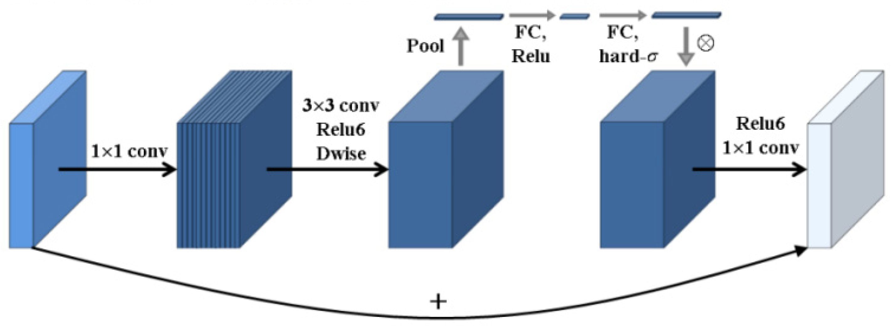
The inverted residuals structure is introduced, and the nonlinear activation function after convolution is replaced with a linear activation function, making the layer structure more efficient. A lightweight attention module based on SENet is incorporated into its bottleneck structure. The specific architecture is shown in Figure 2 [13,14,15]. The SENet attention module is placed after the depthwise convolution in the expansion module, with the aim of maximizing the expressive power of the attention module and enhancing feature extraction capabilities.

The inverted residuals structure model is quite similar to the reverse operation of the traditional residual block. First, a 1 × 1 convolution operation is performed to expand the feature map dimensions. Then, a 3 × 3 depthwise convolution is applied for filtering, followed by a 1 × 1 pointwise convolution to further increase the feature map dimensions. The resulting model has a spindle shape, with a larger middle and smaller ends. A new activation function, ReLU6, is used, which is robust when combined with low-precision computation. The inverted residual block first increases the dimension and then reduces it, extracting more features compared to the traditional residual block.

The MobileNetV3 network uses 1 × 1 convolution to construct the final layer of the network in order to increase the dimension of the feature matrix and make the features more abundant, but this will increase the computational complexity. Therefore, performing mean pooling on the features after 1 × 1 convolution not only preserves the high-dimensional information of the image but also reduces computational complexity and latency. The schematic diagram of the final stage of network modification is shown in Figure 3.

The hard swish (h − swish) activation function [16] used is represented as follows:

$$\mathrm{h}-\mathrm{swish}\left[x\right]=x{\displaystyle \frac{ReLU6\left(x+3\right)}{6}}$$

(2)

where $x$ is the output of the corresponding layer in the network. MobileNetV3 can be divided into the MobileNetV3-large model, which is suitable for high-resource environments, and the MobileNetV3-small model, which is designed for low-resource environments. The overall structure of both large and small models is the same, with the key differences being the number of basic units (Bneck) and internal parameters, primarily the number of channels. This research aims to design a lightweight network with low computational cost and faster testing speed; thus, improvements are made based on the MobileNetV3-small model [17].

3. Improved Lightweight Facial Landmark Prediction Network

Facial landmarks can be regarded as discrete points sampled from key regions of the face. The structure formed by these discrete points retains the facial expression features and preserves the topological relationships between different facial organs. This study improves upon the MobileNetV3-small network by introducing SENet. To address the issue that SENet’s training of keypoints is difficult to converge, the network is further enhanced using depthwise separable convolution, batch normalization, inverted residual structure, linear bottleneck structure, and average pooling. The landmark prediction module is trained using the landmark prediction loss $L_{\mathrm{lmk}}$, resulting in the construction of a lightweight facial landmark prediction network for 256 × 256 sized facial images.

3.1. Construction of Landmark Prediction Network

For facial restoration networks, the issue to address is the underlying topology and attributes, not just the precise location of individual landmarks. Therefore, establishing a facial image topology landmark prediction network will effectively enhance the image restoration performance. The input to the facial landmark prediction network is obtained by performing the Hadamard product of the facial image and the generated mask to produce the occluded image. Let $I^M$ be the occluded facial image, $I$ be the facial image, and $M$ be the mask. The occluded image $I^M$ is represented by the following formula.

$$I^M:=I\circ M$$

(3)

Assuming $M_L$ is a feature point prediction network, ${\theta }_L$ is the training parameter of the network, and $\widehat{L}$ is the predicted feature point, then

$$\widehat{L}\in R^{2\times n}:=M_L\left(I^M;{\theta }_L\right).$$

(4)

The function of the landmark prediction network $M_L$ is to obtain 68 facial landmarks from the occluded facial image $I^M$.

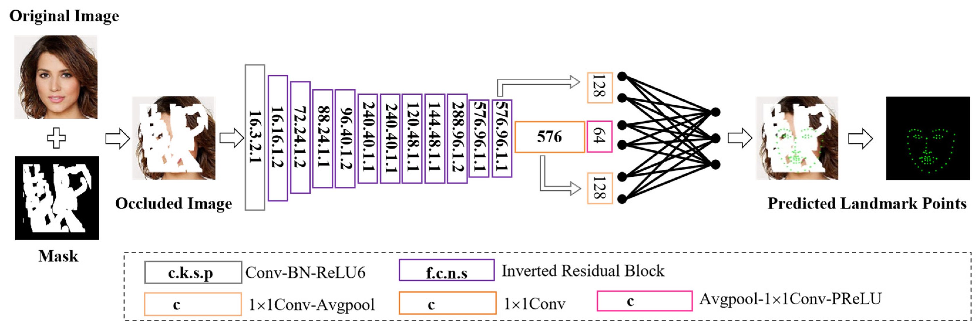
The facial landmark prediction network uses depthwise separable convolution, inverted residual structure, linear bottleneck structure, average pooling(Avg-Pool), etc., to address the problem of their being difficulty in converging keypoint training with SENet. The network structure is shown in Figure 4.

The first 13 convolutional layers use 11 bottleneck (bneck) structures to extract features and accelerate the network speed. The next 10 convolutional layers compress the extracted feature maps. The final layer of the network is a fully connected layer that merges the processed feature maps and maps them to the sample image, thereby outputting the facial landmarks of the occluded image. The specific structure of the improved facial landmark prediction network is shown in Figure 5. In the figure, c represents the output channel number, k is the kernel size, s is the convolution or deconvolution stride, p is padding, f is the dilation factor, and n is the number of repetitions.

Table 1. Network structure parameters of the improved landmark prediction module.

Input	Operator	Exp Size	c	SE	NL	s
2562 × 3	conv2d, 3 × 3	-	16		HS	2
1282 × 16	bneck, 3 × 3	16	16	√	RE	2
642 × 16	bneck, 3 × 3	72	24		RE	2
322 × 24	bneck, 3 × 3	88	24		RE	1
322 × 24	bneck, 5 × 5	96	40	√	HS	2
162 × 40	bneck, 5 × 5	240	40	√	HS	1
162 × 40	bneck, 5 × 5	240	40	√	HS	1
162 × 40	bneck, 5 × 5	120	48	√	HS	1
162 × 48	bneck, 5 × 5	144	48	√	HS	1
162 × 48	bneck, 5 × 5	288	96	√	HS	2
82 × 96	bneck, 5 × 5	576	96	√	HS	1
82 × 96	bneck, 5 × 5	576	96	√	HS	1
82 × 96 (C1)	conv2d, 1 × 1	-	576	√	HS	1
82 × 576 (C2)	pool, 8 × 8	-	-	-	-	1
12 × 576	conv2d 1 × 1, NBN	-	1024	-	HS	1
1 × 1 × 1024	conv2d 1 × 1, NBN	-	64	-	-	1
1 × 1 × 64 (S3)	-	-	64	-	-	-
C1	conv2d 1 × 1	-	128	-	-	1
82 × 128	Avg-Pool 8 × 8	-	128	-	-	-
1 × 1 × 128 (S1)	-	-	128	-	-	-
C2	conv2d 1 × 1	-	128	-	-	1
82 × 128	Avg-Pool 8 × 8	-	128	-	-	-
1 × 1 × 128 (S2)	-	-	128	-	-	-
S1, S2, S3	Full Connection	-	136	-	-	-

shows the structural parameters of the improved landmark prediction network. In the table, SE represents whether there is an SE module, NL represents the type of nonlinear impulse function used, HS represents the h-swift impulse function, RE represents the ReLU impulse function, NBN represents no batch normalization, Conv2d represents two-dimensional convolutional layer, Avg-Pool represents average pooling, SE represents squeeze-and-excitation network, c represents the output channel number, and s represents the step size. The input image selected by this network is a 256 × 256 three channel image. Each row in the table represents a convolutional layer.

3.2. Loss Function

The landmark prediction loss $L_{\mathrm{lmk}}$ is used to train the landmark prediction module ${{\rm M}}_L$, which measures the fit between the generated landmark $\widehat{L}$ and the real landmark $L_{\mathrm{gt}}$. The training loss is as follows.

$$L_{\mathrm{lmk}}\hspace{0.33em}:={\Vert \widehat{L}-L_{\mathrm{gt}}\Vert }_2^2$$

(5)

This loss is used to generate landmarks for facial image contours, ensuring the topological structure between facial organs [18].

3.3. Training Environment

The training and testing in the study were conducted on a server equipped with the Windows 10 Professional operating system. The main parameters of the server are as follows: hardware configuration includes a CPU (Inter Xeon, Intel Corporation, Santa Clara, CA, USA) and four GPUs (Nvidia TITAN Xp, NVIDIA Corporation, Santa Clara, CA, USA); memory is Micron 256 GB; and hard disk is 2 TB. All experiments in this article are based on PyTorch 1.10.0’s deep learning framework. PyTorch is an optimized tensor library that uses GPU and CPU for deep learning. Formerly known as Torch, it is a deep learning framework primarily based on Python. It is not only fast and efficient but also supports dynamic neural networks while achieving powerful GPU acceleration. Compared to the TensorFlow framework, its framework is more concise.

3.4. Training Parameters and Data Processing

The experiment uses a subset of 30,000 images with a resolution of 256 × 256 from the CelebA-HQ dataset for training the landmark prediction network [19]. The downloaded CelebA-HQ dataset is divided into three parts: 29,500 images for the training set, 200 images for the validation set, and 300 images for the test set.

During the training process, the Adma optimizer with exponential decay rates of $\beta 1=0$ and $\beta 2=0.9$ was used for optimization [20,21]. The Adam optimizer combines the advantages of a momentum method and adaptive learning rate to provide an efficient, stable, and easy-to-use optimization solution that converges faster than traditional SGD or Momentum. The parameter settings during training are as follows: set the learning rate to 0.0001, the batch size for image processing to 16, and the number of iterations to wait before saving the model to 1000. The number of iterations to wait between samples is set to 1000, the number of images to be sampled each time is set to 4, the number of iterations to wait during the model evaluation process is set to 0, and the number of iterations to wait for recording the training status is set to 100.

4. Prediction Results and Discussion

4.1. Facial Landmark Prediction Under Mask Occlusion

In order to test the performance of the proposed improved lightweight facial landmark prediction model on occluded face images, the test images are generated by combining the original images with masked images. The original images are from the test set reserved in the CelebA-HQ dataset, and the masked images are from the test portion of the mask dataset provided by Liu et al. The mask dataset is divided into six categories based on different coverage area ratios, with coverage ratios ranging from 0–10%, 10–20%, 20–30%, 30–40%, 40–50%, and 50–60%. In order to consider various situations of facial occlusion and severe occlusion in the testing experiment, we chose random mask images with coverage ratios of 10–20%, 30–40%, 40–50%, and 50–60% in the mask dataset, as well as a central mask with a coverage ratio of 25%, for the landmark prediction experiment of the training model.

Figure 6 shows the 68 facial key points annotated by the prediction network. Among these, there are 10 key points for the eyebrows, with 5 points uniformly sampled from the left to the right boundary of each eyebrow. The eyes have 12 key points in total, with each eye having 6 points uniformly sampled from the left and right boundaries and the upper and lower eyelids. The lips comprise 20 key points, with 2 points at each corner of the mouth, 5 points uniformly sampled along the outer boundary of the upper and lower lips, and 3 points along the inner boundary. The nose has 9 key points, with 4 points along the bridge of the nose and 5 points uniformly sampled at the tip of the nose. The facial contour is represented by 17 uniformly sampled key points.

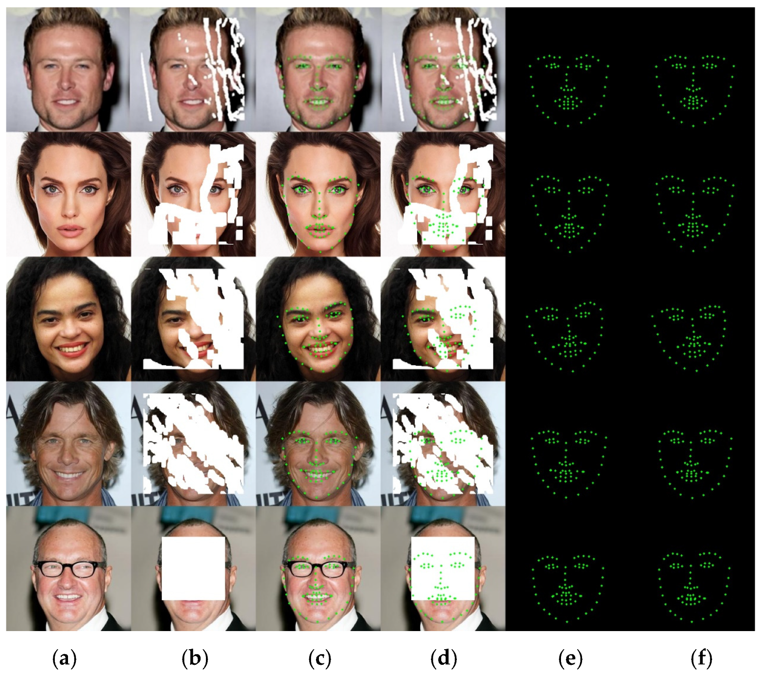
Figure 7 shows the experimental comparison of the model’s prediction of facial landmarks on the original image of a frontal face and four types of mask occlusions. The first row of the mask in the image accounts for 10–20% of the image, the second row accounts for 30–40%, the third row accounts for 40–50%, the fourth row accounts for 50–60%, and the fifth row is the central mask that accounts for 25%. The landmarks predicted by this model are the positions of key facial parts (eyebrows, eyes, nose, lips, facial contours), so when non-predicted facial areas (such as face and forehead) are obscured, it does not affect the prediction effect. As shown in the first, second, and third rows of the figure, when the occlusion area of the key part is small, the predicted landmark positions are basically consistent with the real landmark positions. The difference is that the first row predicts the right eye, the second row predicts the mouth, and the third row predicts the eyebrow landmark positions with some changes. As the occlusion area of key parts increases, the predicted positions of various organ landmarks change to some extent compared to the original image, such as the eyebrows, lips, and facial contours predicted in the fourth row, and the eyebrows, lips, and nose predicted in the fifth row. From the prediction results of different occlusion situations, it can be seen that although the predicted landmarks of each organ have certain deviations from the original image, the overall structure maintains the topological structure between facial organs, and the predicted landmarks basically restore the facial expression information of the original image.

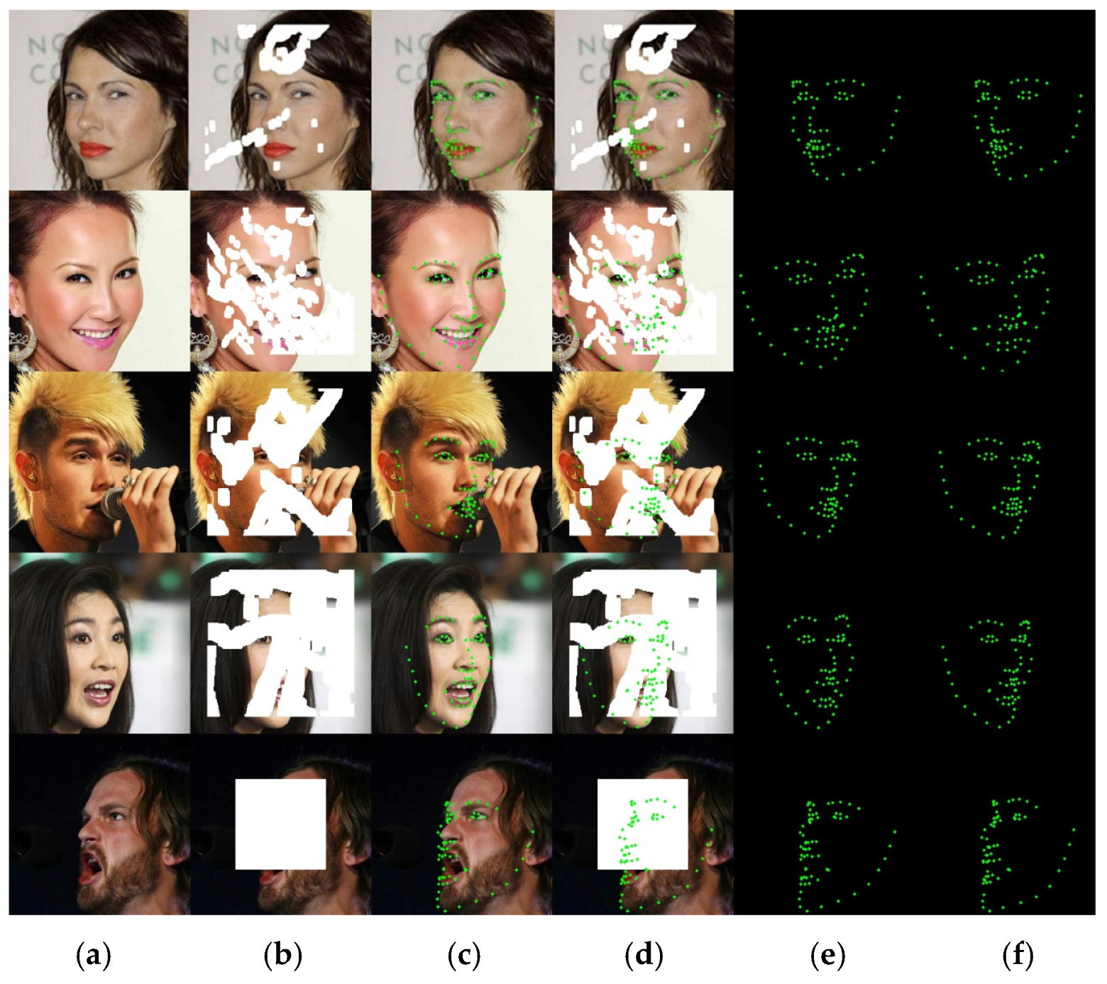
Figure 8 shows a comparison of the model’s predictions of facial landmarks between the original image of the side face and the facial landmarks after four mask occlusions. The first row of the mask in the image accounts for 10–20% of the image, the second row accounts for 30–40%, the third row accounts for 40–50%, the fourth row accounts for 50–60%, and the fifth row is the central mask that accounts for 25%. In the first and second rows of the figure, when the occlusion area of the key part is small, the predicted landmark positions are basically consistent with the real landmark positions. The difference is that the nose predicted in the first row and the mouth landmark positions predicted in the second and third rows have changed. The occlusion areas in the fourth and fifth rows are relatively large, and the predicted positions of various organ landmarks have some changes compared to the original image, such as the right eyebrow, nose, and facial contours predicted in the fourth row, and the eyebrows, nose, and lips predicted in the fifth row. The results show that the model also has excellent predictive ability for lateral faces. Except for small deviations in some organ landmarks, the overall prediction results also maintain the topological structure and facial expression information between facial organs.

From the prediction results of different occlusion situations on the front and side faces, it can be seen that although the predicted landmarks of each organ have certain deviations from the original image, the larger the occlusion area, the greater the deviation of the predicted 68 landmarks. However, the overall structure of the facial organs is maintained, and the predicted landmarks basically restore the facial expression information of the original image.

4.2. Experimental Results and Indicator Testing

Measure the computational speed of the model through testing time. In addition, considering the influence of irrelevant factors such as image size and facial angle on the evaluation, the normalized mean square loss function of pupil distance was used to test and analyze the experimental results. The normalized mean square loss function is as follows.

$$\mathrm{NMSE}={\displaystyle \frac{{{\displaystyle \sum }}_{i=1}^N{\Vert x_{\left(i\right)}^e-x_{\left(i\right)}^g\Vert }_2}{N\times d_{ipd}}}$$

(6)

In the formula, $d_{ipd}$ represents the distance between the pupils of the face’s eyes, which is used to normalize the face and eliminate the influence of different face sizes; $x_{\left(i\right)}^e$ represents the predicted position of the landmark corresponding to the i-th face; and $x_{\left(i\right)}^g$ represents the true position of the landmark corresponding to the i-th face. The average of the errors obtained from all faces is the final result.

To validate the effectiveness of the facial landmark prediction network in this study, the results from the MobileNet-L network were compared with those from the FAN and ESR networks. FAN is a deep learning model specifically designed for high-precision facial keypoint detection. It can handle occlusion issues to some extent but relies on the diversity of training data and the model’s generalization ability. ESR is a regression-based model proposed by Cao Xudong in “Face Alignment by Explicit Shape Regression” at CVPR 2012, which has achieved impressive results. For the purpose of accurate comparison, this study reproduced FAN and ESR, represented by FAN* and ESR*, respectively.

Table 2. Testing speed using different methods.

Method	FAN*	ESR*	MobileNet-L
Times (s)	3.64	3.06	1.84

displays the testing times for facial feature localization using FAN*, ESR*, and the MobileNet-L network.

From Table 2, it can be seen that MobileNet-L using deep convolution has a testing speed that is nearly 1.97 times faster than FAN* and nearly 1.67 times faster than ESR*, indicating a significant improvement in testing speed.

Table 3. NMSE under different coverage ratios of frontal faces.

Method	10–20%	30–40%	40–50%	50–60%	25% Center Occlusion
FAN*	3.56	4.75	6.85	7.82	9.52
ESR*	4.72	6.53	9.63	10.34	13.26
MobileNet-L	2.64	3.67	5.75	6.26	9.54

shows the NMSE of different algorithms under different coverage ratios of frontal faces.

From Table 3, it can be seen that when the frontal face is slightly occluded (10–20% coverage), each model performs well, with relatively low NMSE, indicating that the model can accurately locate landmarks in small-area occlusion situations.

When there is moderate occlusion (30–40% coverage), severe occlusion (40–50% coverage), and severe occlusion (50–60% coverage), the positioning errors of each model gradually increase with the increase in coverage. When the center occupies 25% of the cover, the positioning error significantly increases due to most of the face being obscured. When the coverage rate is between 10% and 60%, the MobileNet-L model outperforms the FAN* and ESR* models. When the center coverage rate is 25%, the positioning error of the ESR* model significantly increases, while the errors of the MobileNet-L and FAN* models are close.

Table 4. NMSE under different coverage ratios of side faces.

Method	10–20%	30–40%	40–50%	50–60%	25% Center Occlusion
FAN*	4.02	6.78	11.06	12.67	14.07
ESR*	4.75	6.73	10.93	12.42	13.86
MobileNet-L	5.36	7.25	10.27	11.8	12.13

shows the NMSE of different algorithms under different coverage ratios of the side face.

Comparing Table 3 and Table 4, it can be seen that the NMSE of each model is significantly higher for the side face compared to the corresponding data for the front face. The higher the coverage ratio of occlusion, the greater the positioning error. In mild and moderate occlusion, the MobileNet-L model has a slightly larger localization error than the FAN* and ESR* models. In severe occlusion and occlusion with a center-to-center ratio of 25%, the MobileNet-L model outperforms the FAN* and ESR* models.

Figure 9 shows the experimental results of the network framework ablation study. When the center is occluded, the introduction of SE in the network framework improves the prediction performance by 3.5%. When using h-swift, the prediction performance improves by 11.6%. When using a linear bottleneck structure, the prediction performance improves by 9.2%. When introducing an inverted residual structure, the prediction performance improves by 17.8%. The experimental results indicate that the improvement of network structure is effective.

5. Conclusions

This study constructs a lightweight facial landmark prediction network, incorporating SENet. To address the issue of SENet’s difficulty in converging during landmark training, improvements such as depthwise separable convolutions, reverse residual structures, linear bottleneck structures, and average pooling are adopted. The landmark prediction module is trained using the landmark prediction loss $L_{\mathrm{lmk}}$. Through model training, facial landmark prediction is achieved under different occlusion conditions. The experimental results show that this network can accurately predict facial landmarks under mask occlusion, and the predicted landmarks maintain the topological structure and expression information of the face. At the same time, the testing speed is nearly 1.97 times faster than FAN* and nearly 1.67 times faster than ESR*, indicating a significant improvement in testing speed.