An Efficient Convolutional Neural Network Accelerator Design on FPGA Using the Layer-to-Layer Unified Input Winograd Architecture

Abstract

Convolutional Neural Networks (CNNs) have found widespread applications in artificial intelligence fields such as computer vision and edge computing. However, as input data dimensionality and convolutional model depth continue to increase, deploying CNNs on edge and embedded devices faces significant challenges, including high computational demands, excessive hardware resource consumption, and prolonged computation times. In contrast, the Decomposable Winograd Method (DWM), which decomposes large-size or large-stride kernels into smaller kernels, provides a more efficient solution for inference acceleration in resource-constrained environments. This work proposes an approach employing the layer-to-layer unified input transformation based on the Decomposable Winograd Method. This reduces computational complexity in the feature transformation unit through system-level parallel pipelining and operation reuse. Additionally, we introduce a reconfigurable, column-indexed Winograd computation unit design to minimize hardware resource consumption. We also design flexible data access patterns to support efficient computation. Finally, we propose a preprocessing shift network system that enables low-latency data access and dynamic selection of the Winograd computation unit. Experimental evaluations on VGG-16 and ResNet-18 networks demonstrate that our accelerator, deployed on the Xilinx XC7Z045 platform, achieves an average throughput of 683.26 GOPS. Compared to existing approaches, the design improves DSP efficiency (GOPS/DSPs) by 5.8×.

1. Introduction

Convolutional Neural Networks (CNNs) have recently become central to fields such as artificial intelligence and edge computing, with applications spanning image recognition [1], autonomous driving [2], and natural language processing [3]. However, the increasing dimensionality of input data and the depth of convolutional models have placed greater demands on the performance of fundamental operations such as matrix multiplication (MM) [4,5]. This surge in computational complexity and power consumption limits the feasibility of deploying CNNs on edge devices. Moreover, growing concerns about user data privacy are expected to accelerate the adoption of model training on edge devices [6]. Consequently, there is an urgent need to develop efficient training and inference techniques for edge devices.

Currently, central processing units (CPUs), constrained by throughput limitations and serial execution, fail to meet the real-time processing requirements of delay-sensitive CNN applications. Graphics processing units (GPUs), designed for high bandwidth and computational parallelism, are optimized for matrix operations, making them well suited for real-time CNN processing [7]. For example, the NVIDIA A100 has demonstrated a performance capability of 19.5 TFLOPS. However, due to their high power consumption, GPUs are typically deployed in data centers, as they cannot satisfy the low power requirements of edge devices. In contrast, field-programmable gate arrays (FPGAs), with their high parallelism and reconfigurability, offer a promising solution for CNN acceleration, providing advantages in both flexibility and energy efficiency [8,9]. Thus, achieving high throughput performance (GOPS) and power efficiency (GOPS/W) in edge system designs is crucial for the practical deployment of CNNs [10]. A major challenge in this area is balancing the trade-off among network accuracy, computational performance, and power consumption [11]. Given that convolutional operations account for over 90% of the computational workload in CNNs [12], reducing their complexity through algorithmic optimizations is key to improving computational efficiency. To address these challenges and enhance the speed and inference capabilities of CNNs, researchers have proposed several algorithms.

2. State of the Art in CNN Acceleration Algorithms

The current mainstream convolution acceleration algorithms include GEMM (General Matrix Multiplication), FFT (Fast Fourier Transform), and the Winograd algorithm. The FFT algorithm transforms convolutions into the frequency domain, thereby reducing the number of multiplication operations. However, since its performance is positively correlated with the size of the convolution kernel [13], the FFT algorithm offers limited performance improvements for mainstream CNN models [14]. The Winograd convolution algorithm applies the Winograd method to two-dimensional convolution in neural networks. It reduces the computational complexity of small convolutions by transforming convolution operations into a series of minimal filtering operations, significantly reducing the number of multiplications required. Nevertheless, it is only applicable to convolutions with a stride of one [15]. A hybrid algorithm combining Winograd and GEMM was proposed, but it resulted in substantial resource consumption [16]. Furthermore, by utilizing a fused data path to support both conventional and Winograd convolutions within the same architecture, good energy efficiency was achieved. However, most of these accelerators are constrained by throughput performance.

To enhance accelerator throughput performance, a multi-PE (Processing Element) accelerator architecture based on a row-level pipeline strategy was proposed, effectively increasing throughput [17]. However, this approach leads to excessive consumption of computational resources and inefficient utilization of DSPs (Digital Signal Processors). To achieve better DSP utilization in CNN accelerators, studies [18,19] have explored various methods. They proposed hardware block convolution designs and software–hardware collaborative designs, respectively, effectively optimizing DSP utilization. Nonetheless, their fixed hardware compute unit designs lack the capability to handle kernels of varying sizes and strides, thereby restricting their application scope. Furthermore, to address computational resource utilization issues, a unified hardware architecture with adaptive allocation of Winograd units was proposed, significantly improving throughput [20]. However, this results in a substantial increase in power consumption, making it unsuitable for edge device applications.

Regarding the power efficiency of CNN accelerators, a Tensor Processing Unit (TPU) was introduced, achieving significant improvements in energy efficiency [21]. However, this enhancement comes at the expense of accelerator performance, limiting its applicability to specific scenarios.

To enhance the performance of CNN accelerators, previous studies have employed various optimization methods and hardware designs. Nevertheless, most of these approaches have failed to achieve an optimal balance between computational performance and power consumption. Additionally, unified computational architectures necessitate the use of Winograd computing units with fixed kernel sizes and strides. This requirement leads to computational challenges when convolution layer parameters change, resulting in mismatches between convolution sizes and the Winograd computing units.

To address the limitations of the Winograd method, kernel decomposition-based schemes have been introduced in several works. For instance, Ref. [22] proposed a convolution decomposition method that adapts the Winograd algorithm to different types of convolutions while reducing on-chip resource utilization. Building on the Winograd algorithm, Ref. [23] improved support for convolutions and transposed convolutions with strides greater than one. Additionally, Ref. [24] introduced a Winograd algorithm for large-scale decompositions and non-unit stride convolutions, helping reduce computational complexity without sacrificing precision. These kernel decomposition-based methods allow for flexible computations across various types of convolutions.

However, these direct kernel decomposition approaches are constrained by variations in convolution input block sizes, kernel sizes, and stride lengths. Moreover, they have not achieved an ideal balance between overall accelerator performance and power consumption. To overcome these challenges, we propose a layer-to-layer unified input-blocking decomposable Winograd method. This approach enables dynamic matching between convolution layer parameters and computing units, facilitating corresponding acceleration on a per-layer basis. The main contributions of this paper are summarized as follows:

• To address the issues associated with existing direct kernel decomposition methods and varying convolution parameters, we introduce a reconfigurable Winograd method featuring layer-to-layer unified input-blocking. This method mitigates performance limitations arising from decomposing kernels of different sizes and strides, thereby expanding the applicability of the Winograd algorithm. Furthermore, to improve the multiplication saving ratio, we propose a method for decomposing, transforming, and computing large convolution kernels with non-fixed strides. We also design hardware circuits for unified input transformations, reducing the computational complexity of the transformation units;
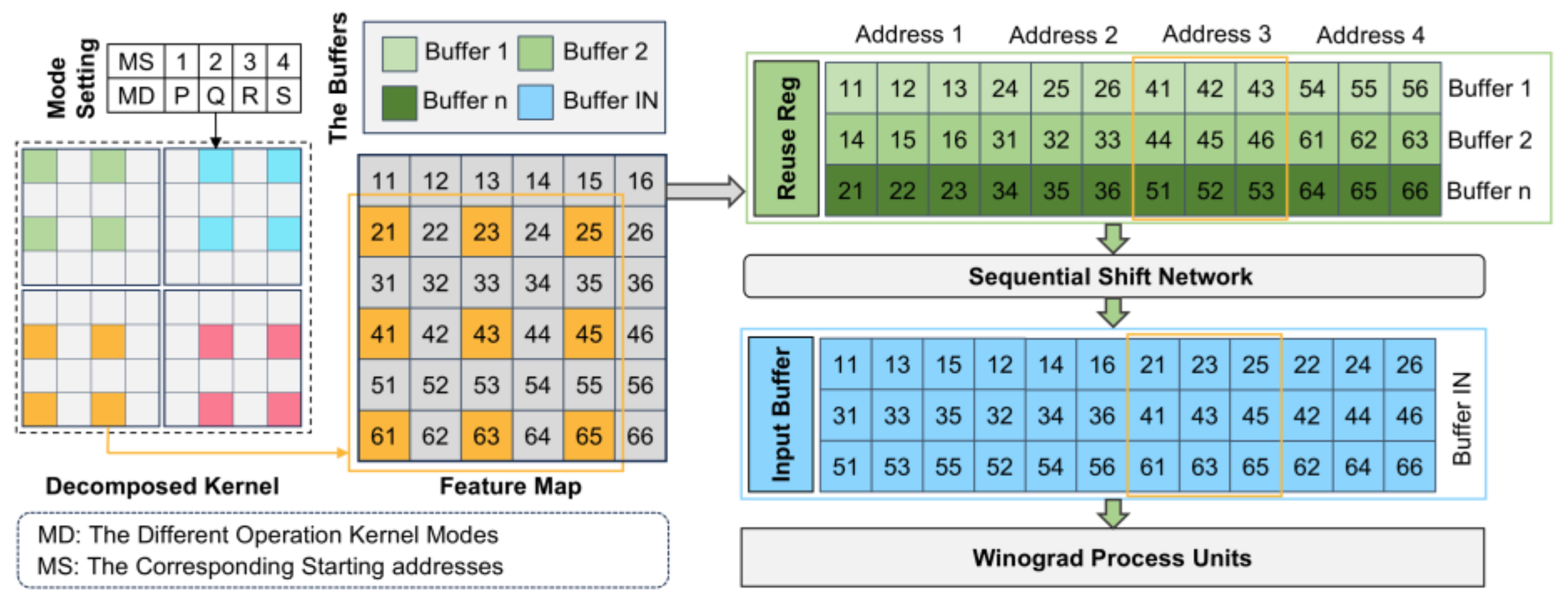
• To balance overall accelerator performance and power consumption, we present a design methodology for a reconfigurable Winograd processing system that effectively manages computational resources and power consumption. Additionally, by incorporating a preprocessing shift network and an address translation table, we achieve efficient data reuse between the accelerator system and storage blocks. This enhancement improves data access flexibility and efficiency while reducing system-induced latency;
• Implemented on the Xilinx XC7Z045 platform (AMD Xilinx, San Jose, CA, United States.), our design achieves an average throughput of 683.26 GOPS and a power efficiency of 74.51 GOPS/W.

The remainder of this paper is structured as follows: Section 3 reviews the Winograd algorithm and related work. Section 4 details our reconfigurable Winograd method with unified input tiling. Section 5 presents experimental discussions and comparisons. Section 6 concludes the paper.

3. Background

3.1. Winograd Algorithm

The Winograd algorithm, introduced by mathematician Shmuel Winograd in 1980, was initially applied in signal processing to reduce the computational complexity of impulse filters [25]. In 2016, the Winograd convolution algorithm was first used to accelerate Convolutional Neural Networks (CNNs) at the CVPR conference [14]. As an example, consider the one-dimensional Winograd convolution algorithm, where the output size of the convolution is denoted as m and the size of the convolution kernel is denoted as r, with the convolution computation represented as F (m, r). Let d represent the input data and g represent the convolution kernel data. The principles of the Winograd convolution algorithm are illustrated below using a specific set of computations.

$$\begin{array}{l}d={[d_0 d_1 d_2 d_3]}^T\\ g={[g_0 g_1 g_2]}^T\end{array}$$

(1)

For traditional convolution, the calculation process is as follows:

$$F(2,3)=\left[\begin{array}{ccc}{d}_0& d_1& d_2\\ d_1& d_2& d_3\end{array}\right]\left[\begin{array}{c}{g}_0\\ g_1\\ g_2\end{array}\right]=\left[\begin{array}{c}{r}_0\\ r_1\end{array}\right]$$

(2)

where r₀ and r₁ are defined as follows:

$$\begin{array}{l}{r}_0=(d_0·g_0)+(d_1·g_1)+(d_2·g_2)\\ r_1=(d_1·g_0)+(d_2·g_1)+(d_3·g_2)\end{array}$$

(3)

For Winograd convolution, the calculation process is as follows:

$$F(2,3)=\left[\begin{array}{ccc}{d}_0& d_1& d_2\\ d_1& d_2& d_3\end{array}\right]\left[\begin{array}{c}{g}_0\\ g_1\\ g_2\end{array}\right]=\left[\begin{array}{c}{m}_1+m_2+m_3\\ m_2-m_3-m_4\end{array}\right]$$

(4)

where

$$\begin{array}{ll}{m}_1=(d_0-d_2)g_0& m_4=(d_1-d_3)g_2\\ m_2=(d_1+d_2)\frac{g_0+g_1+g_2}{2}& m_3=(d_2-d_1)\frac{g_0-g_1+g_2}{2}\end{array}$$

(5)

Since the operations involving g₀, g₁, and g₂ need to be computed only once, the transformation of the convolution kernel can be disregarded in practical applications. In other words, the Winograd convolution requires only four multiplications and eight additions, while the traditional convolution algorithm involves six multiplications and four additions. The Winograd convolution thus saves 33% of multiplication operations, albeit at the cost of one additional addition. Given that the cost of implementing multiplication in hardware is substantially higher than that of addition, the Winograd convolution algorithm offers a hardware advantage over the traditional convolution algorithm. To further illustrate the two-dimensional Winograd convolution, we express the one-dimensional version with input size n, output size m, and kernel size r as a matrix multiplication.

$$Y=A^T\left[(Gg)\odot (B^{T}d)\right]$$

(6)

$$A=\left[\begin{array}{cc}1& 0\\ 1& 1\\ 1& -1\\ 0& -1\end{array}\right] {\mathrm{B}}^T=\left[\begin{array}{cccc}1& 0& -1& 0\\ 0& 1& 1& 0\\ 0& -1& 1& 0\\ 0& 1& 0& -1\end{array}\right] \mathrm{G}=\left[\begin{array}{ccc}1& 0& 0\\ \frac{1}{2}& \frac{1}{2}& \frac{1}{2}\\ \frac{1}{2}& -\frac{1}{2}& \frac{1}{2}\\ 0& 0& 1\end{array}\right]$$

(7)

In this context, A, G, and B represent the transformation matrices for the output feature map, convolution kernel, and input feature map, respectively. The expressions for each transformation matrix are provided in Equation (7). Y, d, and g correspond to the convolution output, input data, and kernel data, respectively. The symbol ⊙ denotes element-wise multiplication between tensors. The matrix form of the one-dimensional convolution F (4, 2, 3) is given in Equation (6).

For two-dimensional CNN computations, the result is obtained by applying the one-dimensional Winograd convolution twice in a nested fashion. As an example, consider the extension of the one-dimensional F (4, 2, 3) to two dimensions. Let the two-dimensional input image be denoted as g and the convolution kernel as d, as shown in Figure 1. First, the convolution operation between the input image and kernel is expanded into a matrix multiplication form. Then, as illustrated in Figure 1, the expanded matrices are partitioned according to the one-dimensional F (4, 2, 3). The resulting blocks are treated collectively, with the input matrix blocks labeled K0 to K3 and the expanded kernel matrix blocks labeled W0 to W2. It can be observed that the partitioned matrices retain the form of F (4, 2, 3), indicating that the two-dimensional Winograd convolution is derived by applying the one-dimensional F (4, 2, 3) convolution twice in a nested manner. Furthermore, in the two-dimensional Winograd convolution, the computational complexity of the matrix-vector multiplication operation is reduced to (m + r − 1)², representing a significant decrease compared to the traditional convolution, which requires m² + r² multiplications.

Similarly, the two-dimensional Winograd convolution is represented as $F\left(n_h\times n_{\omega }, m_h\times m_{\omega }, r_h\times r_{\omega }\right)$, where the input size is $n_h\times n_{\omega }$, the output size is $m_h\times m_{\omega }$, and the kernel size is $r_h\times r_{\omega }$. The mathematical expression for the two-dimensional Winograd convolution is provided in Equation (8).

$$Y={A_h}^T\left[(G_{h}g{G}_{\omega }^T)\odot (B_h^{T}d{B}_{\omega })\right]A_{\omega }$$

(8)

3.2. Computation Dataflow in CNN Training

This section provides an overview of the CNN training process [26]. To clearly describe the overall flow, the three process stages are divided into the following: forward propagation, backward propagation, and weight updates. The data flow in the convolutional layer during CNN training is illustrated in Figure 2. The data are categorized into weights (W), activations (A), errors (E), and gradients (G), with superscripts and subscripts denoting the layer indices, as outlined in

Table 1. The Illustration of CNN training parameters.

Parameter	Implication
L	The indices of the convolutional layer
h/w	The row or column indices of the feature map
H/W	The height or width of the feature map
Kh/kw	The row or column indices of the weight kernel
Kh/Kw	The height or width of the weight kernel
m/n	The indices of the input or output channel
M/N	The quantity of the input or output channel

, which provides a detailed definition of the relevant symbols. The computational processes at each stage of the convolutional layer are described below.

• Forward Propagation (FP): In the forward propagation stage of a neural network, the input is typically passed from one neuron to the next. The output of a layer is determined based on its input and the corresponding activation of the current layer ($A^L$). For example, in the CONV layer, as shown in Figure 2, the output value $A^L\left[n,h,w\right]$ is computed using the formula in Equation (9), where the current layer’s weight activations ($W^L$) are convolved with the activations from the previous layer ($A^{L-1}$).

  $$A^L[n,h,w]=\begin{array}{l}{\displaystyle \sum _{m=0}^{M-1}}{\displaystyle \sum _{k_h=0}^{K_h-1}}{\displaystyle \sum _{k_w=0}^{K_w-1}}{W}^L[n,m,k_h,k_w]\\ \times A^{L-1}[m,h+k_h,w+k_w]\end{array}$$

  (9)
• Backward Propagation (BP): In the backward propagation stage of a neural network, the computation process mirrors that of forward propagation. The key difference is that, during backward propagation, the kernel of the convolutional layer must be rotated by 180°. Additionally, the dimensions between the input and output channels are transformed. For the convolutional layer in the backward propagation stage, the output value $E^{L-1}\left[m,h,w\right]$ is obtained by convolving the activations of the current layer ($W^L$) with the errors from the same layer ($E^L$), as shown in Equation (10).

  $$E^{L-1}[m,h,w]=\begin{array}{l}{\displaystyle \sum _{n=0}^{M-1}}{\displaystyle \sum _{k_h=0}^{K_h-1}}{\displaystyle \sum _{k_w=0}^{K_w-1}}{W}^L[n,m,k_h,k_w]\\ \times E^L[m,h+K_h-1-k_h,w+K_w-1-k_h]\end{array}$$

  (10)
• Weight Gradient (WG): The weight gradient is the derivative of the loss with respect to the weights. For the CONV layer, the weight gradient ($G^L$) is obtained by convolving the activations from the previous layer ($A^{L-1}$) with the errors from the current layer ($E^L$), as shown in Equation (11).

  $$G^L[n,m,k_h,k_w]=\begin{array}{l}{\displaystyle \sum _{n=1}^{N-1}}{\displaystyle \sum _{h=1}^{H-1}}{\displaystyle \sum _{w=0}^{W-1}}{E}^L[n,h,w]\\ \times A^{L-1}[m,h+k_h,w+k_w]\end{array}$$

  (11)

3.3. The Layer-to-Layer Input-Uniform Decomposable Winograd Method

The introduction of the Decomposable Winograd Method (DWM) has significantly expanded the application range of the Winograd algorithm [27]. The literature suggests that when using a convolution kernel larger than 3 × 3 or a stride greater than 1, the kernel can be decomposed into several smaller kernels (each no larger than 3 × 3 with a stride of 1). The Winograd algorithm can then be applied to these smaller kernels. As a result, DWM can be utilized for convolution kernels of various sizes, addressing the major limitation of the Winograd algorithm and enabling its application in more general cases [11].

Although DWM broadens the applicability of the Winograd algorithm, its computation strategy, which standardizes the output size to 2 × 2, makes it difficult to implement on a unified processing unit. To overcome these issues, the literature introduces the Input-Aligned Decomposable Winograd Method (IA-DWM) [28], which resolves the issue of implementing DWM on a unified processing unit. However, IA-DWM lacks several important optimizations and features. For instance, IA-DWM employs traditional 4 × 4 block partitioning, resulting in a relatively low Winograd convolution multiplication saving ratio. To reduce resource consumption and improve throughput and energy efficiency, a larger block size is required, which is more suitable for deploying CNN accelerators on edge devices.

Moreover, the number and storage patterns of parallel buffers can be strategically organized by designing pre-stored reuse registers and optimizing the data retrieval sequence. This pre-read, reused data access pattern is particularly beneficial for small-kernel Decomposable Winograd Methods, as it maximizes memory utilization. To address these issues, a layer-to-layer 6 × 6 input-uniform Decomposable Winograd Method is proposed. The overall convolution process consists of five key steps:

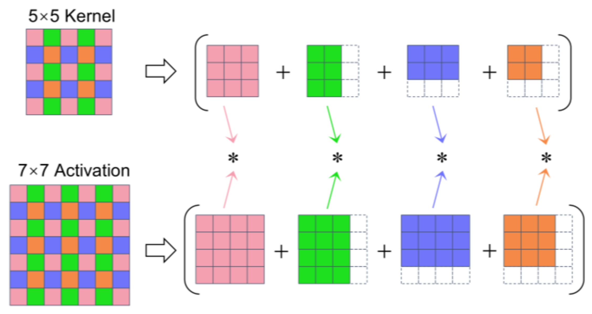
• Splitting: Large kernels are decomposed into smaller kernel tiles, each with a fixed stride of 1 and a size no greater than 3 × 3. Corresponding input tiles are also prepared. The kernel decomposition follows the stride-based convolution decomposition method proposed in [22], without requiring uniform padding of the kernels. Figure 3 illustrates the process of decomposing a 5 × 5 kernel with a stride of 2 into four smaller convolutions with a stride of 1, where the symbol “*” denotes the corresponding convolution operations;
• Transformation: The Winograd transformation matrix is applied to input tiles to obtain uniform 6 × 6 transformed matrices. This enhancement to uniform transformation focuses on increasing the input block size, thereby improving the multiplication saving ratio. The use of a 6 × 6 uniform input block, compared to smaller blocks, leads to better computational complexity and overall efficiency;
• Calculation: Do Element-wise multiplication and channel-wise summation, with these operations specifically implemented in the Winograd computation module and the Multiply-Accumulate (MAC) units designed in this paper;
• Inverse Transformation: The inverse transformation of the corresponding matrices is performed using the traditional Winograd algorithm, converting the intermediate results back to the spatial domain;
• Aggregation: The computed results from each part are summed, and the output tiles are rearranged to obtain the final result, which corresponds to the original convolution.

The basic operations and computational process of the 6 × 6-block DWM align with the two-dimensional Winograd convolution operations described in Section 3.1 and can similarly be expressed as $F\left(6\times 6,m_h\times m_{\omega },r_h\times r_{\omega }\right)$. However, the following constraints must be satisfied:

$$\left\{\begin{array}{l}{n}_h=n_{\omega }=6,\\ n_h=m_h+r_h-1,\\ n_{\omega }=m_{\omega }+r_{\omega }-1,\\ r_h\in [1,6],\\ r_{\omega }\in [1,6].\end{array}\right.$$

(12)

Based on the aforementioned constraints, the fundamental operations of the layer-to-layer DWM can be divided into two main processes:

• Decomposing convolution kernels larger than 3 × 3 or with a stride different from 1 into smaller unit convolutions;
• Performing the Winograd computation on the decomposed unit convolutions, as described in Equation (12). Specifically, when the convolution kernel size is 1 × 1, F (6 × 6, 6 × 6, 1 × 1) can be considered a special case, where the operation effectively reduces to element-wise matrix multiplication.

4. Architecture Design of Reconfigurable Accelerator

4.1. Overall Architecture

This section discusses the overall architecture of the layer-to-layer DWM-based CNN accelerator. Before discussing our overall design architecture, we selected four relevant CNN accelerator design architectures from a wide range of related works [15,29,30] and summarized their main features and differences in

Table 2. The main features and differences between the relevant design architectures.

Architecture Type	MAC Array	Characteristics	Drawbacks
GEMM-like	One-dimensional	High generality	Intensive computational complexity
Winograd-like	Two-dimensional	Small convolution kernels exhibit high computational efficiency	Large convolution kernels degrade computational performance
Winograd-GEMM-like	One or Two-dimensional	Dynamic optimal mode selection	Complex control logic introduces critical path delays
Reconfigurable-Winograd-like	Two-dimensional	Co-designed hardware and software ensure superior resource utilization	Transform kernel reconfiguration necessitates additional timing control

.

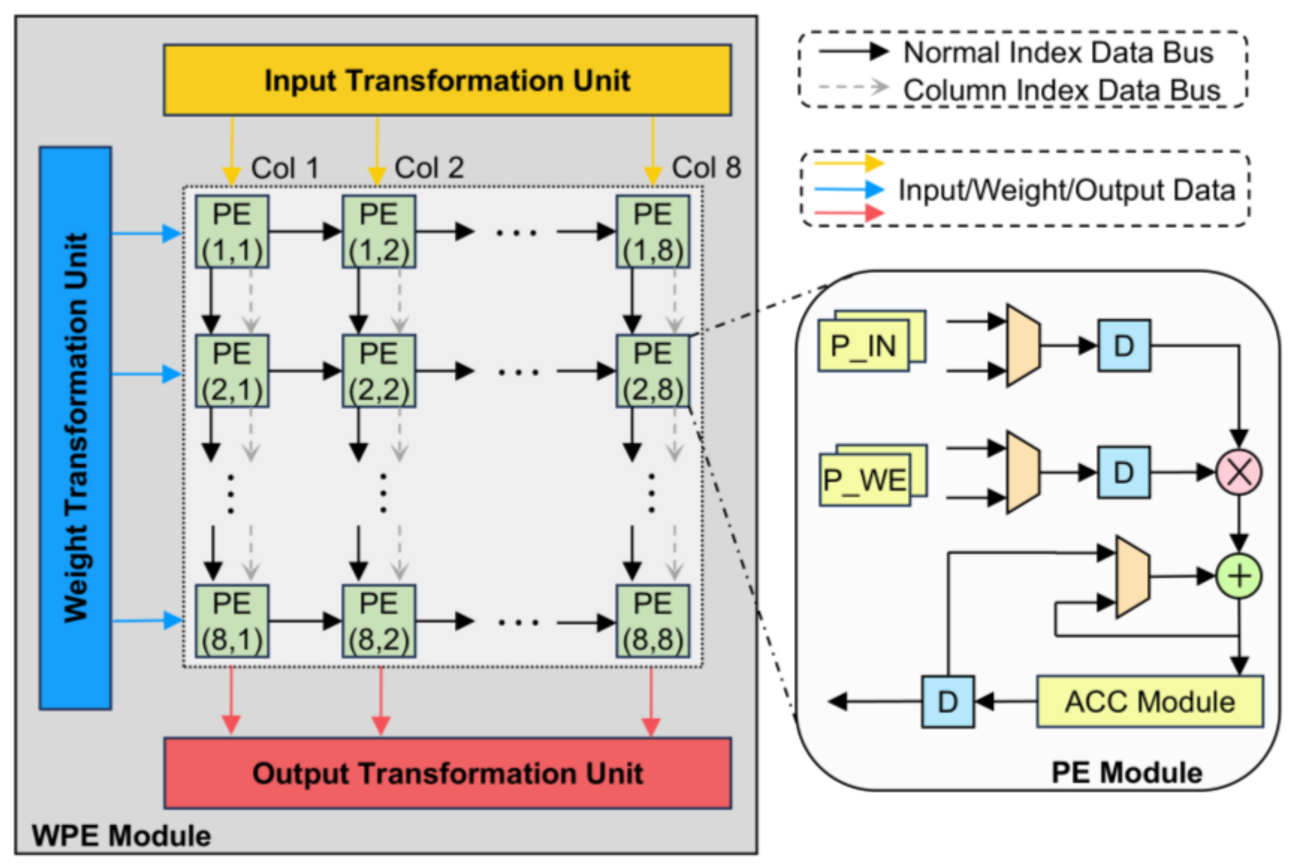
• These architectures differ in the data processing dimensions within the MAC unit, resulting in distinct convolution parallel execution schemes. The GEMM architecture uses a one-dimensional sequential design for its PE array, whereas the Winograd architecture typically employs a two-dimensional design. The hybrid Winograd architecture combines both dimensions, allowing for dynamic selection of CONV loop unrolling modes based on the kernel size. The reconfigurable Winograd architecture generally adopts a two-dimensional systolic array design. The differing array dimensions affect the execution order, partitioning, slicing, and unrolling operations during the CONV process;
• Compared to the GEMM, classic Winograd, and hybrid Winograd architectures, the reconfigurable Winograd architecture offers the greatest advantage through its ability to optimize across layers. This feature enhances hardware resource utilization via cross-layer pipelining reorganization and dynamic memory partitioning. Such software–hardware co-optimization is especially well suited for applications in edge heterogeneous computing environments. Consequently, we have chosen the reconfigurable Winograd architecture for our overall design framework.

Our accelerator framework leverages the DWM architecture, incorporating several optimizations to enhance performance and reduce resource usage. The structure of the accelerator, as illustrated in Figure 4, consists of the main controller unit, layer-to-layer transformation unit, Winograd Process Unit (WPU), data access unit, Auxiliary Processing Unit (APU), data cache unit, and Advanced Extensible Interface communication unit (AXI). Data exchange between on-chip and off-chip memory is managed by DDR, following the AXI bus protocol.

The main controller coordinates the input and output data flows, configures the read and write operations for weight data, and oversees the entire computation process. To improve computational efficiency, a layer-to-layer input transformation structure is designed to enhance the multiplication savings ratio in Winograd convolution. Flexible cache configurations are also implemented to accommodate various data access patterns, ensuring efficient data flow to the PE units. The WPU, as the core computational module, is primarily responsible for performing convolution (CONV) layer operations. A novel structural design of the PE array reduces trigger power consumption. The APU accumulates channel data after computation in the PE units, caches it, and subsequently performs non-convolution operations to update the weights. Finally, the results are transferred via the AXI bus to the external DRAM for subsequent input data processing.

4.2. Design of Layer-to-Layer Transformation Units

The Winograd algorithm is an efficient optimization technique for smaller convolutions. However, in neural network computations, the input feature map is typically large, necessitating block-based processing followed by individual Winograd convolution computations. The choice of block size directly influences the complexity of the input-output transformation coefficient matrices and the algorithm’s acceleration performance. As block size increases, the Winograd convolution achieves a higher multiplication savings ratio. However, this also results in larger ranges of transformation matrix coefficients, increasing the complexity and precision requirements for hardware circuit design. Larger block sizes are not always advantageous; block sizes greater than 8 × 8 lead to significant precision loss during hardware implementation, which can negatively impact the prediction accuracy of the CNN. For odd block sizes, input feature maps require additional processing such as static padding, dynamic overlapping, or dynamic border removal. Therefore, even block sizes are often preferred in practical applications.

Considering these factors, our design adopts a uniform 6 × 6 block method. Most existing designs, such as the IA-DWM architecture [28], use a 4 × 4 block size due to the simplicity of hardware implementation for transformation matrix coefficients. As shown in Equation (13), the transformation matrices for the input and output feature maps contain only the coefficients 0, 1, and −1, allowing matrix transformations to be performed using addition operations. The fractional values in the convolution kernel transformation matrix G can be handled through bit-shifting. In our proposed 6 × 6 block method, the transformation matrix is shown in Equation (14). Although this introduces more complex coefficients, optimization techniques enable the constant coefficients in the input and output transformation matrices to be replaced by a combination of bit shifts. For instance, 5 can be represented as 2² + 1.

$$A^T=\left[\begin{array}{cccc}1& 1& 1& 0\\ 0& 1& -1& 1\end{array}\right] {\mathrm{B}}^T=\left[\begin{array}{cccc}1& 0& -1& 0\\ 0& 1& 1& 0\\ 0& -1& 1& 0\\ 0& 1& 0& -1\end{array}\right] \mathrm{G}=\left[\begin{array}{ccc}1& 0& 0\\ \frac{1}{2}& \frac{1}{2}& \frac{1}{2}\\ \frac{1}{2}& -\frac{1}{2}& \frac{1}{2}\\ 0& 0& 0\end{array}\right]$$

(13)

$$A^T=\left[\begin{array}{cccccc}1& 1& 1& 1& 1& 0\\ 0& 1& -1& 2& -2& 0\\ 0& 1& 1& 4& 4& 0\\ 0& 1& -1& 8& -8& 1\end{array}\right] {\mathrm{B}}^T=\left[\begin{array}{cccccc}4& 0& -5& 0& 1& 0\\ 0& -4& -4& 1& 1& 0\\ 0& 4& -4& -1& 1& 0\\ 0& -2& -1& 2& 1& 0\\ 0& 2& -1& -2& 1& 0\\ 0& 4& 0& -5& 0& 1\end{array}\right] \mathrm{G}=\left[\begin{array}{ccc}\frac{1}{4}& 0& 0\\ -\frac{1}{6}& -\frac{1}{6}& -\frac{1}{6}\\ -\frac{1}{6}& \frac{1}{6}& \frac{1}{6}\\ \frac{1}{24}& \frac{1}{12}& \frac{1}{6}\\ \frac{1}{24}& -\frac{1}{12}& \frac{1}{6}\\ 0& 0& 1\end{array}\right]$$

(14)

Since the multiplication of constants in the convolution kernel transformation matrix G can become complex and difficult to maintain precision, and considering that the convolution kernels remain fixed during the neural network inference phase, we preprocess the convolution kernel transformation off-chip.

Table 3. Comparison of different segmentation sizes of input feature map (N × N).

Tile Size	Segmentation Size	Multiplication Complexity	Addition Complexity
4 × 4	(N/2)2	16× (N/2)2	56× (N/2)2
6 × 6	(N/4)2	32× (N/2)2	276× (N/2)2

compares the computational impact of the 4 × 4 and 6 × 6 block methods. Here, C represents the feature map’s length and width. For the same input image, the number of blocks in the 6 × 6 method is one-quarter of that in the 4 × 4 method. The multiplication operations in the 6 × 6 method account for 56.25% of those in the 4 × 4 method, while the addition operations are 1.23 times greater in the 6 × 6 method. This demonstrates that the 6 × 6 block method improves the Winograd convolution multiplication saving ratio, leading to better computational efficiency and overall performance.

The input feature map transformation, based on the two-dimensional Winograd transformation Equation (8), is expressed as $U=B^{T}HB$, where B is a constant coefficient transformation matrix related to the block size of the input feature map, and H represents the input feature map blocks. Equation (15) provides the direct computation formula for the left transformation, while the right transformation uses the same coefficients as the left. Existing designs encounter the following issues when handling the input feature map transformation:

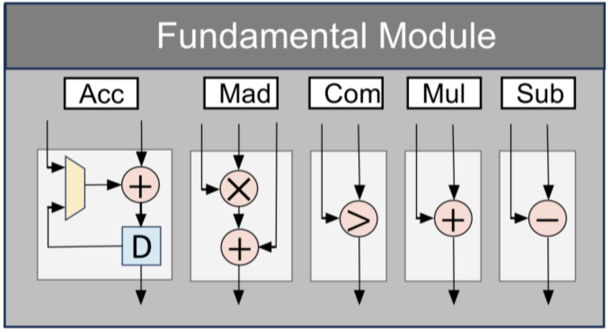
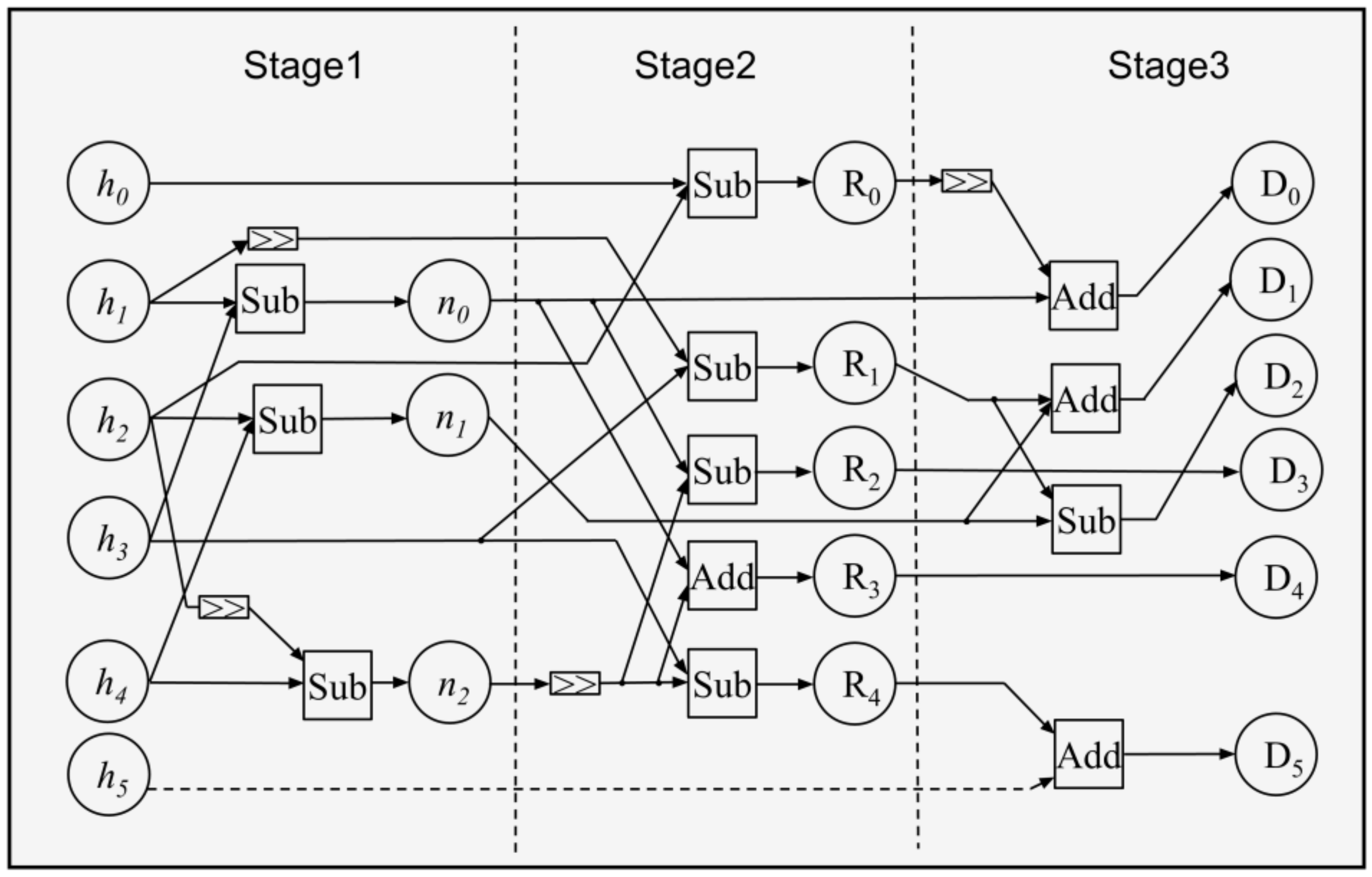
• The computation of U = B^T HB requires completing the U = B^T HB calculation before proceeding to the subsequent multiplication with the matrix B. This sequential processing can result in the addition delay exceeding the matrix dot product unit delay, thereby degrading the overall performance of the accelerator;
• The input transformation matrix involves lengthy chain additions, which can adversely impact the system clock frequency. Additionally, the intermediate results from the addition computation contain reusable components, leading to significant redundant calculations when computed directly.

To address these issues, we propose a layer-to-layer input transformation computation structure. In this transformation, we define the following expressions: $N_{m0}=-h_{2m}+h_{4m}$, $N_{m1}=-4h_{2m}+h_{4m}$, and $N_{m2}=h_{1m}-h_{3m}$. This modifies the left transformation computation formula to Equation (16). This method splits and recombines the calculations, enabling constant multiplications to be implemented via bit shifts. By reusing the results of $N_{m0}$, $N_{m1}$, and $N_{m2}$, the addition computation for a single channel is reduced from 192 operations to 156, achieving an 18.75% reduction. Compared to directly computing the long-chain additions, this approach improves the system’s clock frequency and enhances pipeline computation efficiency.

Additionally, to better design the hardware circuit for the layer-to-layer computation structure, we divide the design into five basic operations, each with a corresponding hardware circuit. As shown in Figure 5, these operations are “Accumulation (Acc)”, “Multiply-Addition (Mad)”, “Subtraction (Sub)”, “Comparison (Com)”, and “Signed Multiplication (Mul)”. The Sub operation is based on a full subtractor, while the Signed-Mult operation utilizes a signed multiplier.

$$H=\left[\begin{array}{c}{h}_{0m}\\ h_{1m}\\ h_{2m}\\ h_{3m}\\ h_{4m}\\ h_{5m}\end{array}\right] m\in [0,5] B^T·H=\left[\begin{array}{c}4h_{0m}-5h_{2m}+h_{4m}\\ -4h_{1m}-4h_{2m}+3h_{3m}+h_{4m}\\ 4h_{1m}-4h_{2m}-h_{3m}+h_{4m}\\ -2h_{1m}-h_{2m}+2h_{3m}+h_{4m}\\ 2h_{1m}-h_{2m}-2h_{3m}+h_{4m}\\ 4h_{2m}-5h_{4m}+h_{5m}\end{array}\right] \mathrm{m}\in [0,5]$$

(15)

$$B^T·H=\left[\begin{array}{c}4h_{0m}-4h_{2m}+N_{m0}\\ -4h_{1m}+h_{3m}+N_{m1}\\ 4h_{1m}-h_{3m}+N_{m1}\\ N_{m0}-2N_{m2}\\ N_{m0}+2N_{m2}\\ 4N_{m0}-h_{3m}+h_{5m}\end{array}\right] m\in [0,5]$$

(16)

Since the right transformation of the input feature map is symmetric to the left transformation and shares the same coefficient matrix, the computation circuit for both transformations is identical. Therefore, a single layer-to-layer computation circuit can be used for both transformations. The structure of the layer-to-layer left transformation circuit for the input layer is shown in Figure 6. Each computation stage consists of basic two-input operations, and the overall process is divided into three pipelined stages. In Stage 1, we design a data reuse phase; Stage 2 functions as a temporary storage phase for the computations, while Stage 3 is the accumulation phase where the results are summed. Compared to directly computing the long-chain additions, our design enables a higher system clock frequency, and the pipelined approach significantly improves computational efficiency. We have developed a unified two-dimensional transformation module, which contains six parallel, cascaded one-dimensional transformation modules. These modules convert cached one-dimensional data into two-dimensional data, which is then sent to the input transformation and weight transformation modules for transformation before being broadcast to the Winograd Processing Elements for element-wise dot product operations.

4.3. Architecture of Winograd Processing Element

Structure of WPE Array: The PE array module is a critical component of CNN accelerators. In CNN models, over 90% of arithmetic operations and weight parameters originate from convolutional layers and matrix multiplication. To fully utilize the bus resources between Winograd Processing Elements (WPEs) in both spatial and temporal dimensions, we have designed a reconfigurable Winograd PE array structure, as shown in Figure 7. In the classic WPE array design, if Q is the total number of WPEs in the array, the corresponding total bus resource usage is given by:

$$B\_Trad=Q\left(Q+1\right)/2\left(Q+P\_IN\right)$$

(17)

As shown in Figure 7, in our improved array structure, we arrange the WPEs in a matrix-like format with c rows and m columns, where $Q=c\times m$. Here, $\left(i,j\right)$ represents the pulse array index, with i as the row index and j as the column index. In our architecture, the bus resources for each pair of adjacent WPEs in the same row are the same as in the traditional pulse array. When the pulse array traverses from the current row to the next, the row index i is reset to 1. This significantly reduces the total bus output resource usage.

Additionally, extra buses are introduced between some adjacent WPEs in different columns to skip portions of the computation data flow. Therefore, the total bus resource usage in our design is given by the following:

$$B\_Nov=Col\times m+D$$

(18)

where Col is the total number of column buses, and D is the number of output buses in the last row. The equations for Col and D are as follows:

$$Col=n\left(n+1\right)/\left(2\left(n+P\_IN\right)\right), D=\left(m\left(m+1\right)\right)/\left(2\times n\times P\_IN\right)$$

(19)

With 64 WPEs forming the PE array, our design reduces the number of output bus ports by 34% compared to previous designs, thereby reducing the total power consumption of the flip-flops.

Furthermore, we introduce multi-stage parallel pipelining, with all data passing through a transformation unit and entering the WPE array in matrix form. The WPE array retrieves data from eight different channels and sequentially broadcasts the data to different WPEs in the order of $\left(i,j+1\right)$. The data are then accumulated within the WPEs and output as a data stream, which is stored in the output cache module.

Architecture of PE: As shown in the right part of Figure 7, the basic structure of the PE consists of P_IN MAC units and multiple multiplexers. These multiplexers configure the WPE for various layer-specific operations. Each MAC unit processes data streams of size P_WE, extracting fixed-weight arrays from the input and weight feature providers and performing element-wise accumulation. Here, P_IN and P_WE represent the length and size of the feature maps from the Feature Provider and Weight Provider units, respectively. The computational outputs of all MAC units are simultaneously stored in the local output buffer. Upon completing a full iteration of convolution, the PE transfers the data stream from the buffer to the output cache.

4.4. Data and Memory Allocation

In Section 3, we introduced the decomposable Winograd method, which decomposes large convolution kernels or convolution kernels with non-fixed strides into several smaller convolution kernels with a stride of 1 [27]. These smaller kernels are then processed using conventional convolution operations. Conventional convolution involves sliding a fixed-size kernel across the input feature map, where at each position, the corresponding elements of the kernel and input feature map are multiplied and summed. However, unlike conventional convolution, the DWM for neural network training must address the issue of data access for convolution kernels of varying sizes on the input feature map. Therefore, it is essential to establish corresponding data access patterns for convolution kernels of different sizes to improve data processing efficiency and enhance the utilization of PEs. To solve this problem, we employ a shift network in the preprocessing buffer for data access management.

Feature Provider: As shown in Figure 8, the mapping of different kernel sizes after decomposition can be represented by a corresponding configuration table, where the starting address MS guides the address generation for the different kernel mapping modes, and MD represents the various working modes of the kernel mapping. To improve the computational efficiency of kernels for different working modes and ensure optimal utilization of PEs, we design a “Reuse Loader” preprocessing buffer. This buffer allows data that has been pre-read to be reused by subsequent inputs, thus enhancing on-chip memory access efficiency.

For data that can be reused or needs to be repeatedly read during computation, we pre-store these data in the “Reuse Loader” upon its first read to maximize data reuse and minimize the access load on the on-chip storage. Subsequent accesses are then managed with appropriate data shifting and alignment in the input buffer, based on the specific working mode. Due to constraints in data access modes, the data in the buffer needs to be cascaded with adjacent pre-stored data to ensure the correct generation of data streams for the shift registers. Additionally, we define a proper order for reading data from the buffer to avoid conflicts caused by redundant on-chip memory accesses. The input buffer is composed of 16 independent on-chip memory units, with each entry in the buffer corresponding to 8 input channels. This setup ensures that each row of the input buffer can store a 6 × 6 tile.

Weight Provider: The weight buffer consists of 32 independent on-chip memory units, with each memory unit containing entries that store eight input channels and eight output channels. The buffer is scaled to match the Processing Element array and is used to provide the weight parameters required by the convolution layer during different training phases: forward propagation, back propagation, and weight gradient stages. Similar to the feature provider, the weight provider is configured with different access modes to handle the data flow for each of these stages.

Auxiliary Process Unit: We have designed a dedicated Auxiliary Processing Unit (APU) to manage all non-convolution operations in the accelerator. The APU consists of modules for channel accumulation, max pooling, quantization, activation, and fully connected layers. Each local module within the APU comprises basic functional units, including a master controller, shift registers, basic registers, comparators, and accumulators. The corresponding hardware circuits for these components are shown in Figure 8. The master controller oversees APU operations by managing on-chip and off-chip cache data, the number of computation layers, and input/output feature parameters and weight updates through enabled signals. Furthermore, by deploying independent computation units and data flow control, the APU enables parallel pipelined computation across its local modules, thereby enhancing computational efficiency.

5. Discussion

5.1. Experimental Setup

Our accelerator is designed using Verilog HDL and compiled and synthesized with the Xilinx Vivado Design Suite 2021.2. The Xilinx XC7Z045 platform was selected for our experiments, featuring 218 K lookup tables, 343 K flip-flops, 545 BRAM blocks, 900 Digital Signal Processors (DSPs), and two 4 GB DDR3 DRAM modules for off-chip memory to store weight parameters. The accelerator operates at a frequency of 150 MHZ. In [31], a detailed analysis of the 8-bit PINT data format quantization strategy is presented, with FP32 as the reference baseline. The weight, input feature map data, and output feature map data are all represented in the 8-bit PINT format, resulting in less than 0.4% accuracy degradation for VGG16 and ResNet18. Furthermore, the 8-bit PINT format reduces memory resource usage, simplifying the design of the basic computation units. As a result, this novel data format is employed for CNN training in this study. In the following analysis, we use “MACs” and “PEs” as abstract terms referring to theoretical hardware components capable of multiplication and accumulation operations, rather than specific elements such as LUTs or DSPs used in the accelerator design.

5.2. Experiment Results Analysis

In this section, we evaluate the performance of our accelerator on mainstream CNN architectures, specifically VGG-16 [32] and ResNet-18 [33]. The accelerator is configured to use the ResNet-18 and VGG-16 architectures for image classification on the ImageNet dataset, with an input size of 224 × 224 pixels. The throughput performance of the accelerator is estimated based on the total number of operations and the overall latency incurred by executing the convolutional layers. This total latency includes computation time, access time between DRAM and on-chip buffers, and the time required for reading and writing input, output, and weight data. The power consumption of the accelerator is evaluated using the Xilinx Vivado 2021.2 Power Analysis Tool.

Figure 9 and Figure 10 illustrate the training waiting latency and overall MACs utilization across different layers during various training stages for both VGG-16 and ResNet-18. In the ResNet-18 network, certain layers (e.g., conv 1.1.1, conv 3.1.3) exhibit lower MAC utilization, which can be attributed to the network architecture and cache access design. For example, the first layer of ResNet-18 has only 3 input channels. This limited number of channels leads to inefficient division of input features into 6 × 6 input tiles, resulting in incomplete MAC mapping and reduced utilization. Moreover, due to the memory bandwidth limitation of 2.4 GB/s in the Zynq 7000 series (Xilinx XC7Z045. AMD Xilinx, San Jose, CA, United States.) and hardware resource constraints, the access time between off-chip DRAM and on-chip buffers is longer compared to using BRAM for data access. This results in increased processing time for small convolution layers and non-convolution layers.

Furthermore, in the memory design described in Section 4.4, we implemented a pre-stored cache shift mechanism to enhance the flexibility of data access patterns and improve data reuse. This design increases data reuse for large convolution layers, which in turn reduces MAC utilization in certain smaller convolution layers. However, since these specific layers constitute a relatively small proportion of the overall computation in the ResNet-18 network, the average MAC utilization remains at 90%, with an average throughput of 674.46 GOPS. In the VGG-16 network, the average MAC utilization is 85%, with an average throughput of 665.74 GOPS.

5.3. Comparison with Other Works

Due to the differences in experimental platforms chosen in the related works, the throughput performance and processing capabilities naturally differ based on the hardware resources of each platform. To better reflect the impact of platform design on CNN inference acceleration performance, we adopted a normalization method for key performance metrics [34], using throughput normalization metrics such as DSP Efficiency (GOPS/DSP) and power efficiency (GOPS/W) for cross-platform efficiency comparison.

We compared the proposed accelerator design with existing works, and the results are summarized in

Table 4. Comparison with existing CNN FPGA works.

	2019 [15]	2020 [13]	2022 [18]	2022 [17]	2023 [19]	2023 [21]	2024 [20]	Ours
Model	VGG-16	ResNet-18	VGG-16	VGG-16	VGG-16	ResNet-18	VGG-16	VGG-16	ResNet-18
Platform	VX690T	XC7Z045	XC7Z045	VX980T	XCVU9P	XC7Z045	XCVU9P	XC7Z045
Freq (MHz)	200	200	150	150	200	200	430	150
Precision	16-bit	8-bit	8-bit	8/16-bit	8-bit	8-bit	8-bit	8-bit
LUT	468.0 K	100.2 K	NA	335.0	NA	17.4 K	93.0 K	114.7 K
BRAMs	1465	NA	545	1492	NA	112	336	272
DSPs	1436	818	900	3395	384	182	576	786
Power (W)	17.30	7.31	NA	14.36	NA	0.62	37.60	9.03	9.17
Throughput (GOPS)	407.23	124.90	374.98	1000.00	402.00	88.91	711.00	665.38	683.26
DSP Eff. (GOPS/DSPs)	0.28	0.15	0.42	0.29	1.05	0.49	1.23	0.85	0.87
Power Eff. (GOPS/W)	23.53	17.09	NA	69.64	NA	143.41	18.91	72.84	74.51

. Ref. [15] proposed a unified accelerator architecture for the Winograd and GEMM algorithms in the PE array, enabling parallel computation of all CNN layers using FPGA hardware. However, it is constrained by kernel size and stride, leading to excessive resource usage. In contrast, our design is not limited by kernel size and achieves a 1.63× performance improvement for VGG-16 and a 3.13× increase in energy efficiency (Power Efficiency). Clearly, our design outperforms others in both performance and PE utilization.

For VGG-16, the work in [20] uses the general Winograd F (4, 3) as a computation unit to process 3 × 3 and 1 × 1 convolutions for improved performance. Compared to our improved DWM, Ref. [20] provides a 1.06× performance improvement at a clock frequency of 430 MHz, but this comes at the cost of a significant increase in power consumption, resulting in a reduction in power efficiency by approximately four times. This lower energy efficiency makes it less favorable for edge applications.

In the case of VGG-16, Ref. [17] designed a layer-specific pipelining strategy for each convolution layer, resulting in improved performance. However, their DSP efficiency is only one-third of what our design achieves. Ref. [19] proposed a hardware–software co-designed accelerator, which, due to its integration of both software and hardware, introduces additional latency, limiting the network’s performance. Despite a 23% improvement in DSP efficiency over our design, their performance is 65% lower than ours. Ref. [18] deployed VGG-16 on a low-cost FPGA for the first time, introducing a block convolution design that eliminates the need for external DRAM for data caching, thus reducing latency. However, due to their high BRAM usage, their DSP efficiency is significantly lower than ours.

For the ResNet-18 network, which primarily consists of 3 × 3 and 1 × 1 convolutions, the Winograd and GEMM algorithms are efficient methods for such architectures. Our improved DWM outperforms the general Winograd design in [13] by 5.4× in performance and 4.36× in energy efficiency. The GEMM-based design in [21] uses fewer resources and consumes less power, achieving an energy efficiency of 143.41 GOPS/W, which is 1.91 times higher than our design. However, our accelerator’s performance is 7.68× that of [21], while also providing a 1.77× improvement in DSP efficiency.

In summary, through comparison and evaluation with similar works, our accelerator achieves a better balance between overall performance and energy efficiency. Compared to existing solutions, we have made the following key improvements. First, we optimized the DWM by introducing a 6 × 6 input block partitioning scheme and a layer-to-layer input transformation design. This unification of the input, weight, and output transformation units enhances the scalability of the Winograd algorithm. Additionally, our improved DWM can handle kernels with varying sizes and strides simultaneously. We also introduced a preprocessing shift network based on kernel size, enabling flexible selection of Winograd’s basic computation units and matching parameters for decomposed kernels. This approach leads to higher data access efficiency and improved performance.

6. Conclusions

In this paper, we present a CNN accelerator that utilizes a layer-to-layer Decomposable Winograd Method to reduce computational redundancy in input-output transformations, thereby expanding the applicability of the Winograd algorithm. Additionally, we introduce a preprocessing shift network technique that selects the optimal data access pattern and Winograd computation unit for each layer based on kernel splitting rules. This approach enhances both the flexibility and efficiency of data access. The implementation experimental evaluations implemented on VGG-16 and ResNet-18 demonstrate that our design achieves average throughputs of 665.38 GOPS/DSP and 683.26 GOPS/DSP, and energy efficiencies of 72.84 GOPS/W and 74.51 GOPS/W, respectively. Compared to existing implementations, these results represent improvements in throughput, DSP efficiency, and energy efficiency by factors of 7.68×, 5.8×, and 3.85×, respectively, delivering higher speeds and better energy efficiency. While our design shows promising performance, further investigation into hybrid input DWM could expand the scope of DWM applications and enhance the flexibility of the Winograd algorithm in CNN accelerators.

References

1. Nguyen, D.T.; Nguyen, T.N.; Kim, H.; Lee, H.-J. A High-Throughput and Power-Efficient FPGA Implementation of YOLO CNN for Object Detection. IEEE Trans. Very Large Scale Integr. (VLSI) Syst. 2019, 27, 1861–1873. [Google Scholar] [CrossRef]
2. Ndikumana, A.; Tran, N.H.; Kim, D.H.; Kim, K.T.; Hong, C.S. Deep Learning Based Caching for Self-Driving Cars in Multi-Access Edge Computing. IEEE Trans. Intell. Transp. Syst. 2021, 22, 2862–2877. [Google Scholar] [CrossRef]
3. Arefin, M.; Hossen, K.M.; Uddin, M.N. Natural Language Query to SQL Conversion Using Machine Learning Approach. In Proceedings of the 2021 3rd International Conference on Sustainable Technologies for Industry 4.0 (STI), Dhaka, Bangladesh, 18–19 December 2021; pp. 1–6. [Google Scholar]
4. Krizhevsky, A.; Sutskever, I.; Hinton, G.E. ImageNet Classification with Deep Convolutional Neural Networks. Commun. ACM 2017, 60, 84–90. [Google Scholar] [CrossRef]
5. Kim, N.J.; Kim, H. FP-AGL: Filter Pruning with Adaptive Gradient Learning for Accelerating Deep Convolutional Neural Networks. IEEE Trans. Multimed. 2023, 25, 5279–5290. [Google Scholar] [CrossRef]
6. Li, T.; Sahu, A.K.; Talwalkar, A.; Smith, V. Federated Learning: Challenges, Methods, and Future Directions. IEEE Signal Process. Mag. 2020, 37, 50–60. [Google Scholar] [CrossRef]
7. Choquette, J.; Gandhi, W.; Giroux, O.; Stam, N.; Krashinsky, R. NVIDIA A100 Tensor Core GPU: Performance and Innovation. IEEE Micro 2021, 41, 29–35. [Google Scholar] [CrossRef]
8. Syed, R.T.; Andjelkovic, M.; Ulbricht, M.; Krstic, M. Towards Reconfigurable CNN Accelerator for FPGA Implementation. IEEE Trans. Circuits Syst. II Express Briefs 2023, 70, 1249–1253. [Google Scholar] [CrossRef]
9. Zhao, Z.; Cao, R.; Un, K.-F.; Yu, W.-H.; Mak, P.-I.; Martins, R.P. An FPGA-Based Transformer Accelerator Using Output Block Stationary Dataflow for Object Recognition Applications. IEEE Trans. Circuits Syst. II Express Briefs 2023, 70, 281–285. [Google Scholar] [CrossRef]
10. Chun, D.; Choi, J.; Lee, H.-J.; Kim, H. CP-CNN: Computational Parallelization of CNN-Based Object Detectors in Heterogeneous Embedded Systems for Autonomous Driving. IEEE Access 2023, 11, 52812–52823. [Google Scholar] [CrossRef]
11. Habib, G.; Qureshi, S. Optimization and Acceleration of Convolutional Neural Networks: A Survey. J. King Saud Univ.—Comput. Inf. Sci. 2022, 34, 4244–4268. [Google Scholar] [CrossRef]
12. Basalama, S.; Sohrabizadeh, A.; Wang, J.; Guo, L.; Cong, J. FlexCNN: An End-to-end Framework for Composing CNN Accelerators on FPGA. ACM Trans. Reconfigurable Technol. Syst. 2023, 16, 1–32. [Google Scholar] [CrossRef]
13. Liang, Y.; Lu, L.; Xiao, Q.; Yan, S. Evaluating Fast Algorithms for Convolutional Neural Networks on FPGAs. IEEE Trans. Comput. Aided Des. Integr. Circuits Syst. 2020, 39, 857–870. [Google Scholar] [CrossRef]
14. Lavin, A.; Gray, S. Fast Algorithms for Convolutional Neural Networks. In Proceedings of the IEEE Conference on Computer Vision and Pattern Recognition (CVPR), Las Vegas, NV, USA, 27–30 June 2016; pp. 4013–4021. [Google Scholar]
15. Kala, S.; Jose, B.R.; Mathew, J.; Nalesh, S. High-Performance CNN Accelerator on FPGA Using Unified Winograd-GEMM Architecture. IEEE Trans. Very Large Scale Integr. (VLSI) Syst. 2019, 27, 2816–2828. [Google Scholar] [CrossRef]
16. Mahale, G.; Udupa, P.; Chandrasekharan, K.K.; Lee, S. WinDConv: A Fused Datapath CNN Accelerator for Power-Efficient Edge Devices. IEEE Trans. Comput. Aided Des. Integr. Circuits Syst. 2020, 39, 4278–4289. [Google Scholar] [CrossRef]
17. Huang, W.; Wu, H.; Chen, Q.; Luo, C.; Zeng, S.; Li, T.; Huang, Y. FPGA-Based High-Throughput CNN Hardware Accelerator With High Computing Resource Utilization Ratio. IEEE Trans. Neural Netw. Learn. Syst. 2022, 33, 4069–4083. [Google Scholar] [CrossRef]
18. Li, G.; Liu, Z.; Li, F.; Cheng, J. Block Convolution: Toward Memory-Efficient Inference of Large-Scale CNNs on FPGA. IEEE Trans. Comput. Aided Des. Integr. Circuits Syst. 2022, 41, 1436–1447. [Google Scholar] [CrossRef]
19. Kim, D.; Jeong, S.; Kim, J.Y. Agamotto: A Performance Optimization Framework for CNN Accelerator With Row Stationary Dataflow. IEEE Trans. Circuits Syst. I Regul. Pap. 2023, 70, 2487–2496. [Google Scholar] [CrossRef]
20. Yang, C.; Yang, Y.; Meng, Y.; Huo, K.; Xiang, S.; Wang, J.; Geng, L. Flexible and Efficient Convolutional Acceleration on Unified Hardware Using the Two-Stage Splitting Method and Layer-Adaptive Allocation of 1-D/2-D Winograd Units. IEEE Trans. Comput. Aided Des. Integr. Circuits Syst. 2024, 43, 919–932. [Google Scholar] [CrossRef]
21. See, J.-C.; Ng, H.-F.; Tan, H.-K.; Chang, J.-J.; Mok, K.-M.; Lee, W.-K.; Lin, C.-Y. Cryptensor: A Resource-Shared Co-Processor to Accelerate Convolutional Neural Network and Polynomial Convolution. IEEE Trans. Comput. Aided Des. Integr. Circuits Syst. 2023, 42, 4735–4748. [Google Scholar] [CrossRef]
22. Yang, C.; Wang, Y.; Wang, X.; Geng, L. A Stride-Based Convolution Decomposition Method to Stretch CNN Acceleration Algorithms for Efficient and Flexible Hardware Implementation. IEEE Trans. Circuits Syst. I Regul. Pap. 2020, 67, 3007–3020. [Google Scholar] [CrossRef]
23. Cheng, C.; Parhi, K.K. Fast 2D Convolution Algorithms for Convolutional Neural Networks. IEEE Trans. Circuits Syst. I Regul. Pap. 2020, 67, 1678–1691. [Google Scholar] [CrossRef]
24. Pan, J.; Chen, D. Accelerate Non-Unit Stride Convolutions with Winograd Algorithms. In Proceedings of the Proceedings of the 26th Asia and South Pacific Design Automation Conference, Tokyo, Japan, 18–21 January 2021; Association for Computing Machinery: New York, NY, USA, 2021; pp. 358–364. [Google Scholar]
25. Winograd, S. Arithmetic Complexity of Computations; SIAM: Delhi, India, 1980; ISBN 978-0-89871-163-9. [Google Scholar]
26. Alzubaidi, L.; Zhang, J.; Humaidi, A.J.; Al-Dujaili, A.; Duan, Y.; Al-Shamma, O.; Santamaría, J.; Fadhel, M.A.; Al-Amidie, M.; Farhan, L. Review of Deep Learning: Concepts, CNN Architectures, Challenges, Applications, Future Directions. J. Big Data 2021, 8, 53. [Google Scholar] [CrossRef] [PubMed]
27. Huang, D.; Zhang, X.; Zhang, R.; Zhi, T.; He, D.; Guo, J.; Liu, C.; Guo, Q.; Du, Z.; Liu, S.; et al. DWM: A Decomposable Winograd Method for Convolution Acceleration. In Proceedings of the AAAI Conference on Artificial Intelligence, New York, NY, USA, 7–12 February 2020; Volume 34, pp. 4174–4181. [Google Scholar] [CrossRef]
28. Wang, H.; Lu, J.; Lin, J.; Wang, Z. An FPGA-Based Reconfigurable CNN Training Accelerator Using Decomposable Winograd. In Proceedings of the 2023 IEEE Computer Society Annual Symposium on VLSI (ISVLSI), Foz do Iguacu, Brazil, 20–23 June 2023; pp. 1–6. [Google Scholar]
29. Shen, J.; Qiao, Y.; Huang, Y.; Wen, M.; Zhang, C. Towards a Multi-Array Architecture for Accelerating Large-Scale Matrix Multiplication on FPGAs. In Proceedings of the 2018 IEEE International Symposium on Circuits and Systems (ISCAS), Florence, Italy, 27–30 May 2018; IEEE: Florence, Italy, 2018; pp. 1–5. [Google Scholar]
30. Yu, J.; Ge, G.; Hu, Y.; Ning, X.; Qiu, J.; Guo, K.; Wang, Y.; Yang, H. Instruction Driven Cross-Layer CNN Accelerator for Fast Detection on FPGA. ACM Trans. Reconfigurable Technol. Syst. 2018, 11, 1–23. [Google Scholar] [CrossRef]
31. Lu, J.; Ni, C.; Wang, Z. ETA: An Efficient Training Accelerator for DNNs Based on Hardware-Algorithm Co-Optimization. IEEE Trans. Neural Netw. Learn. Syst. 2023, 34, 7660–7674. [Google Scholar] [CrossRef]
32. Simonyan, K. Very Deep Convolutional Networks for Large-Scale Image Recognition. arXiv 2014, arXiv:1409.1556. [Google Scholar]
33. He, K.; Zhang, X.; Ren, S.; Sun, J. Deep Residual Learning for Image Recognition. In Proceedings of the IEEE Conference on Computer Vision and Pattern Recognition (CVPR), Las Vegas, NV, USA, 27–30 June 2016; pp. 770–778. [Google Scholar]
34. Guo, K.; Zeng, S.; Yu, J.; Wang, Y.; Yang, H. [DL] A Survey of FPGA-Based Neural Network Inference Accelerators. ACM Trans. Reconfigurable Technol. Syst. 2019, 12, 1–26. [Google Scholar] [CrossRef]
Figure 1. F (4 × 4, 2 × 2, 3 × 3) Winograd convolution computation process.
Electronics 14 01182 g001
Figure 2. Data computation flow diagram for convolutional layers in CNN training.
Electronics 14 01182 g002
Figure 3. The process of decomposing a 5 × 5 kernel with a stride of 2 into four convolutions with a stride of 1.
Electronics 14 01182 g003
Figure 4. Overall architecture of the CNN accelerator.
Electronics 14 01182 g004
Figure 5. The basic blocks of design.
Electronics 14 01182 g005
Figure 6. Hardware architecture of layer-to-layer left transformation circuit.
Electronics 14 01182 g006
Figure 7. Column index WPE structure and PE structure.
Electronics 14 01182 g007
Figure 8. The proposed preprocessing shift network system is used for data access and management, with a processing kernel size of 4 × 4 and an input tile size of 6 × 6.
Electronics 14 01182 g008
Figure 9. Training latency and MAC utilization at different stages of VGG-16.
Electronics 14 01182 g009
Figure 10. Training latency and MAC utilization at different stages of ResNet-18.
Electronics 14 01182 g010