Abstract
Currently, the control strategies of electric power-steering (EPS) systems mainly focus on power-steering torque control. There is no direct relationship between steering torque and steering motion intensity, which makes steering wheel adjustment difficult and does not easily meet the driver’s expectations. This paper proposes a method to represent the driver’s steering intention (steering torque) in the form of steering motion intensity based on the analysis of the dynamic characteristics of the EPS system and vehicle motion dynamics. This method establishes the optimal relationship between steering torque and motion intensity according to Stevens’s law of psychology, providing a theoretical basis for optimizing the driving feel. The study uses lateral acceleration and steering wheel steering angles as intermediate variables to connect the driver’s input information with vehicle dynamics and calculates the steering torque through the inverse dynamics of the steering system and the inverse dynamics of vehicle motion. The nonlinear relationship of steering assistance torque with vehicle speed and steering torque is analyzed into three functional modules. A new comprehensive model is proposed to analyze the characteristics of EPS steering assist based on a “comfortable driving style”, “sporty driving style”, and “multi-level driving style—comfortable driving style at low speed, sporty at medium speed, and heavy at high speed”, corresponding to three different power-steering characteristic maps.
1. Introduction
The steering system of vehicles has undergone continuous enhancements to meet safety and comfort standards, particularly during high-speed driving and in demanding conditions such as heavy traffic []. The appearance of the electric power-steering system represented a significant advancement in automotive technology. However, a key challenge in integrating the EPS system with the vehicle is effectively controlling the steering feel, ensuring that the driver’s steering input correlates satisfactorily with the vehicle’s steering motion intensity [,]. This relationship is fundamental to the EPS system, which means that assist torque control plays a crucial role in its performance. The EPS assist characteristic curve, which is central to assist control, significantly impacts steering feel and road feedback. An EPS system designed with appropriate assist characteristics can effectively balance steering comfort with road feeling while providing controllable steering experiences []. Therefore, the research on optimizing the EPS power-steering characteristic curve is one of the key research directions of advanced solutions to improve the driving feeling and overall driving performance of the vehicle. The main research directions to improve driving feel can be listed as follows:
1.1. Control Strategies
These control strategies aim to improve steering feel, enhance returning to the neutral position, predict uncertain parameters, and mitigate active disturbances from random factors such as friction and road surface irregularities. The main approaches include: controlling the feedback from the road surface to enhance steering feel [,]; strategies to reduce steering system vibrations [,,]; friction compensation within the steering system [,,,]; damping, inertia, and friction compensation controls [,]; consideration of load on the driving axle and variations in wheel-road adhesion []; anti-interference controls, noise filters, and active noise control [,,,]; returning neutral position control [,]; and ESP control bases on torque estimation []. In addition, an adaptive control strategy can also be applied to the EPS system. Adaptive control algorithms can adjust assist torque based on variables like vehicle speed, road contact conditions, driver behavior, and driving mode. These algorithms are designed and used to optimize steering feel and response for different driving situations [].
1.2. Variable Assistance Level Control Strategy
The EPS system can offer varying levels of assistance based on driving conditions. These control strategies include adjusting motor torque, steering ratio, and response characteristics to align with driver preferences and improve the characteristics of vehicle dynamics []. Notable research includes multi-map control, which utilizes different power-assist curves according to load and tire-road contact adhesion []. Zhang et al. [] present a mathematical model of the EPS system and analyze its characteristic curves. They discuss typical power curves that define the relationship between assist torque and steering wheel torque, emphasizing the importance of these curves in enhancing vehicle dynamics and driver comfort. The study provides a foundational understanding of EPS behavior. Li et al. [] focus on designing the assistance characteristics curve for EPS systems. They propose a method where the assist torque is proportional to the steering wheel torque, allowing for a constant road feel intensity. This linear relationship simplifies the control system design and adjustment. However, the approach may not adequately account for varying driving conditions, such as changes in vehicle speed or road surface, potentially leading to suboptimal steering assistance in diverse scenarios. Du and Liming [] introduce an assist characteristic curve design that considers load variations. Their method adjusts the assist torque based on vehicle load, enhancing steering performance under different loading conditions. Xue–Ping et al. [] propose a parametric design of the steering characteristic curve, focusing on the relationship between steering torque and vehicle speed. Their approach allows for dynamic adjustment of assist torque, improving steering feel across various speeds. Ciarla et al. [] explore the genesis of booster curves in EPS systems, analyzing how these curves influence steering feel and performance. They provide insights into the development of assist characteristics that balance driver effort and steering angle response. A relation between the assistance and the driver’s torque is provided, under the hypothesis of a position-oriented control of the movement and Stevens’ power law.
However, these above studies still build the power-assist characteristics based on the synthetic relationship between steering torque and power-assist torque or steering angle without separating the inherent attributes of the steering system and the driver’s subjective desire for driving experience.
In summary, up to now, the control strategies of the EPS system mainly focus on assist torque control. It means that the driver’s steering torque is directly analyzed into power-steering torque requests or steering system position requests. In this way, the relationship between the steering torque and the steering motion intensity is adjusted indirectly by changing the mapping relationship between the steering torque and the power-steering torque or the steering torque and the steering system position. There is no direct relationship between the steering torque and the steering motion intensity, which makes the adjustment of the steering feel difficult and does not easily meet the driver’s expectations.
To address these challenges, this paper uses the analysis of the dynamic characteristics of the EPS system and vehicle motion dynamics and proposes a method to represent the driver’s driving intention (steering torque) in the form of steering motion intensity. This method establishes the ideal relationship between steering torque and motion intensity according to Stevens’s law of psychology, providing a theoretical basis for optimizing the driving feel. The study uses lateral acceleration and steering driver angle as intermediate variables to connect the driver’s input information with vehicle dynamics and calculates the steering torque through the inverse dynamics of the steering system and the inverse motion dynamics of the vehicle. The relationship between the steering control signal (here the steering torque) and the steering motion intensity (represented by the lateral acceleration) is connected through three functional modules: the driving style module; vehicle motion dynamic inverse characteristic module; and steering system dynamic inverse characteristic module. From this relationship, by adjusting the driving style module to achieve the desired steering motion intensity, different driving styles will be created according to the manufacturer’s wishes.
The authors proposed a new comprehensive modeling framework for analyzing the characteristics of the EPS steering assist based on “driving style—steering system dynamics—vehicle dynamics”. In this way, the three driving styles, “comfortable driving style”, “sporty driving style”, and “multi-level driving style”, are constructed corresponding to three different power-steering torque characteristic maps.
1.3. Paper Contributions
The paper has the following contributions:
- Analyzing the dynamics of the EPS system, exploring and proposing a method to directly analyze the steering torque into the driver’s desired steering motion intensity requirement, and establishing the ideal relationship between the steering torque and the steering motion intensity per Stevens’ psychological law, thereby providing a theoretical basis for the design and adjustment of the steering feel.
- The nonlinear relationship between steering torque, power-steering torque, vehicle speed, and steering motion intensity is analyzed into three functional modules: driving style module; vehicle motion dynamic inverse characteristic module; and steering system dynamic inverse characteristic module. A comprehensive analysis model of the EPS power-steering characteristics based on driving style, steering system dynamics, and vehicle dynamics is proposed. In which the two modules of vehicle dynamics and steering system dynamics are both inherent characteristics of the vehicle. If we want to improve the driving feel by improving these modules, it will be very difficult and increase the production cost. Therefore, customizing the driving style module to improve the driving feel and suit the different driving experience preferences of customers without having to equip additional hardware or increase the production cost is an excellent solution for designers and manufacturers.
- Applying the above method, the paper proposes three “driving styles” corresponding to three scenarios of “power-assist steering characteristics maps”. The results show that the calculations of the driver’s impact torque, the power-steering torque support level, and the maximum power-assist-steering torque value are all consistent with established scientific research. This is the basis for designers and manufacturers to make choices according to customer preferences to improve product competitiveness.
The paper is composed of five main sections. Section 2 examines the human body’s perception mechanism regarding the steering motion of the automobile and analyzes the ideal relationship model between steering torque and steering motion intensity based on Stevens’s power law. In Section 3, based on the analysis of steering system dynamics and vehicle motion dynamics, the authors propose a method to translate directly the driver’s steering torque (representing steering intention) into the required steering motion intensity. This establishes a direct relationship between steering torque and steering motion intensity, providing a theoretical foundation for the design and adjustment of steering feel. Section 4 utilizes the findings from Section 3 to construct ideal power-steering torque characteristics for three distinct driving styles. Finally, Section 5 discusses the simulation results to accurately evaluate the capabilities of the proposed method.
2. Human’s Perception Mechanism of Automotive Steering Motion
2.1. Human’s Perception Mechanism of Vehicle Motion
The central nervous system (CNS) performs motion perception based on sensory input from the visual, vestibular, and human sensation systems []. The CNS combines the visual system with the vestibular and somatosensory systems to perceive the driver’s own movement and, thus, the movement of the vehicle. The visual system is the driver’s only means of detecting the upcoming road geometry and can perceive the movement of the vehicle relative to the surrounding environment; the driver senses the rotation and translation of the head through the vestibular organs; and the human’s sensation systems include variety organs that detect various states of the body, such as contact pressure, temperature, limb position, and pain. During the driver’s driving process, the response of the sensation systems supplements the information provided by the visual and vestibular systems. The driver perceives the angle and torque of the steering wheel through the hand joint angle, muscle displacement, and force. Experienced drivers can also perceive the contact characteristics between the tire and the road through this information, such as grass, gravel, dry or rainy asphalt, slippery roads, etc.
Drivers utilize the visual system for feedforward control, estimating road curvature and required steering angle based on the vehicle’s heading vector and tangent point []. Longitudinal and angular velocities provide critical feedback to the visual system [], while attention can be categorized as focal gaze or peripheral vision []. Vestibular stimulation significantly enhances the accuracy of visual direction judgment. The human eye movement system stabilizes the line of sight by utilizing the vestibular system to respond to head movements. Balance perception results from the body’s longitudinal or rotational acceleration or deceleration. Balance receptors are located in the inner ear’s vestibular organ, comprising the semicircular canals and the vestibule. Semicircular canals detect rotational motion and are sensitive to angular acceleration, correlating closely with angular velocity. During rotational movement, sensory fibers (hair cells) in these canals respond. The vestibule detects longitudinal acceleration or deceleration through otoliths, which shift position with cilia to excite sensory cells [].
From the point of view of the closed-loop system between humans and vehicles, the steering control variable of the vehicle can be either the angle steering wheel or the driving torque. In the “Human–Vehicle” system, it is expected to have a consistent relationship between the intensity of vehicle operation and the intensity of vehicle response, that is, the vehicle’s response should be consistent with expectations so that the performance of the entire system can achieve satisfactory results. According to the human visual–vestibular system’s perception of the current steering movement intensity (the lateral acceleration), the steering wheel is turned subconsciously and the torque applied to the steering wheel is adjusted to achieve the desired steering motion intensity. If the perceived steering movement intensity of the vehicle and the torque applied to the steering wheel meet the driver’s expectations, then the driver will feel that the vehicle’s handling performance is good with his driving habits. This corresponding relationship between the steering wheel torque and the vehicle’s steering movement intensity represents the vehicle’s driving style.
2.2. The Ideal Relationship Model Between Steering Torque and Steering Motion Intensity Based on Stevens’ Law
Currently, the term “steering motion intensity” lacks a precise definition in the automotive literature. The studies reveal that a vehicle’s steering dynamic response correlates with its longitudinal velocity. The influence of the steering intensity is represented through several conditions, especially when a vehicle is turning in place or moving at low speeds. In these conditions, a significant change in steering wheel angles yields a little lateral acceleration change, making the driver notice difficult subtle alterations in acceleration. However, the driver can easily perceive changes in the steering wheel angle, indicating the driver’s intention. Thus, at low speeds, the steering wheel angle reflects steering intensity and driver intent. At higher speeds, the vehicle’s steering response becomes pronounced. Even minor adjustments in steering wheel angles lead to substantial changes in lateral acceleration, which the driver can easily sense, while the perception of steering wheel angle changes become less distinct. Therefore, at high speeds, lateral acceleration characterizes steering intensity and driver intent. In summary, at low longitudinal speeds, the steering wheel angle signifies steering intensity; at high speeds, lateral acceleration serves this role.
The field of psychophysics includes three primary laws [,]: Weber’s, Fechner’s, and Stevens’. In 1953, Stevens introduced the power-function law, stating that sensory perception is proportional to the power of the physical stimulus, establishing a power-function relationship between sensory and stimulus quantities []. Actual experiments have shown that Stevens’ law applies to almost all laws describing the changes of psychological quantities []. Stevens’ power-function law is shown in Formula (1):
where: —the intensity of sensation; —the intensity of stimulation; —the intensity coefficient; and —the power exponent determined by the type and intensity of physical stimulation.
This paper assumes an ideal model of the relationship between steering torque and steering motion intensity based on Stevens’ law. The actual steering torque is applied by the driver and the torque perceives aligns with Stevens’ law. Similarly, the actual steering intensity and the intensity perceived by the driver also follow this law. The ideal steering experience arises when the perceived torque and steering intensity have a linear correlation [,,]. Therefore, both actual steering torque and intensity should adhere to a power-exponential relationship, as expressed in Equation (2).
where: , —is the steering wheel angle and lateral acceleration expected by the driver, respectively; —is the factor coefficient of the steering wheel angle and lateral acceleration, respectively; —represent the influence of speed on the factor coefficient; and —are the power exponents of the steering wheel angle and lateral acceleration, respectively.
When applying Stevens’ law, one must also consider the research shown by David J. Weiss. In “The Impossible Dream of Fechner and Stevens”, David J. Weiss [] critically examines the pursuit of a universal psychophysical function that quantifies the relationship between stimulus intensity and perceived sensation. Weiss argues that the empirical form of such a function is inherently influenced by the arbitrary methods chosen to measure stimuli, leading to variability rather than universality. This critique suggests that Stevens’ power law, which proposes a consistent mathematical relationship between stimulus and perception, may not universally apply across different contexts and measurement approaches. Weiss’ analysis highlights the complexities of establishing a singular, overarching psychophysical law. Weiss points out that the exponent in Stevens’ equation varies depending on the sensory modality and the range of stimuli used. Also, Weiss argues that human perception is not solely a function of stimulus intensity but is also shaped by contextual factors such as background, contrast, and individual differences, complicating the establishment of universal psychophysical law. Therefore, to ensure that the proposed power-law-based assist map remains consistent with Stevens’ law (1957) while not contradicting Weiss (1981). The following issues need to be considered:
- (1)
- Empirical calibration: The exponent and the speed-dependent coefficient should be determined experimentally for different driving conditions rather than assuming a fixed value.
- (2)
- Contextual adaptability: The function should be flexible to accommodate different road conditions, driver preferences, and vehicle types, ensuring it does not assume an overly rigid psychophysical function.
- (3)
- Accounting for variance: Driver perception of steering intensity may vary due to cognitive and biomechanical factors, requiring adaptive tuning mechanisms such as machine-learning-based adjustments.
By incorporating these refinements, the power-law-based EPS characteristic curve can be applied effectively while respecting both Stevens’ perceptual framework and Weiss’ critique of universality.
3. The Dynamic Model “Eps System—Vehicle” and the Inverse Transfer Function Method
3.1. Analysis of the Dynamic Model and the Inverse Transfer Function Method
As mentioned above, during the steering process of the car, the driver has a clear perception of the car’s driving speed and steering movement intensity through the visual–vestibular system. The steering wheel torque is the driver’s demand and expectation for the car’s steering movement intensity; on the other hand, from the perspective of vehicle dynamics, when the car’s motion state reaches a steady state, the lateral acceleration ay and the pinion angle d are one-to-one corresponding, and the pinion angle d and the total steering torque acting on pinion Tsum are also one-to-one corresponding. For the power-steering system, the steering wheel torque Td and the steering assist torque Ta will also be stable at a certain value.
Therefore, this article first uses the lateral acceleration () as the intermediate variable that links the human steering operation input with the vehicle dynamics, as well as the steering angle () as the intermediate variable that calculates the total steering torque () through the inverse characteristics of the steering system dynamics, and then calculates the steering assist torque (). The nonlinear function of the steering assist torque in the EPS assist characteristic concerning the vehicle speed and steering wheel torque is decomposed into three functional modules: “driving style” (), “steady-state inverse characteristics of vehicle handling dynamics” (), and “steady-state inverse characteristics of steering system dynamics” (). The decomposition model of the EPS system based on the relationship “driving style, EPS system dynamics, and vehicle dynamics” is shown in Figure 1.
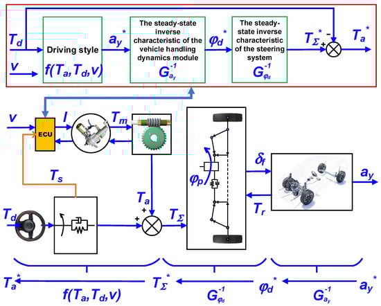
Figure 1.
The decomposition model of the EPS system.
Where: —the power-steering characteristic function represents the relationship between ( and (), this is the function that defines the driving style; —the inverse lateral acceleration-driver angle transfer function; and —the inverse steering torque—driver steering angle transfer function. The asterisk (*) on symbols represents the desired value of the quantity with the corresponding symbol; the other symbols of the system are shown in the Appendix A.
The “driving style calibration” module calculates the driver’s anticipated steering intensity, represented by lateral acceleration (is also the desired lateral acceleration to be achieved ), based on the torque steering () acting the steering wheel. This reflects the driver’s expected vehicle movement trend.
The “steady-state inverse characteristic of vehicle handling dynamics” is the inherent relationship between the lateral acceleration and the front wheel angle when the car reaches a steady state. Since the front wheel angle cannot be measured by on-board sensors, for the rack-and-pinion steering gearbox, the steering wheel angle (also the pinion angle) can be estimated by the motor speed, representing the steering Ackerman mechanism angle. The relationship between it and the front wheel angle is the angular steering gearbox ratio (). Therefore, the “steady-state inverse characteristic of vehicle handling dynamics” module () mentioned in this article is the inherent relationship between the lateral acceleration and steering wheel angle when the car reaches a steady state. This module calculates the steering wheel angle (which is also the desired steering wheel angle to be achieved ) through the expected lateral acceleration input (which is also the desired lateral acceleration to be achieved )—relationship .
The “steady-state inverse characteristic of the steering system” module illustrates the equivalent stiffness inherent relationship between the desired pinion angle and total torque required () (acting on the pinion) at a steady state. This module computes total torque () based on the steering wheel angle input () (relationship ).
Thus, the overall solution, as shown in Figure 1, can be summarized as follows: Based on the “driving-style calibration” module, determine the desired steering motion intensity to be achieved—represented by the desired lateral acceleration () under the influence of the input steering torque (). Next, the “steady-state inverse characteristic of vehicle handling dynamics” module calculates the desired steering wheel rotation angle () from input (). Next, the “steady-state inverse characteristic of the steering system” module calculates the required total torque () from input (). From () and (), calculate the required assist torque (). Based on the required (), the ECU sends the control current signal () to the assist motor, and the assist motor generates torque (). Through the worm gear transmission, it generates the actual assist torque (). From there, the actual total torque + = ) is transmitted to the pinion and makes the pinion achieve the desired rotation angle (also equal to ), then through the Ackermann mechanism, rotates the front wheel at an angle () from which the car achieves the steering motion intensity as the desired steering motion intensity, i.e., . The above modules will be implemented in the EPS controller. The proposed EPS system characteristic separation method has a good effect in separating the driver’s intention from the inherent dynamics of the vehicle and the steering system. This simplifies the calibration of the steering feel and facilitates the design of different driving styles on different types and models of vehicles.
3.2. Definition of the Inverse Relationship Between the Vehicle’s Lateral Acceleration and the Driver Angle
The inverse transfer function characteristics of the lateral acceleration and driver angle are determined through the vehicle motion dynamics and steering system dynamics.
Vehicle Motion Dynamics
The four-wheel (two-track) vehicle motion dynamics model is shown in Figure 2.
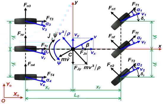
Figure 2.
Four-wheel vehicle motion dynamics model.
Applying D’Alembert’s principle, we have:
where: —total external force; —total inertial force; —total external moment; —total inertial moment; —acceleration; and —angular acceleration.
Thus, the system of equations of motion of the car projected onto the Cx, Cy axes and rotating around the Cz axis is:
where: —inertial force along axes Cx and Cy; ,—inertial force along axes Cx and Cy; and ,—centrifugal force along axes Cx and Cy. These forces are defined as follows:
Therefore, the differential equations describing the vehicle dynamics motion using the four-wheel model, are shown as follows:
where:
Equations (8) are written as follows:
In normal steady-state motion, the side-slip angle is usually very small. Therefore: = 1; . The dynamic Equation (10) is rewritten as follows:
For a front-axle driven vehicle (), the four-wheel vehicle motion model represented by the dynamic Equation (11) can be reduced to a two-wheel (bicycle) motion model with the following dynamic equation:
According to the kinetic relationship between the variables, we have:
From (13) and (14), we have:
When the wheel angle is small (; ). Therefore, the tire side slip angles at the two axles are defined as follows:
Considering the linearly deformed tire, the lateral tire forces are defined as follows [,,]:
Substitute (16)–(18) into Equation (12). The dynamic equation of the vehicle model is shown in Equation (19).
When the vehicle turns steadily (), and the longitudinal forces cancel (). Substitute () into the system of Equations (19) to obtain the following system of equations consisting of two equations:
From the structure of the steering system in Figure 3, the steering angle is determined as follows:
where:
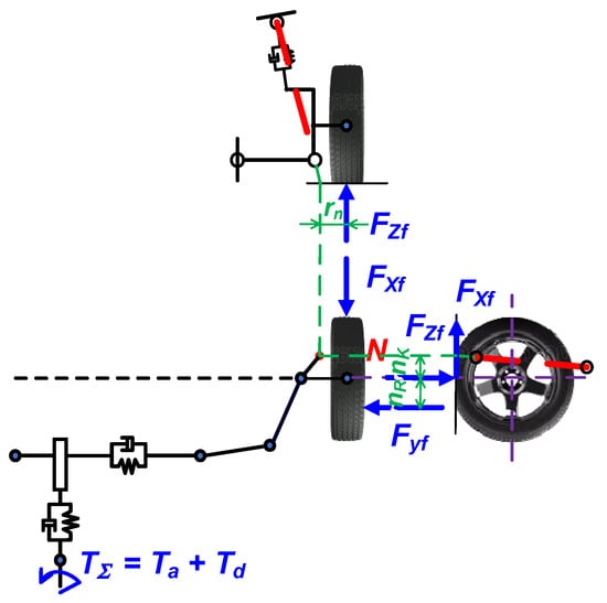
Figure 3.
EPS dynamics model.
Substitute (16) into Equation (21) to obtain the equation:
The following symbol is used:
Substitute (24), and (25) into Equations (20), and after simple transformation, the dynamic equation of the vehicle motion model is defined as follows:
Solving the above equations, the yaw rate angle transfer function of the vehicle body and the sideslip angle transfer function at the vehicle’s center of gravity are determined as follows:
where:
is the typical velocity (the velocity at which the yaw rate angle is most sensitive to the angle of the steering wheel rotation).
When the vehicle is turning steadily, the lateral acceleration is defined as:
Substitute (30) into Equations (27) to obtain the lateral acceleration transfer function , which is defined as follows:
The inverse lateral acceleration-driver angle transfer function is determined as follows:
3.3. Definition of the Inverse Relationship Between Steering Torque and Steering Driver Angle
The inverse steering torque–driver steering angle transfer function is determined:
4. Research on Building Ideal Steering Torque Characteristics
4.1. Constructing the Steering Torque and Lateral Acceleration Transfer Functions
From Equations (32) and (38), the transfer function of the steering torque and lateral acceleration is defined as follows:
The symbol is used:
The lateral acceleration is determined as:
From Equations (2) and (41), we have:
According to Equation (41), within the range of linear tire lateral deformation, the lateral acceleration response of the vehicle body according to the total moment acting on the steering colulm follows a linear relationship [,,].
4.2. Building Ideal Steering Torque Characteristics
The power-steering characteristics of the EPS system must meet the following essential requirements [,,]:
Low-operating torque: The system should provide minimal or no power assistance to ensure adequate road feel, stability, and reduced energy consumption.
Turning in place: Due to the largest resistance moment when the vehicle being turning in place, increased power output is necessary for sensitivity, but it should be limited to avoid excessive load and potential malfunctions.
Turning requirements: The assist torque from the motor must be lower than the corresponding steering resistance torque to prevent the phenomenon of “hand-beating”, which could lead to a loss of vehicle control.
Low speeds: At low speeds, high-resistance torque can diminish road feel. To ensure responsiveness, higher power output is needed, requiring appropriate gain settings.
Medium speeds: As vehicle speed increases, resistance torque and steering angle decrease while road feel’s requirements increase. The EPS system should reduce power assistance to balance sensitivity and road feel.
High speeds: At high speeds, the steering wheel angle changes minimally. Therefore, the EPS system should provide no assistance to maintain road feel and ensure stability and safety.
Gradual power adjustment: As vehicle speed increases during steering, power-assist gain adjustments should be gradual to prevent sudden jolts.
Power-assist limitations: There must be a threshold for power-assist limitations to prevent motor issues. Even if steering torque exceeds this threshold, the current should remain at the limit corresponding to the motor’s rated current.
Maximum steering torque: To ensure safe operation and comfortable driving without fatigue, the maximum steering torque for passenger car wheels is kept in the range (20 ÷ 50)N; for trucks or special vehicles, this range is (80 ÷ 100)N [,].
The power-assistance characteristic curve can be divided into three types as follows: (1) Linear type—first type: The power assistance increases linearly with the steering angle, ensuring a consistent and predictable response. However, this may lead to a less refined road feel, particularly at the transitions between the power-assistance dead zone and the changing zone. Furthermore, it does not adequately address the need for increased power-assistance torque when steering resistance suddenly rises. (2) Broken-line type—second type: The broken-line type features a segmented power-assistance approach, allowing for varied gains at different steering angles. However, this option can lead to a less smooth driving experience due to abrupt gain changes, potentially impacting the driver’s feel during transitions. (3) Nonlinear curve type third type: The nonlinear curve type offers a smooth, continuous relationship between steering torque and steering angle, allowing for a gradual increase in power assistance. This design enhances the driving experience with minimal impact on road feel, though its complexity can complicate adjustment and calibration.
Figure 4a,b show the are comparison of three types of power-assist characteristic curves. Figure 4a shows that when the maximum output power is the same, the first type is larger than the other two types, so this linear type is more sensitive. Figure 4b shows that when the steering feel is the same, the linear type has the smallest power-assist torque and poor performance after > . Based on the above requirements, the paper proposes a method for developing power-assistance characteristics corresponding to three different “driving styles” as follows:
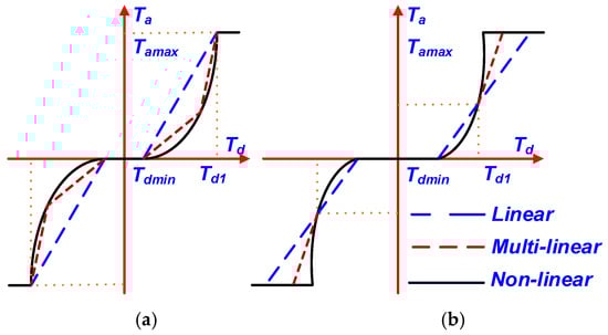
Figure 4.
Three types of power-assist characteristic curves: (a) The output power is the same; (b) the road feels the same.
4.2.1. Case 1: The Goal Is to Have a “Light and Comfortable Driving Feel”
In this case, the power-assistance torque is determined based on the following principles:
- (1)
- When , the power-assistance torque (the power-assistance motor is not activated);
- (2)
- When and , is calculated according to the linear characteristic, to take advantage of the high power of linear characteristics, ;
- (3)
- When and , is calculated according to the nonlinear characteristic to ensure the rapid increase of the power-assistance torque and high efficiency, ;
- (4)
- When , then , the power-assistance torque is maximized and does not increase further even if continues to grow.
- (5)
- When a vehicle is turning in place , there is high road resistance. Subsequently, the power-assistance torque must be large to ensure , from which the driver feels the need for a light and comfortable steering feel. When , depending on the speed, the power-assistance torque must reach its maximum value when the steering torque is in the range .
The power-assistance torque is determined in Equation (45):
where:
The sensitivity coefficient of the vehicle speed when the vehicle turns in place is defined as follows:
where: —the minimum steering torque required to activate the power-assistance system, it is chosen to ensure safety and steering feel when the road resistance torque is small; —the maximum steering torque that the driver needs to apply when the road resistance torque is maximum (); —actual steer torque according to the road resistance; —torque according to tire pressure standards []; and , —are determined through quadratic interpolation from experimental values.
4.2.2. Case 2: The Goal Is to Achieve a “Sporty Steering Feel”
In this case, the power-assistance torque is determined based on the following principles:
- (1)
- When the steering torque is small (takes at intersection ), the power-assistance torque , and the power-assistance motor is not activated);
- (2)
- When , the method of determining corresponds to Case 1. However, the level of assistance will be less than in Case 1 by an amount of .
- (3)
- When a vehicle is turning in place, the torque must be larger to ensure in the range of . In addition, when the driver applies a large enough steering force (about , the large value corresponding to high speed), the power-steering torque must reach its maximum value to ensure the convenience of steering operation when driving on difficult and complex terrain.
The power-assistance torque is determined in Equation (54):
where:
4.2.3. Case 3: “Multi-Level Driving Style”—The Goal Is to Achieve a Comfortable Driving Style at Low Speeds, a Sporting Style at Medium Speeds, and a Heavy, Safety Driving Feel at High Speeds
The power-assistance torque is determined in Equation (56):
In this case, the driver will have a light steering feeling at low speeds, a good road feeling at medium speeds, and a firm steering feeling at high speeds. Therefore, the power-steering torque is determined based on the following principles:
- (1)
- When the car is turning in place and when , the resistance from the road when turning is large. Therefore, must be large to ensure a light steering feel, maintaining in the range of .
- (2)
- When , the road resistance will decrease rapidly according to the car’s speed. So, to create a slightly heavier and sporty driving feel, acts according to Case 2.
- (3)
- When , the car speed range is the speed at which popular cars on the market that apply linear power-steering characteristic maps often force the power-steering system to be disconnected (i.e., there will be no more power steering) because at this time, the road-resistance torque is small, so to ensure the driving feeling, the power steering should be disconnected. In addition, in terms of the calculation algorithm, at this time, the coefficient has reached the minimum point, and if it continues to increase the car’s speed, then will increase. With the calculation method of the article, will continuously decrease. (Theoretically, the car’s speed can become very high ). Thus, with the above calculation method, the power steering is guaranteed to be very small and approaches 0 when the car has a speed of . From the above analysis, the article determines according to the following principles: when (where is the desired steering torque value to begin activating power assistance, it is selected ) to ensure good road feedback at high speeds. When , increases linearly with the steering torque, . However, the assist torque decreases rapidly with increasing vehicle speed because the coefficient decreases quickly with increasing vehicle speed (in this stage, ). When , then , the power-assistance torque is maximized and does not increase further even if continues to grow.
- (4)
- When and the road resistance is very small, only a small steering moment can create a large front wheel rotation angle, so it is necessary to limit this impact by providing power in the opposite direction to the steering direction, creating a heavy feeling of the steering wheel, with a fairly large steering torque still providing a small steering angle to ensure safety at very high speeds. Therefore, at very high speeds, to ensure safety when there are unwanted influences from the road or the driver on the steering wheel, when value is small , and then when , the motor will apply a torque opposite to the direction of . increases linearly but inversely with , (this stage ). When , and then , the power-assistance torque is maximized and does not increase further even if continues to grow.
Where: —adjustment speed for coefficient ; —limited assist torque at very high speeds.
5. Simulation Results Analysis
The simulation is conducted in three cases corresponding to the three driving style scenarios established above. The effective steering torque is . Trong đó is the largest steering torque acting on the steering wheel; we choose ; —tsimulation time; and -frequency of the steering torque. The selected values include: ; ; and .
The coefficients obtained through simulation experiments include: ; ; and .
5.1. Case 1: Light and Comfortable Driving Feel
The simulation results for “light and comfortable driving style” are shown in Figure 5.
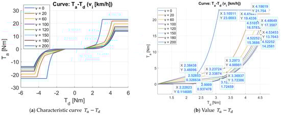
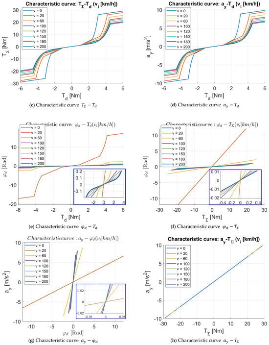
Figure 5.
Case 1-Light and comfortable driving style.
From the simulation results in Figure 5, we can see that: The requirements for constructing the power-assistance characteristics of Case 1 have been fulfilled; specifically:
- (1)
- From Figure 5a–c, when , then (the power-assistance motor is not activated); when , below the intersection point of the line and the curve , the assist torque follows the linear characteristic , and above the intersection point, the assist torque follows the non-linear characteristic . With , these intersection points correspond to and ;
- (2)
- Also following the aforementioned speeds, when , then and the assist torque reaches a maximum value , the assist torque does not increase further even if continues to grow.
- (3)
- From Figure 5a–d, when the driver applies an increasing steering torque , the assist torque and total torque also increase, resulting in an increased lateral acceleration of the vehicle, which means the rotational intensity increases.
- (4)
- From Figure 5d,e the characteristiscs of and correspond to different speeds. When applying the same value of steering torque, the lateral acceleration and the steering angle response are also different, and the level of lateral acceleration and the steering angle response decrease as the speed increases. In other words, to create the same value of lateral acceleration or the same value of the steering angle at higher speeds, the steering torque needs to be applied more. This will make the driver feel the steering wheel is heavier at high speeds, thereby increasing safety when driving at high speeds.
- (5)
- Similarly, Figure 5f shows the characteristics between the steering angle and the total torque applied to the pinion , and Figure 5g shows the characteristics between the steering angle and lateral acceleration . It can be seen that at the same speed, the relationship between is linear, which provides the driver a consistent steering feel at the same speed. As the speed increases, the slope of the a–b characteristic decreases quite rapidly, which means that to create the same steering angle at higher speeds, a larger steering torque is required, thus creating a feeling of firmness in the steering wheel at high speeds to improve control safety. On the contrary, as the speed increases, the slope of the characteristic increases rapidly, which means that at higher speeds, the lateral acceleration is more sensitive to the steering angle, so creating a heavy steering feel to reduce the steering angle at high speeds is necessary.
- (6)
- From Figure 5h, the characteristic of is the linear relationship, independent of vehicle speed. This ensures a consistent steering feel.
- (7)
- Figure 5i,j are the response of the power-steering torque and total torque when steering sinusoidally. The results also show that the established principles are implemented.
Thus, with the above power-assist characteristics, the requirements of the power-assist characteristics set forth in Section 4.2 are all achieved. In addition, the power-assist motor is activated early with this power-assist characteristic. Corresponding to different speeds, the power-assistance torque has reached the maximum value, while the steering torque is maintained in the range of . Therefore, the driver will have a “light and comfortable driving feeling”.
5.2. Case 2: Sporty Steering Feel
The simulation results for a “sporty driving style” are shown in Figure 6.
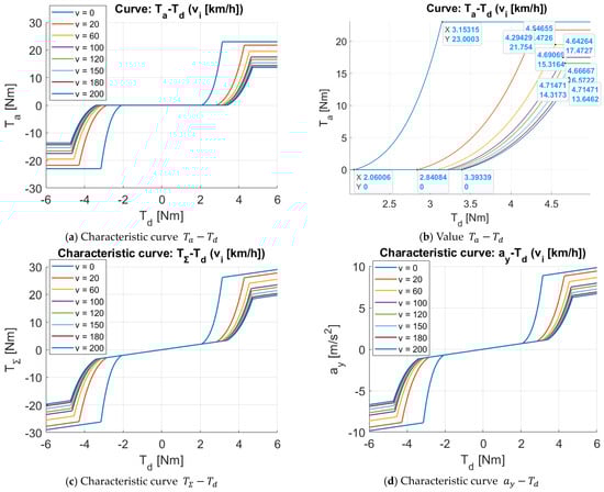
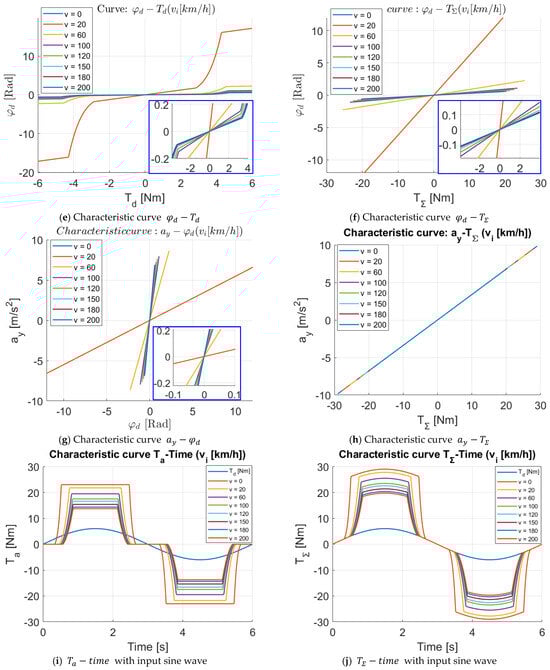
Figure 6.
Case 2-Sporty steering style.
From the simulation results in Figure 6, it can be seen that: The requirements for constructing the power-assistance characteristics of Case 2 have been fulfilled, specifically:
- (1)
- From Figure 6a,b, the power-steering motor is only activated when , and the value gradually increases as the vehicle speed increases. When activating the power steering, the assist torque increases nonlinearly according to , but the characteristic curve’s slope is lower than the increase of “Case 1”.
- (2)
- Corresponding to different speeds, the power-steering torque when . The values at the transition points of the characteristic curve are shown in Figure 6b.
- (3)
- Other results are similar to Case 1.
Thus, with this power-steering characteristic curve, the power-steering torque is activated late, and when activated, the power-steering torque does not increase quickly. At the same time, the assist torque reaches its maximum when the steering torque reaches a relatively large value . Therefore, the driver will have a more “firm” driving feeling, or, in other words, a more “sporty driving style”.
5.3. Case 3: Multi-Level Driving Feel Style (Comfortable Driving Style at Low Speed, Sport Style at Medium Speed, and Heavy, Safety Driving Feel at High Speed)
The simulation results for the “multi-level driving feel style” are shown in Figure 7.
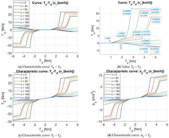
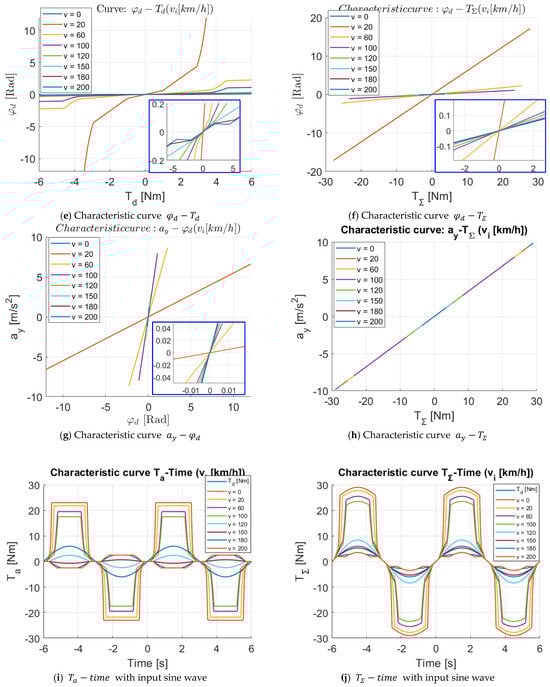
Figure 7.
Case 3-Multi-level driving feel style.
From the simulation results in Figure 7, it can be seen that:
The requirements for constructing the power-assistance characteristics of Case 3 have been fulfilled, specifically:
- (1)
- When , the characteristic curve is constructed, as in Case 1;
- (2)
- When , the assist torque acts according to Case 2;
- (3)
- When , while , then , and when , then increases according to the linear characteristic to reduce the torque support compared to the nonlinear characteristic;
- (4)
- When , when , then . When , then and increases in the opposite direction to until , which will not continue to increase even though continues to increase. (However, in actual vehicle operation, the case of steering with large torque at high speeds rarely happens);
- (5)
- The values at the transition points of the characteristic curve are shown in Figure 7b.
With this characteristic, the driver will have a “comfortable driving feel at low speed, sport feel at medium speed, and heavy, safety feel at high speed”.
6. Conclusions
This paper aims to solve the problem of improving the steering feel and performance of the EPS system to meet the driver’s expectations when the steering force reaches the desired steering motion intensity. The paper proposes a method to construct the ideal EPS characteristics by analyzing the inverse dynamic characteristics, separating the driver’s control intention from the inherent dynamics of the vehicle and the steering system, thereby determining the power-steering characteristics according to the desired driving styles. By establishing the ideal relationship between the steering torque and the steering motion intensity in accordance with Stevens’s psychological law, a theoretical basis for the design and adjustment of the steering feel is provided. The non-linear relationship between the power-steering torque and the vehicle speed and the steering torque in the EPS system is analyzed into three functional modules: the driving style module; the inverse dynamic characteristics module of the vehicle’s motion; and the inverse dynamic characteristics module of the steering system. The simulation results show that the calculations of the driver’s impact force, the power-steering torque support level, and the maximum power-steering torque value are all consistent. The results of the paper are also an important basis for research on control integration in active driving cars [] and automatic cars at levels 2 to 3 []. This is also a research direction of the authors.
Some challenges of the proposed method that need further development: the assumption of a fixed power exponent in the relationship between steering torque and lateral acceleration. David J. Weiss argued that Stevens’ power law is not universally applicable due to its dependence on measurement assumptions, variations in sensory modality exponent values, and contextual influences. In this case, the exponent may not be constant across different driving conditions, vehicle types, or driver preferences, making the model potentially inaccurate for diverse real-world scenarios. Additionally, while the method incorporates speed influence through parameters and , it does not fully address variations in road conditions, vehicle load, and driver perception biases. If empirical studies demonstrate significant variations under different driving scenarios, Weiss’ critique that no single function universally defines perception becomes more relevant. Future research should refine the model by introducing a speed-zone-divided power-steering characteristic map, integrating dynamic load factors and road adhesion variations to enhance real-world applicability. In the future, some experiments to demonstrate the effectiveness of the proposed method are interesting topics.
Author Contributions
Conceptualization, H.Q.N. and V.T.V.; methodology, H.Q.N. and O.S.; software, H.Q.N.; validation, H.Q.N., V.T.V., and O.S.; formal analysis, H.Q.N.; investigation, V.T.V.; resources, H.Q.N.; data curation, H.Q.N.; writing—original draft preparation, H.Q.N.; writing—review and editing, V.T.V. and O.S.; visualization, V.T.V.; supervision, O.S.; project administration, H.Q.N.; funding acquisition, H.Q.N. All authors have read and agreed to the published version of the manuscript.
Funding
This research received no external funding.
Data Availability Statement
In this paper, the research results are novel and not previously published. The approach, research methods, research results and analysis, and evaluation are all directly conducted by the authors.
Conflicts of Interest
The authors declare no conflict of interest.
Abbreviations
The following abbreviations are used in this manuscript:
| EPS | Electric Power Steering |
| CNS | Central Nervous System |
Appendix A

Table A1.
Symbol of the EPS system.
Table A1.
Symbol of the EPS system.
| Symbol | Description | Unit |
|---|---|---|
| Driver torque | ||
| Assist torque | ||
| Total torque | ||
| Road reaction torque | ||
| The torque when the power steering is activated | ||
| Lateral force | ||
| Longitudinal force at front axle | ||
| Longitudinal force at rear axle | ||
| Lateral force at front axle | ||
| Vertical force at front axle | ||
| Vehicle sideslip angle | ||
| Vehicle yaw angle | ||
| Steer angle | ||
| Front tire sideslip angle | ||
| Rear tire sideslip angle | ||
| Kingpin angle | ||
| Camber angle | ||
| , | Vehicle speed sensitivity coefficient | |
| Vehicle speed sensitivity coefficient in parking | ||
| Adhesion coefficient (friction) | ||
| Steering system efficiency | ||
| Tire pneumatic trail | ||
| Kingpin forward indicator | ||
| Total offset | ||
| Turning radius | ||
| Wheelbase | ||
| Ox-axis distance of axle from the mass center | ||
| Oy-axis distance of axle from the mass center | ||
| Ox-axis distance of front axle from the mass center | ||
| Oy-axis distance of rear axle from the mass center | ||
| Wheel radius | ||
| Tyre lateral stiffness coefficient | ||
| Front tire sideslip coefficient | ||
| Rear tire sideslip coefficient | ||
| Steering system stiffness | ||
| Vehicle speed | ||
| Vehicle characteristic speed | ||
| ; | Front and rear wheel Longitudinal speeds | |
| Lateral acceleration | ||
| Vehicle mass | ||
| Vehicle moment of inertia | ||
| Tyre standard pressure | ||
| Steering gear ratio |
References
- Hung, Y.C.; Lin, F.J.; Hwang, J.C.; Chang, J.K.; Ruan, K.C. Wavelet fuzzy neural network with asymmetric membership function controller for electric power steering system via improved differential evolution. IEEE Trans. Power Electron. 2015, 30, 2350–2362. [Google Scholar] [CrossRef]
- Wilhelm, F.; Tamura, T.; Fuchs, R.; Müllhaupt, P. Friction compensation control for power steering. IEEE Trans. Control Syst. Technol. 2016, 24, 1354–1367. [Google Scholar] [CrossRef]
- Kim, W.; Seop Son, Y.; Chung, C.C. Torque overlay-based robust steering wheel angle control of electrical power steering for a lane-keeping system of automated vehicles. IEEE Trans. Veh. Technol. 2016, 65, 4379–4392. [Google Scholar] [CrossRef]
- Ruba, M.; Nemes, R.; Piglesan, F.P.; Martis, C. Complete electric power steering system real-time model in the loop simulator. ELEKTRO, 2018; in print. [Google Scholar] [CrossRef]
- Badawy, A.; Zuraski, J.; Bolourchi, F.; Chandy, A. Modeling and Analysis of an Electric Power Steering System; SAE Technical paper 1999-01-0399; SAE: Warrendale, PA, USA, 1999. [Google Scholar] [CrossRef]
- Van Tan, V.; Sename, O.; Gaspar, P.; Do, T.T. Active Anti-Roll Bar Control Design for Heavy Vehicles; Springer: Berlin, Germany, 2024. [Google Scholar] [CrossRef]
- Choi, J.H.; Nam, K.; Oh, S. Steering feel improvement by mathematical modeling of the Electric Power Steering system. Mechatronics 2021, 78, 102629. [Google Scholar] [CrossRef]
- Irmer, M.; Henrichfreise, H. Design of a robust LQG compensator for an electric power steering. IFAC-papersOnLine 2020, 53, 6624–6630. [Google Scholar] [CrossRef]
- Morita, Y.; Yokoi, A.; Iwasaki, M.; Ukai, H.; Matsui, N.; Ito, N.; Uryu, N.; Mukai, Y. Controller Design Method for Electric Power Steering System with Variable Gear Transmission System using Decoupling Control. In Proceedings of the 35th Annual Conference of IEEE Industrial Electronics, Porto, Portugal, 3–5 November 2009. [Google Scholar] [CrossRef]
- Yamamoto, K.; Sename, O.; Koenig, D.; Moulaire, P. Design and experimentation of an LPV extended state feedback control on Electric Power Steering systems. Control Eng. Pract. 2019, 90, 123–132. [Google Scholar] [CrossRef]
- Du, P.-P.; Su, H.; Tang, G.-Y. Active Return-to-Center Control Based on Torque and Angle Sensors for Electric Power Steering Systems. Sensors 2018, 18, 855. [Google Scholar] [CrossRef]
- Guan, X.; Zhang, Y.-N.; Duan, C.-G.; Yong, W.-L.; Lu, P.-P. Study on decomposition and calculation method of EPS assist characteristic curve. Proc. Inst. Mech. Eng. Part D J. Automob. Eng. 2021, 235, 2166–2175. [Google Scholar] [CrossRef]
- Zhang, N.; Cai, T.; Han, X. Electric power steering system controller design using induction machine. Arch. Electr. Eng. 2019, 68, 279–293. [Google Scholar] [CrossRef]
- Xue, M.; Xu, G.; Feng, J.; Meizhou, C.; Xu, H. Control strategy of automotive electric power steering system based on generalized internal model control. J. Algorithms Comput. Technol. 2020, 14, 1–9. [Google Scholar] [CrossRef]
- Zang, H.; Chen, S. Electric Power Steering Simulation Analyze Based on Fuzzy PID Current Tracking Control. J. Comput. Inf. Syst. 2011, 7, 119–126. [Google Scholar]
- Li, Y.; Yang, Z.; Zhai, D.; He, J.; Fan, J. Study on Control Strategy of Electric Power Steering for Commercial Vehicle Based on Multi-Map. World Electr. Veh. J. 2023, 14, 33. [Google Scholar] [CrossRef]
- Zhao, W.; Lin, Y.; Wei, J.; Shi, G. Control strategy of a novel electric power steering system integrated with active front steering function. Sci. China Technol. Sci. 2011, 54, 1515–1520. [Google Scholar] [CrossRef]
- Shi, S.; Chen, G. Electric-Power-Steering system Vehicle Control Stability and Return Strategies Based on Predictive Control. J. Eng. Sci. Technol. Rev. 2022, 15, 146–153. [Google Scholar] [CrossRef]
- Yamamoto, K.-i.; Nishimura, H. Control System Design of Electric Power Steering for a Full Vehicle Model with Active Stabilizer. J. Syst. Des. Dyn. 2011, 5, 789–804. [Google Scholar] [CrossRef][Green Version]
- Ma, X.; Guo, Y.; Chen, L. Active disturbance rejection control for electric power steering system with assist motor variable mode. J. Franklin Inst. 2018, 355, 1139–1155. [Google Scholar] [CrossRef]
- Lee, D.; Kim, K.-S.; Kim, S. Controller design of an electric power steering system. IEEE Trans. Control. Syst. Technol. 2018, 26, 748–755. [Google Scholar] [CrossRef]
- Woo, S.; Heo, C.; Jeong, M.-O.; Lee, J.-M. Integral Analysis of a Vehicle and Electric Power Steering Logic for Improving Steering Feel Performance. Appl. Sci. 2023, 13, 11598. [Google Scholar] [CrossRef]
- Saifia, D.; Chadli, M.; Karimi, H.R.; Labiod, S. Fuzzy control for Electric Power Steering System with assist motor current input constraints. J. Frankl. Inst. 2015, 352, 562–576. [Google Scholar] [CrossRef]
- Zheng, Z.; Wei, J. Research on active disturbance rejection control strategy of electric power steering system under extreme working conditions. Meas. Control 2024, 57, 90–100. [Google Scholar] [CrossRef]
- Zhang, H.; Zhang, Y.; Liu, J.; Ren, J.; Gao, Y. Modeling and characteristic curves of electric power steering system. In Proceedings of the 2009 International Conference on Power Electronics and Drive Systems (PEDS), Taipei, Taiwan, 2–5 November 2009. [Google Scholar] [CrossRef]
- Li, S.; Sheng, R.; Cui, G.; Zheng, S.; Yu, Z.; Lu, X. Design of Assistance Characteristics Curve for Electric Power Steering System. Atlantis Press 2017, 87, 129–133. [Google Scholar] [CrossRef][Green Version]
- Du, S.; Yao, L. Design of Assisted Characteristic Curve for Electric Power Steering System Based on Load Variation. Int. J. Res. Eng. Sci. (IJRES) 2016, 4, 53–58. Available online: https://www.ijres.org/v4-i10.html (accessed on 25 December 2024).
- Zhao, X.-P.; Li, X.; Chen, J.; Men, J.-L. Parametric design and application of steering characteristic curve in control for electric power steering. Mechatronics 2009, 19, 905–911. [Google Scholar] [CrossRef]
- Ciarla, V.; Cahouet, V.; de Wit, C.C.; Quaine, F. Genesis of booster curves in Electric Power Assistance Steering systems. In Proceedings of the 2012 15th International IEEE Conference on Intelligent Transportation Systems, Anchorage, AK, USA, 16–19 September 2012; pp. 1345–1350. [Google Scholar] [CrossRef]
- Hosman, R.J.A.W.; Cardullo, F.M.; Bos, J.E. Visual-Vestibular interaction in motion perception. In Proceedings of the AIAA Modeling and Simulation Technologies Conference, Portland, OR, USA, 8–11 August 2011. [Google Scholar] [CrossRef]
- Shinar, D.; Mcdowell, E.D.; Rockwel, T.H. Eye Movements in Curve Negotiation. Human Factors 1977, 19, 63–71. [Google Scholar] [CrossRef]
- Donald, A. Gordon. Static and dynamic visul fields in human space perception. J. Opt. Soc. Am. 1965, 55, 1296–1303. Available online: https://opg.optica.org/josa/abstract.cfm?URI=josa-55-10-1296 (accessed on 21 December 2024).
- Lone, M.; Cooke, A. Review of Pilot Modelling Techniques. In Proceedings of the 48th AIAA Aerospace Sciences Meeting Including the New Horizons Forum and Aerospace Exposition, Orlando, FL, USA, 4–7 January 2010. [Google Scholar] [CrossRef]
- Young, L.R.; Meiry, J.L. A revised dynamic otolith model. Aerosp. Med. 1968, 39, 606–608. [Google Scholar] [PubMed]
- Fechner, G.T. Elemente der Psychophysik; Breitkopf u. Härtel: Leipzig, Germany, 1860. [Google Scholar]
- Newberry, A.C.; Griffin, M.J.; Dowson, M. Driver Perception of Steering Feel. Proc. Inst. Mech. Eng. Part D-J. Automob. Eng. 2007, 221, 405–415. [Google Scholar] [CrossRef]
- Stevens, S.S. On the Psychophysical Law. Psychol. Rev. 1957, 64, 153–181. [Google Scholar] [CrossRef]
- Guo, X. Experimental Psychology, 2nd ed.; People’s Education Press: Beijing, China, 2019. [Google Scholar]
- Yu, Z. Automobile Theory, 6th ed.; Machinery Industry Press: Beijing, China, 2018; p. 197. [Google Scholar]
- Liu, Z. Automobile Science; Higher Education Press: Beijing, China, 2012; p. 629. [Google Scholar]
- Mitschke, M. Henning Wallentowitz. Dynamik der Kraftfahrzeuge; Springer Vieweg Wiesbaden: Berlin/Heidelberg, Germany, 2014; ISBN 978-3-658-05067-2. [Google Scholar] [CrossRef]
- Weiss, D.J. The impossible dream of Fechner and Stevens. Perception 1981, 10, 431–434. [Google Scholar] [CrossRef]
- Guo, K. Automobile Handling Dynamics; Jilin Science and Technology Press: Changchun, China, 1991. [Google Scholar]
- Shi, G.; Shen, R.; Lin, Y. Modeling and simulation technology of electric power steering system. J. Jilin Univ. 2007, 37, 31–36. [Google Scholar]
- GB/T 6323-2014; General Administration of Quality Supervision, Inspection and Quarantine of the People’s Republic of China, Administration of Standardization of the People’s Republic of China. China Standards Press: Beijing, China, 2014.
- Liang, J.; Lu, Y.; Yin, G.; Fang, Z.; Zhuang, W.; Ren, Y.; Xu, L.; Li, Y. A Distributed Integrated Control Architecture of AFS and DYC Based on MAS for Distributed Drive Electric Vehicles. IEEE Trans. Veh. Technol. 2021, 70, 5565–5577. [Google Scholar] [CrossRef]
- Wiseman, Y. Autonomous Vehicles. In Encyclopedia of Information Science and Technology, 5th ed.; IGI Global: Hershey, PA, USA, 2020; pp. 1–11. [Google Scholar] [CrossRef]
Disclaimer/Publisher’s Note: The statements, opinions and data contained in all publications are solely those of the individual author(s) and contributor(s) and not of MDPI and/or the editor(s). MDPI and/or the editor(s) disclaim responsibility for any injury to people or property resulting from any ideas, methods, instructions or products referred to in the content. |
© 2025 by the authors. Licensee MDPI, Basel, Switzerland. This article is an open access article distributed under the terms and conditions of the Creative Commons Attribution (CC BY) license (https://creativecommons.org/licenses/by/4.0/).