FMV-YOLO: A Steel Surface Defect Detection Algorithm for Real-World Scenarios

Abstract

Surface defects during steel production can severely impact product quality and safety, making defect detection crucial. To improve the precision and performance of conventional approaches, we introduce FMV-YOLO, a model for detecting steel surface defects, built upon YOLOv11n. First, we substitute the C2PSA attention module in the backbone network with an Adaptive Fine-Grained Channel Attention (FCA) module, which improves defect type identification while reducing the parameter count. Next, we incorporate a new Multi-Scale Attention Fusion module (MSAF) to strengthen feature representation and refine the loss function using Normalized Wasserstein Distance (NWD) loss, thereby improving the localization accuracy of small defects. Finally, we integrate the VoV-GSCSP module within the neck network to achieve lightweighting, facilitating real-world deployment. Extensive experiments on the GC10DET and NEU-DET datasets demonstrate that the model effectively balances detection accuracy, parameter count, and computational load. With 2.6M parameters and 5.7G FLOPs, the model attains an mAP@0.5 of 73.4% on GC10DET and 80.2% on NEU-DET. Additionally, the method achieves 99% detection accuracy on a self-constructed industrial dataset, proving its effectiveness in industrial defect detection.

1. Introduction

Steel, as a fundamental material, is essential for fostering socio-economic growth and advancing technology. Without steel as a raw material, modern infrastructure would be impossible. Steel types are diverse, including carbon steel (e.g., low-, medium-, and high-carbon steel) [1], tool steel, stainless steel, alloy steel, and specialty steel [2]. Each type, with its unique chemical composition and physical properties, is suited for different industrial applications. For instance, stainless steel [3] is widely used in food processing and medical devices due to its corrosion resistance, while high-carbon steel is often employed in manufacturing tools and springs due to its high hardness. However, during steel production, surface defects encompassing inclusions, creases, and spots inevitably occur due to complex processes and variable environmental conditions [4]. These defects directly impact the appearance, mechanical properties, and performance of steel [5]. Efficient defect detection technologies enable real-time identification and localization of these defects during production, improving product reliability, reducing costs, minimizing resource waste, and promoting sustainable development [6]. Therefore, developing an effective steel surface defect detection system tailored to real industrial scenarios is crucial to maintaining product standards and preventing defective items from entering the market.

Conventional approaches for detecting steel surface defects predominantly depend on manual examination [7] and basic equipment, such as high-resolution cameras, microscopes, ultrasonic testing, and X-ray inspection [8]. While these methods can identify surface and internal defects to some extent, they are often limited by high costs, operational complexity, and slow detection speeds, rendering them inadequate for extensive industrial manufacturing. As deep learning technology has progressed, researchers have increasingly utilized deep learning algorithms for defect detection tasks. However, difficulties persist in real industrial scenarios. First, the detection of multiple defect types is complex owing to the diversity of steel surface defects, where variations within the same class can be significant, while differences between classes may be minimal [9], leading to frequent misdetections. To address this, we introduce the Adaptive Fine-Grained Channel Attention (FCA) mechanism and the Multi-Scale Attention Fusion (MSAF) module to improve detection accuracy. Second, detecting small-target defects [10] is challenging. Small targets, such as those with pixel sizes below 32 × 32 in the COCO dataset or occupying less than 10% of the image, are common on steel surfaces (e.g., water spots, oil spots). To tackle this, we incorporate the Normalized Wasserstein Distance (NWD) loss function, weighted with the original loss function, to improve the model’s localization capability for small defects. Finally, real-time detection is crucial in industrial environments with constrained computational resources. To meet this demand, we introduce the VoV-GSCSP module in the neck network to achieve lightweight, real-time defect detection.

In conclusion, the key contributions of this paper are outlined below:

• We constructed a custom steel surface defect dataset for real industrial scenarios, which will greatly assist enterprises in achieving steel defect detection.
• To improve the integration of global and local information, the Adaptive Fine-Grained Channel Attention (FCA) mechanism was introduced to replace the C2PSA attention module. This modification enables more effective weight allocation and facilitates the extraction of highly informative features.
• To further enhance the model’s effectiveness in detecting objects across different scales, we introduced a novel Multi-Scale Attention Fusion (MSAF) module. Additionally, by optimizing the bounding box regression using a weighted combination of the Normalized Wasserstein Distance (NWD) and CIoU, it effectively compensates for the shortcomings of IoU loss in small object detection, resulting in smoother predictions for small targets by the model.
• To address the need for detection speed from enterprises, we introduced VOVGSCSP in the neck network for lightweight processing from the perspective of model complexity.

Extensive experiments conducted on the GC10DET and NEU-DET datasets demonstrate that FMV-YOLO achieves an optimal balance among detection accuracy, parameter efficiency, and computational load. Specifically, the proposed model attains an mAP@0.5 of 73.4% on GC10DET and 80.2% on NEU-DET, while maintaining a lightweight architecture with only 2.6M parameters and a computational cost of 5.7G FLOPs, making it well suited for real-time industrial deployment. Furthermore, on a self-constructed industrial dataset, the model achieves an impressive 99% detection accuracy, demonstrating its effectiveness in practical defect detection applications.

The subsequent sections of this paper are organized as follows: In Section 2, the differences between related work and the work presented in this paper are compared. Section 3 details the dataset and the architecture and principles of the proposed FMV-YOLO model. Section 4 discusses the experimental results and comparative analyses. Finally, Section 5 offers the conclusion of this paper.

2. Related Works

With the advancement of artificial intelligence technology, computer vision has been increasingly applied in industrial scenarios. Currently, defect detection methods are mainly divided into two categories: Conventional methods, including SVM and decision trees, depend on manually designed feature extraction, which often leads to constrained accuracy and real-time capabilities. For example, the Multi-Hyperplane Twin Support Vector Machine (MHTSVM) proposed in [11] performs well in steel surface defect recognition but is still constrained by the inherent limitations of traditional methods. The other category is deep learning algorithms, which are primarily categorized into two-stage (e.g., Faster-RCNN [12]) and one-stage (e.g., SSD, YOLO series) algorithms. One-stage algorithms, with their simpler structures and faster detection speeds, such as SSD [13] based on the VGG16 framework, employ multi-scale feature prediction to enhance detection speed and accuracy. In recent years, the YOLO series algorithms [14] have attracted considerable attention owing to their balance between accuracy and speed, becoming widely used in steel surface defect detection.

Building on these technologies, researchers have made notable progress in defect detection. In reference [15], an enhanced Non-Maximum Suppression (NMS) method was introduced to minimize redundant bounding boxes and enhance detection performance. Reference [16] combined the Feature Pyramid Network (FPN) and the Region Proposal Network (RPN) to propose a Swin Transformer-based defect detection method. Reference [17] introduced the Initial Dynamic Texture Enhancement Module (IDTEM) to enhance the detection accuracy of defects with low contrast. Reference [18] integrated segmentation and object detection models (e.g., U-Net, FCN-8, FPN, and YOLOv4) and developed a two-stage detection architecture to optimize small defect detection. Reference [19] proposed a YOLOv5-based multi-scale exploration module to enhance detection performance. Reference [20] improved YOLOv8 by introducing the Adaptive Feature Extraction (AFE) module, Triplet Attention module, and GSConv, strengthening feature extraction and small defect detection capabilities. Reference [21] designed the C2f-DS module combined with the Large Selective Kernel (LSK) attention mechanism to address the low accuracy and efficiency of traditional methods. Reference [22] enhanced the YOLOv9 model to address the loss of shallow information and inadequate feature fusion resulting from network deepening.

Although the aforementioned methods have achieved significant progress, there remains significant potential for enhancement and refinement in steel surface defect detection. Many existing studies primarily focus on enhancing individual modules, while few have achieved a well-balanced trade-off among detection accuracy, computational complexity, and model lightweighting—a crucial factor for real-time industrial defect detection and efficient deployment.To better evaluate the robustness and generalization capability of the proposed model while considering the latest advancements in current detection technologies, this paper conducts a thorough assessment of the performance of YOLOv5, YOLOv8, YOLOv10, and the latest YOLOv11 methods in the task of steel surface defect detection. It concludes that YOLOv11 offers the most balanced performance in terms of parameter count, computational load, and detection accuracy. Therefore, this paper employs YOLOv11 for our detection tasks and further refines the YOLOv11 network to develop a superior algorithm. Additionally, we have independently constructed a dataset of steel surface defects from real industrial environments to validate the performance of the model we have proposed.

3. Methods

In this section, we provide a comprehensive explanation of the proposed FMV-YOLO model, detailing each module in the network architecture and clarifying their respective functions. First, we present an overview of the entire model, followed by an introduction to YOLOv11, which serves as the baseline for our improvements. We then provide a detailed description of the key components, including the Adaptive Fine-Grained Channel Attention (FCA) module, the Multi-Scale Attention Fusion (MSAF) module, the Normalized Wasserstein Distance (NWD) loss function, and the VoV-GSCSP module. These enhancements collectively contribute to improved feature extraction, enhanced small defect localization, and an optimized lightweight network design, making the model more suitable for real-world industrial defect detection.

3.1. Overview

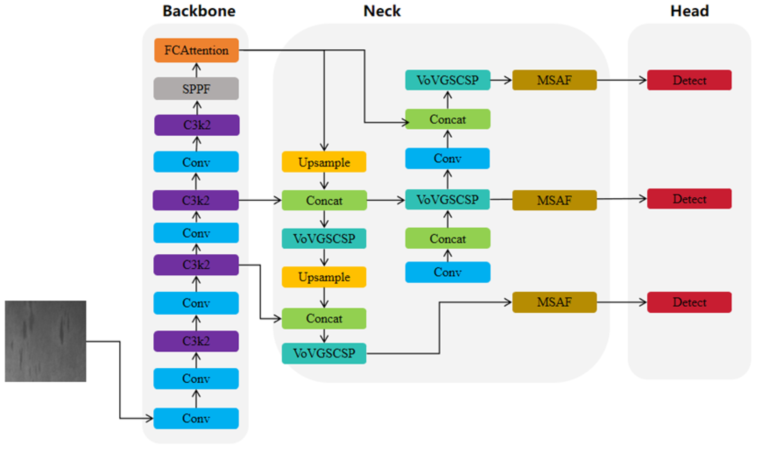
The framework of the FMV-YOLO model, improved based on YOLOv11, is illustrated in Figure 1. Firstly, the C2PSA in the backbone network is replaced with the Adaptive Fine-Grained Channel Attention (FCA) mechanism to more effectively fuse global and local information, optimize channel feature weights, improve detection accuracy, and reduce computational costs. Secondly, a Multi-Scale Attention Fusion module (MSAF) is introduced before the detection head to accommodate variations in defect sizes. Additionally, the Normalized Wasserstein Distance (NWD) is incorporated on top of CIoU, enabling the model to focus more on tiny defects and improving target localization capabilities. Finally, to meet practical application requirements, the C3k2 module in the neck network is replaced with VoV-GSCSP to achieve a balance between detection accuracy and speed.

FCA, MSAF, and NWD synergistically contribute to the detection of steel surface defects through multi-level interactions. Firstly, FCA optimizes channel attention by constructing global and local information, making the input features to MSAF more significant. MSAF further leverages attention mechanisms at different scales to explore relationships between features, achieving comprehensive fusion of multi-scale features. Secondly, MSAF enhances the detailed information of small targets, improving the clarity of small-target feature representation, thereby optimizing the stability of NWD in bounding box adjustment. NWD relies on precise feature representation, so after MSAF provides higher-quality small-target features, NWD can more accurately regress the bounding boxes of small targets. Furthermore, NWD promotes the learning of FCA and MSAF during the loss optimization process. Since NWD focuses on the robustness of small-target detection, its supervision signals can further encourage the network to pay attention to small-target features, thereby enhancing the overall learning effectiveness of FCA and MSAF and making them more suitable for extracting and characterizing features in small-target detection tasks.

3.2. YOLOv11

YOLOv11 [23], introduced by Ultralytics in 2024, is the latest algorithm in the YOLO series, representing a significant leap forward in real-time object detection technology. Based on the depth and width of the model, YOLOv11 can be divided into multiple versions, including YOLOv11n, YOLOv11s, YOLOv11m, YOLOv11l, and YOLOv11x. As the network depth and width parameters increase, the model size grows, generally improving accuracy, but the detection speed may decrease. 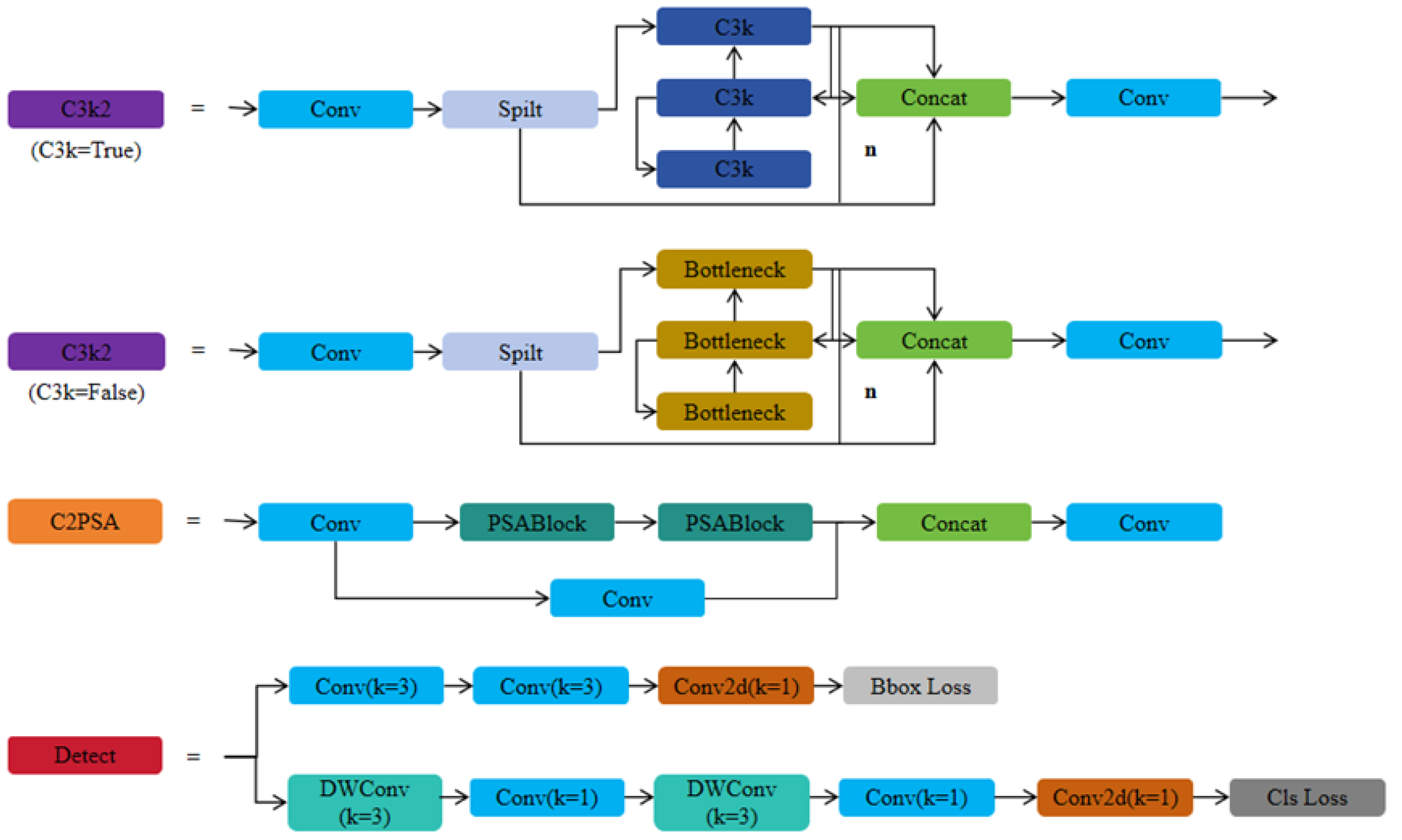Compared to the previous generation YOLOv8 [24] by Ultralytics, YOLOv11 does not have major changes. The changes involve replacing C2f with C3k2, adding a layer similar to an attention mechanism, C2PSA, after the SPPF, and replacing two DWConv layers inside the detection head. The loss function continues to use CIoU as the bounding box regression loss. The network architecture and module structure diagrams are shown in Figure 2 and Figure 3. Considering the real-time requirements for steel surface defect detection, this study selects YOLOv11n as the baseline model.

3.3. Adaptive Fine-Grained Channel Attention

Attention mechanisms are indispensable tools in deep learning, as they can dynamically select important features, enabling models to focus more on the most relevant parts of a task, thereby improving performance. In recent years, channel attention mechanisms, like the Squeeze-and-Excitation (SE) mechanism, have found extensive use in a variety of visual detection tasks. Although the SE mechanism [25] effectively extracts global features through fully connected layers, it lacks sufficient utilization of local information. Based on this, we introduce an Adaptive Fine-Grained Channel Attention (FCA) mechanism [26] to dynamically integrate such information.

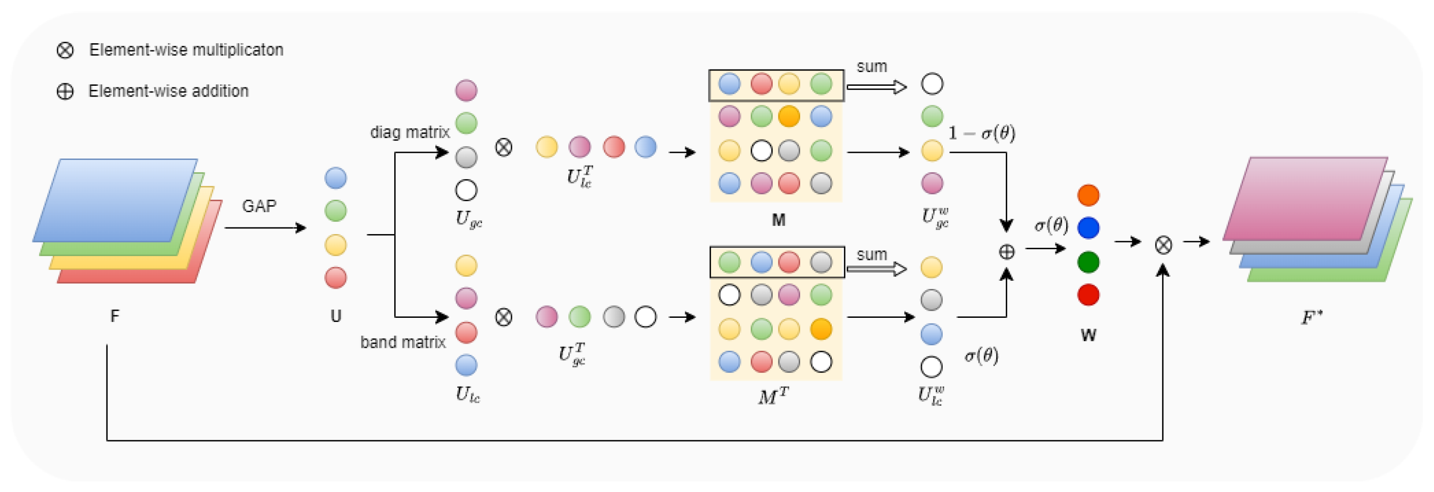
The framework of this mechanism is shown in Figure 4. Given a feature map $F\in R^{C\times H\times W}$, its dimensions are first reduced to $C\times 1\times 1$ using global average pooling. Subsequently, a band matrix B and a diagonal matrix D are introduced to capture local and global information among channels, respectively, where $B=[b_1,b_2,b_3,\dots ,b_i]$ and $D=[d_1,d_2,d_3,\dots ,d_i]$. The detailed calculations are as follows:

$$U_{lc}=\sum _{i=1}^{k}U•b_i$$

(1)

$$U_{gc}=\sum _{i=1}^{c}U•d_i$$

(2)

Here, U represents the channel descriptor obtained from the first step, $U_{lc}$ denotes local information, $U_{gc}$ denotes global information, k is the number of adjacent channels, and c is the total number of channels.

After obtaining the local information $U_{lc}$ and global information $U_{gc}$, their interaction is further enhanced through cross-correlation operations, resulting in the correlation matrix M:

$$M=U_{gc}•U_{lc}^T$$

(3)

Next, row and column information is extracted from M and $M^T$ through summation, obtaining the weight vector $U_{gc}^w$ for global information and the weight vector $U_{lc}^w$ for local information. A learnable parameter $\theta$ is introduced to dynamically balance the fusion ratio of $U_{gc}^w$ and $U_{lc}^w$, resulting in the overall weight W:

$$W=\sigma (\sigma \left(\theta \right)\times \sigma \left(U_{gc}^w\right)+(1-\sigma \left(\theta \right))\times \sigma \left(U_{lc}^w\right))$$

(4)

Here, $\sigma \left(\theta \right)$ represents the sigmoid activation applied to $\theta$. Finally, the input feature map F is multiplied by the obtained weight W to produce the final output feature map $F^{*}$.

3.4. Multi-Scale Attention Fusion Module

An appropriate fusion mechanism not only enhances information transfer across different layers of the model but also effectively prevents the loss of shallow information, improving feature representation and overall detection performance. To address the multi-scale, diverse, and complex characteristics of steel surface defects, this paper introduces the Multi-Scale Attention Fusion (MSAF) module [27].

The MSAF module mainly consists of two key components: Multi-Scale Attention (MSA) and the Attention Fusion mechanism, as shown in Figure 5. MSA effectively extracts the importance of features at different scales by integrating two branches: region attention and pixel attention.

In the regional attention branch, feature maps are divided into different scale blocks (e.g., 1 × 1, 2 × 2, 4 × 4). Each block’s features are extracted using average pooling (AvgPool) and then processed through channel compression (down-sampling) and expansion (up-sampling) using Conv operations. This reduces computational overhead while enhancing representational ability. Afterward, these features are up-sampled (UnPool) to restore their original size of $C\times H\times W$, ensuring compatibility with other module outputs.

In the pixel attention branch, the input feature map $F_{Fuse}$ is directly compressed and expanded to a size of $R^{C\times H\times W}$. Unlike regional attention, pixel attention directly acts on each pixel, making it more sensitive to fine-grained and local information preservation.

Finally, the corresponding weights $\alpha \in R^{C\times H\times W}$ are obtained by applying an addition operation and an activation function to these multi-scale features. The attention fusion mechanism utilizes the weight $\alpha$ derived from MSA to compute the final output feature $F_{\mathrm{out}}$ by weighted fusion of the input contextual features $F_{\mathrm{context}}$ and spatial features $F_{\mathrm{spatial}}$, as follows:

$$F_{\mathrm{out}}=F_{\mathrm{context}}\times \alpha +F_{\mathrm{spatial}}\times (1-\alpha )$$

(5)

3.5. Normalized Wasserstein Distance (NWD)

For steel surface defect detection tasks, some of the targets to be detected are small in size, sometimes only a few pixels, and traditional IoU-based loss functions are extremely sensitive to localization deviations in small targets, leading to unstable predictions. To alleviate this situation, we have improved the original CIoU based on the Normalized Wasserstein Distance (NWD) [28], providing a new evaluation metric for the detection of tiny objects.

For small-sized targets, due to their varying shapes, bounding boxes often contain both foreground and background pixels. To more accurately represent the significance of various pixels, we first model the horizontal bounding boxes $W_1=(c{x}_1,c{y}_1,w_1,h_1)$ and $W_2=(c{x}_2,c{y}_2,w_2,h_2)$ as 2D Gaussian distributions $a_1=\mathcal{N}(m_1,{\Sigma }_1)$ and $a_2=\mathcal{N}(m_2,{\Sigma }_2)$. Then, the similarity between bounding boxes $W_1$ and $W_2$ can be reformulated as the computation of the distribution distance between the Gaussian distributions $a_1$ and $a_2$, defined using the Wasserstein distance as follows:

$$W^2(a_1,a_2)={\parallel m_1-m_2\parallel }^2+\mathrm{Tr}({\Sigma }_1+{\Sigma }_2-2{\left({\Sigma }_1^{1/2}{\Sigma }_2{\Sigma }_1^{1/2}\right)}^{1/2})$$

(6)

$$W^2(a_1,a_2)={\parallel m_1-m_2\parallel }^2+{\parallel {\Sigma }_1^{1/2}-{\Sigma }_2^{1/2}\parallel }_F^2$$

(7)

where ${\parallel ·\parallel }_F$ denotes the Frobenius norm, and the mean m and covariance matrix $\Sigma$ are defined as follows:

$$m=\left[\begin{array}{c}cx\\ cy\end{array}\right],\Sigma =\left[\begin{array}{cc}{\displaystyle \frac{w^2}{4}}& 0\\ 0& {\displaystyle \frac{h^2}{4}}\end{array}\right]$$

(8)

To ensure that the derived distribution distance $W_2^2(a_1,a_2)$ can be directly utilized as a similarity measure, we further normalize it as follows:

$$NWD(a_1,a_2)=exp\left(-{\displaystyle \frac{W^2(a_1,a_2)}{C}}\right)$$

(9)

where the constant C is highly related to the characteristics of the dataset.

Finally, considering that the Normalized Wasserstein Distance is primarily introduced to address the shortcomings in small object detection, while for large- or medium-sized objects, the IoU can already effectively measure the overlap, and the contribution of the Normalized Wasserstein Distance may relatively diminish, we adopt a weighted combination of the IoU loss and the NWD loss as the new bounding box loss function, defined as follows:

$$\mathrm{Loss}=\alpha ·{\mathrm{Loss}}_{IoU}+(1-\alpha )·{\mathrm{Loss}}_{NWD}$$

(10)

where $\alpha =\mathrm{Ratio}\left(IoU\right)$ represents the weight of the $IoU$ loss, with a value range of [0,1], $Los{s}_{IoU}=1-IoU$, and $Los{s}_{NWD}=1-NWD$.

As shown above, NWD transforms the bounding box into a 2D Gaussian distribution, which means the bounding box is no longer simply treated as a rectangle but as a probability distribution, thereby better modeling the morphological features of small targets. Additionally, the Wasserstein distance considers the Euclidean distance between the center positions m, enabling more stable optimization of the position prediction for small targets. Furthermore, the Wasserstein distance includes the similarity calculation between the covariance matrices $\Sigma$, allowing for a more reasonable description of the shape information of small targets. Even if IoU is low, the Wasserstein distance between two boxes may still be small, leading to more stable optimization. Therefore, NWD effectively compensates for the shortcomings of the IoU loss in small object detection, improving the model’s performance in detecting tiny objects.

3.6. VoV-GSCSP Block

To deploy the proposed model in industrial scenarios, we further introduce the VoV-GSCSP [29] module. This component is capable of lowering computational complexity and parameter count while preserving adequate detection precision, rendering it especially appropriate for lightweight object detection tasks.

The design of the VoV-GSCSP module is based on GSCONV and employs a Cross-Stage Partial (CSP) strategy to optimize feature representation ability. The core idea is to reduce computational complexity by decomposing it and enhancing channel-level information interaction, thus reducing computation while retaining high feature extraction capability.

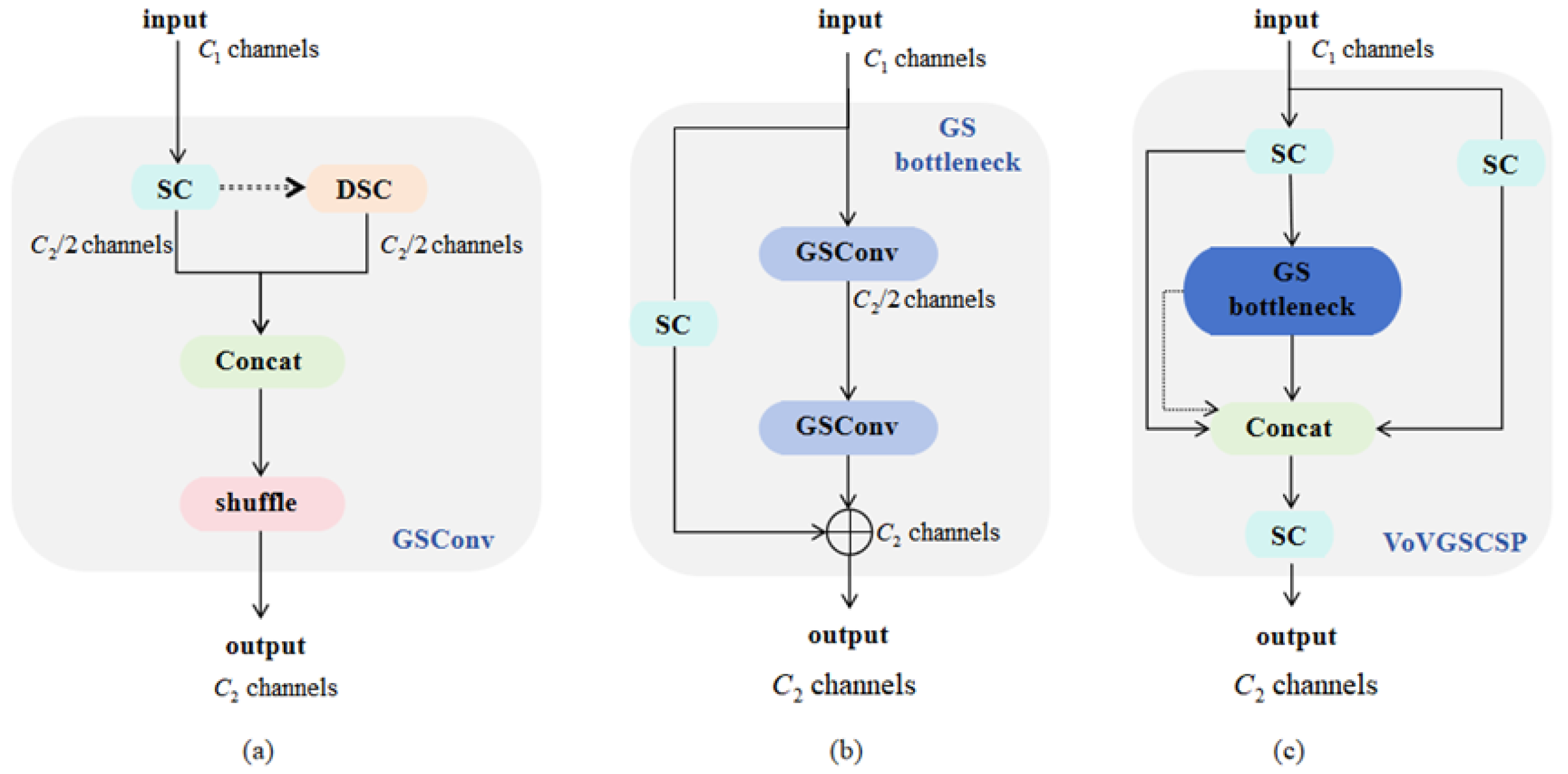
As illustrated in Figure 6c, the input features within the VoV-GSCSP module are initially split into two segments using the CSP strategy. One part is directly passed through a shortcut connection to retain the original information, while the other part is input into a module consisting of a bottleneck structure for further feature extraction. As shown in Figure 6b, the bottleneck structure integrates features processed by GSConv with those from the shortcut connection, resulting in higher-quality feature representations. GSConv combines DSC with SC, effectively lowering computational expenses while preserving precision. Additionally, the module employs shuffle operations to rearrange features across different channels, enhancing the information interaction between channels, as shown in Figure 6a.

The VoV-GSCSP module’s computational complexity is derived from a simplified GSConv formula. Under each convolution kernel, the grouping operation of input and output feature channels $C_1$ and $C_2$ are divided and manipulated, which significantly reduces the computational cost. The computation formula is as follows:

$$\mathrm{GFLOPs}\left(GSConv\right)=W·H·K_1·K_2·{\displaystyle \frac{C_2}{2}}·(C_1+1)$$

(11)

Here, W and H denote the feature map’s width and height, while $K_1$ and $K_2$ correspond to the convolution kernel dimensions. The input and output channels are represented by $C_1$ and $C_2$. Compared to standard convolution, the computational cost is reduced by approximately 50%. Moreover, by using channel grouping and shuffle operations, the nonlinear feature representation ability is preserved.

Overall, the VoV-GSCSP module successfully combines high performance with low computational cost through depthwise separable convolution, feature shuffle, and cross-stage partial aggregation strategies.

4. Experiments

This study aims to optimize the YOLOv11n model to enhance the accuracy and efficiency of steel surface defect detection. This section first introduces the experimental environment and evaluation criteria, including experimental settings, datasets, and evaluation metrics, which provide a unified foundation for subsequent experiments. Next, we conduct a comparative study of attention mechanisms to evaluate the impact of different attention modules on feature extraction capability and demonstrate the superiority of FCA in defect detection. Following this, a comparison of loss functions is performed to investigate the effect of various regression losses on the localization accuracy of small defects and assess the effectiveness of NWD in optimizing bounding box regression. Furthermore, an ablation study is conducted to analyze the independent contributions and combined effects of each proposed module (FCA, MSAF, NWD, VoV-GSCSP) to quantify their impact on detection performance. Finally, through a comprehensive model performance evaluation, FMV-YOLO is compared with state-of-the-art detection algorithms to validate its advantages in detection accuracy, computational efficiency, and practical industrial applications. These experiments are designed in a progressive manner, ensuring that each component’s effectiveness is thoroughly verified while demonstrating the overall optimization achieved by FMV-YOLO in steel surface defect detection.

4.1. Experimental Environment and Evaluation Criteria

4.1.1. Experimental Settings

In this paper, experiments were conducted on the proposed FMV-YOLO network across multiple datasets. The experimental hardware configuration comprised a 12th Gen Intel i5-12400F processor (2.50 GHz) and an NVIDIA GeForce GTX 3060 GPU. The model was trained using PyTorch 2.3.1 with CUDA 12.1 acceleration. Detailed parameter settings for the training process are provided in

Table 1. Specific parameter settings in the model training process.

Training Parameters	Details
Epochs	250
Image Size (pixels)	640 × 640
Batch Size	16
Workers	8
Initial Learning Rate ($l{r}_0$)	0.01
Final Learning Rate ($l{r}_f$)	0.001
Momentum	0.937
Mosaic	1.0
IoU Ratio ($\alpha$)	0.75
Optimization Algorithm	SGD

.

4.1.2. Dataset Description

This paper utilizes two types of datasets: one is a publicly available dataset, and the other is a self-constructed dataset from real industrial scenarios. We will conduct experiments on the publicly available dataset GC-DET to obtain the optimal model, and then perform generalization validation on another publicly available dataset, NEU-DET, as well as the self-constructed dataset LC-DET.

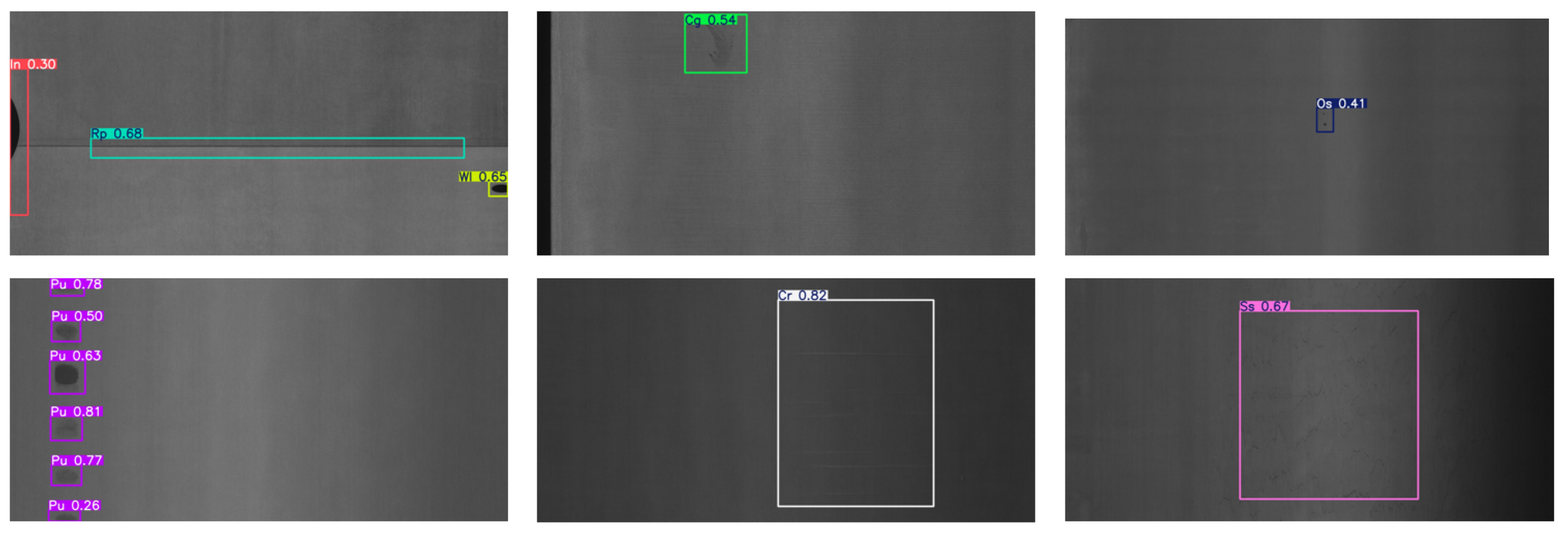
The publicly available dataset GC-DET is a steel surface defect dataset from Tianjin University. This dataset is a publicly available collection of steel surface defects obtained from real industrial scenarios, containing ten different types of defects, including Waist Fracture (Wf), Crescent Gap (Cg), Inclusion (In), Punching (Pu), Silk Spot (Ss), Water Spot (Ws), Oil Spot (Os), Rolling Pit (Rp), Crease (Cr), and Weld Line (Wl), totaling 2294 images. The publicly available dataset NEU-DET is a steel surface defect dataset from Northeastern University, focusing on six different types of defects, including Cracks (Cr), Inclusions (In), Patches (Pa), Pitted Surface (Ps), Rolled-in Scale (Rs), and Scratches (Sc), totaling 1800 images. To facilitate the validation of the proposed model’s performance, the datasets are divided in an 8:1:1 ratio.

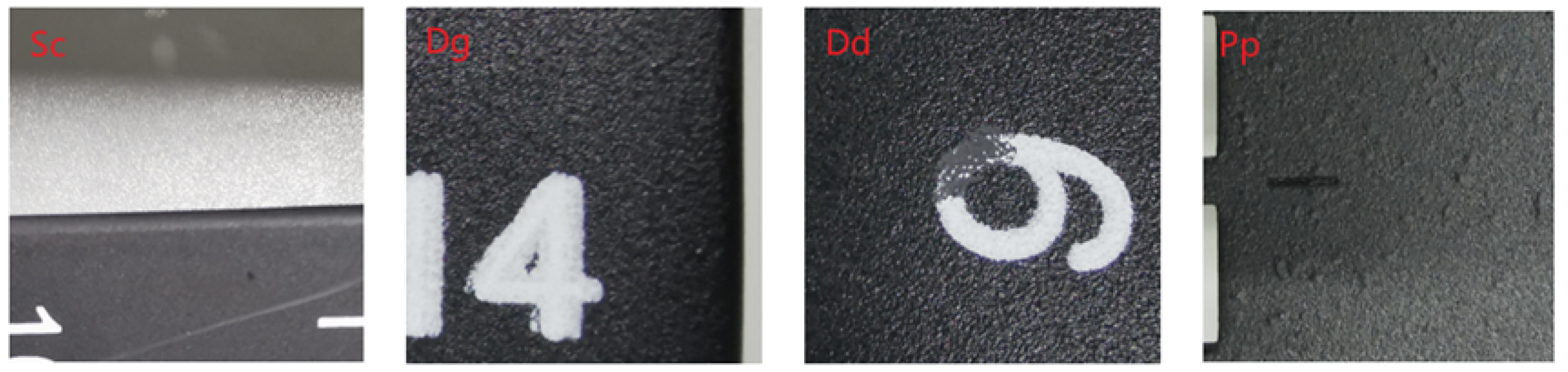
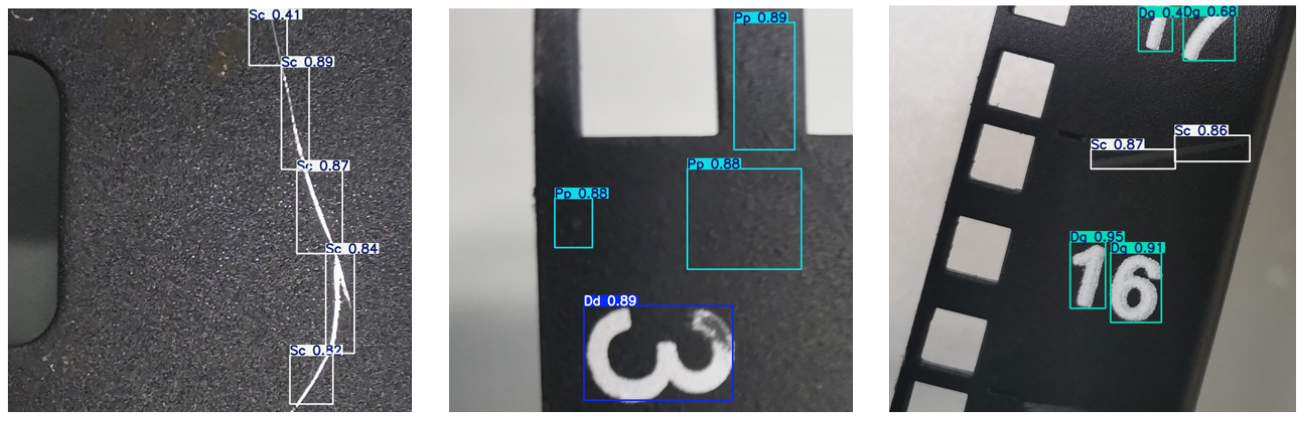
To address the problem of detecting steel defects in real industrial scenarios, we used a RealView camera (RER-USB4KHDRO1-V100, with a resolution of up to 3840 × 2160/30 fps) to capture numerous steel defect images at a hardware manufacturing company in Zhejiang. The original data were cropped and enhanced, and the dataset was named LC-DET. For dataset annotation, we used professional tools to precisely annotate defects in all images, with annotation files saved in YOLO format to facilitate seamless integration with detection models. Currently, this dataset includes the four most common types of defects encountered during the company’s production process: Scratches (Sc), Digital Printing Blurring (Dg), Digital Printing Defects (Dd), and Powder Accumulation (Pp). The entire dataset consists of 2397 images, showcasing diverse defect manifestations and covering complex industrial scenarios. Figure 7 provides example images of defect categories in LC-DET, visually illustrating the specific forms of various defects in the dataset. Scratches (Sc) appear as linear damage on the surface, Digital Printing Defects (Dd) represent quality issues in digital printing, Powder Accumulation (Pp) typically refers to material surface buildup, and Digital Printing Blurring (Dg) manifests as digital blurring or lack of clarity.

Figure 8 displays the distribution of instances in the GC-DET and LC-DET datasets, revealing a highly imbalanced distribution across different defect categories. This distribution reflects the real-world proportions and diversity of defects in actual industrial scenarios.

4.1.3. Evaluation Metrics

In this study, we employ commonly used evaluation metrics to comprehensively analyze model performance, focusing on the following four aspects:

• Precision (P) measures the proportion of samples predicted as positive that are actually positive, and it is used to assess the accuracy of predictions. The formula is given by the following:

  $$P={\displaystyle \frac{TP}{TP+FP}}\times 100\%$$

  (12)
• Recall (R) evaluates the proportion of actual positive samples that are correctly classified by the model, serving as an indicator of the model’s ability to detect all relevant instances:

  $$R={\displaystyle \frac{TP}{TP+FN}}\times 100\%$$

  (13)
• Average Precision (AP) evaluates the predictive performance for a single category by computing the area under the precision–recall curve:

  $$AP={\int }_0^{1}P\left(R\right)dR$$

  (14)
• Mean Average Precision (mAP) provides a comprehensive assessment by averaging AP values across all categories:

  $$mAP={\displaystyle \frac{1}{N}}\sum _{i=1}^{N}A{P}_i$$

  (15)

Additionally, to comprehensively evaluate the model, we analyze it from the perspective of model complexity, using parameter size (Params), computational cost (FLOPs), and frame rate (FPS), thereby assessing its resource consumption and practical applicability.

4.2. Experimental Analysis

4.2.1. Attention Mechanism Comparison Experiment

In the field of deep learning, attention mechanisms have become an indispensable technology due to their ability to dynamically allocate weights, enhance feature extraction capabilities, and reduce redundant information, thereby improving computational efficiency. However, different attention mechanisms have varying impacts on model performance. Therefore, selecting an appropriate attention module is crucial for optimizing detection tasks. The primary motivation of this experiment is to investigate the influence of various attention mechanisms on the YOLOv11 network and to verify the efficacy of the proposed FCAttention in object detection tasks.

We replaced the C2PSA in the YOLOv11 network with other attention mechanism modules (such as ECA [30], MCA [31], ABMLP [32], SE, and FCA) and conducted comparative experiments on the GC-DET dataset. The data are displayed in

Table 2. Comparison experiment of attention mechanisms.

Methods	P (%)	R (%)	mAP@0.5	mAP@0.5:0.95	Parameters	FLOPs (G)
YOLOv11n	73.4	65.2	69.5	33.3	2,584,102	6.3
+ECA	75.2	60.6	70.5	34.9	2,335,786	6.1
+MCA	71.0	67.0	70.4	34.6	2,335,792	6.1
+ABMLP	67.4	63.5	69.2	34.5	2,344,230	6.1
+SE	62.9	68.6	69.3	33.9	2,423,598	6.4
+FCA	72.2	68.2	71.2	35.3	2,401,580	6.1

The bolded labels indicate the best performance.

.

Through comprehensive comparative analysis, it was observed that replacing C2PSA with different attention mechanism modules improved the comprehensive performance of the model. This further confirms the importance of selecting an appropriate attention module for object detection tasks. Compared with the original C2PSA attention mechanism, FCAttention achieved the most significant performance improvement. Although the precision (P) decreased by 1.2%, the recall (R), mAP@0.5, and mAP@0.5:0.95 increased by 3.0%, 1.7%, and 2.0%, respectively. Additionally, the use of FCA reduced the model’s parameter count and computational cost. Therefore, replacing C2PSA with FCA in the YOLOv11 backbone network is more beneficial for the task addressed in this paper.

4.2.2. Comparison Experiment of Loss Functions

To explore the optimal bounding box regression strategy, this section conducts experimental comparisons of various mainstream loss functions (including CIoU [33], DIoU [34], GIoU [35], EIoU [36], SIoU [37], WIoU [38], Inner [39], and NWD loss). The aim is to verify whether the proposed NWD loss can outperform existing methods in terms of comprehensive performance and to investigate the impact of the hyperparameter $\alpha$ on its detection performance.

As shown in

Table 3. Comparison experiment of loss functions.

Algorithm	P (%)	R (%)	mAP@0.5	mAP@0.5:0.95
CIoU	73.4	65.2	69.5	33.3
DIoU	62.6	65.2	66.6	35.3
GIoU	65.9	68.0	69.1	34.5
EIoU	63.6	63.2	68.0	32.6
SIoU	71.2	63.0	69.6	35.8
WIoU	48.9	63.3	53.7	23.1
Inner	66.3	66.5	69.3	33.9
nwdloss ($\alpha$ = 0.35)	79.9	59.9	69.3	35.2
nwdloss ($\alpha$ = 0.55)	70.5	64.7	71.5	34.9
nwdloss ($\alpha$ = 0.75)	65.1	70.4	71.9	35.1

The bolded labels indicate the best performance.

, different loss functions significantly affect detection performance. CIoU and GIoU perform well on mAP@0.5, achieving 69.5% and 69.1%, respectively, but their performance on the more precise mAP@0.5:0.95 is relatively modest. DIoU and SIoU show improvements on mAP@0.5:0.95, reaching 35.3% and 35.8%, respectively, demonstrating advantages in optimizing high-quality bounding boxes. WIoU, due to its high sensitivity to hyperparameters, performs weakly overall, with mAP@0.5 at only 53.7%. In contrast, the proposed NWDLoss achieves the best comprehensive performance. When $\alpha$ (the weight of CIoU) is set to 0.75, mAP@0.5 reaches 71.9%, while recall reaches 70.4%, significantly outperforming other loss functions. These results demonstrate the effectiveness of NWDLoss in enhancing the model’s bounding box regression capability, providing new insights for optimizing loss functions in industrial detection tasks.

4.2.3. Ablation Experiment

To enhance object detection performance while balancing accuracy and computational cost, this paper optimizes the YOLOv11n network. The improvements include integrating Adaptive Fine-Grained Channel Attention (FCA) to strengthen feature extraction, employing Multi-Scale Attention Fusion (MSAF) to improve detection across different scales, utilizing the NWD loss to refine bounding box regression, and incorporating the VoVGSCSP module to enhance network architecture. To explore the independent contributions of these modules and their combined effects, this paper conducted ablation experiments on the public dataset GC-DET, with the specific results shown in

Table 4. Ablation experiment on GC-DET.

Model	P (%)	R (%)	mAP@0.5	mAP@0.5:0.95	Parameters	FLOPs (G)
YOLOv11n	73.4	65.2	69.5	33.3	2,584,102	6.3
+FCA	72.2	68.2	71.2	35.3	2,401,580	6.1
+MSAF	66.4	67.7	71.3	33.9	2,807,542	6.4
+NWD	65.1	70.4	71.9	35.1	2,584,102	6.3
+VoVGSCSP	77.3	62.4	70.7	34.5	2,603,382	5.8
+FCA+MSAF	67.2	70.4	71.7	35.3	2,625,020	6.2
+FCA+MSAF+NWD	71.3	68.6	73.7	35.9	2,625,020	6.2
FMV-YOLO	68.9	70.2	73.4	35.0	2,644,300	5.7

The bolded labels indicate the overall performance of the improved model in this paper.

.

Firstly, we independently introduced FCA, MSAF, NWD, and VoVGSCSP to verify the performance improvements brought by each module. Next, we progressively integrated these modules into the network to evaluate their combined effects. The experimental results show that the original YOLOv11n model achieved an mAP@0.5 of 69.5% and an mAP@0.5:0.95 of 33.3%, with FLOPs of 6.3G. Replacing C2PSA with FCA increased mAP@0.5 to 71.2% (+1.7%) and mAP@0.5:0.95 to 35.3% (+2.0%), while reducing FLOPs to 6.1G (−0.2G). On this basis, incorporating MSAF further improved mAP@0.5 by 0.5%, although FLOPs increased by 0.1G. Subsequently, after introducing NWD, mAP@0.5 increased by 2.0% and mAP@0.5:0.95 increased by 0.6%. Finally, after implementing all the improvements, the model achieved an mAP@0.5 of 73.4%, which is a 3.9% improvement over the original model. Meanwhile, the FLOPs reduced to 5.7G, representing an approximate 10% reduction. This confirms that the enhanced model improves detection precision while efficiently lowering computational overhead, increasing its suitability for mobile deployment.

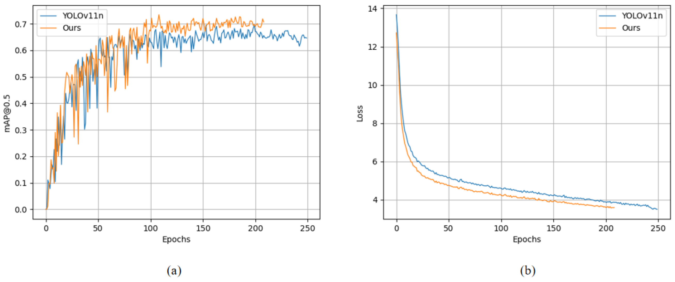
Figure 9 provides a comparative analysis of the base model YOLOv11n and the enhanced model FMV-YOLO during the training process. Figure 9a shows the variation in mAP@0.5, where the improved model performs similarly to the baseline in the first 50 epochs, with slight fluctuations. However, after 50 epochs, it gradually surpasses the baseline model and maintains higher detection accuracy in the later training stages. Figure 9b depicts the trend of the loss function, where the improved model exhibits a significantly faster reduction in loss during the early training phase compared to the base model, and it ultimately converges to a lower loss value, indicating faster convergence and superior optimization. Overall, the improved model outperforms the baseline YOLOv11n model in terms of both loss convergence speed and detection accuracy.

4.2.4. Model Performance Comparison

To verify the efficacy of the proposed FMV-YOLO model, we chose several mainstream models for comparison, focusing on their detection accuracy, recall rate, parameter count, and computational demand across different defect categories. This was performed to verify the advantages of the improved model in terms of accuracy and computational efficiency, and to assess its applicability in real-world industrial production environments.

The experimental outcomes of various models on the GC-DET dataset are displayed in

Table 5. Detection results for each defect in the GC-DET dataset.

Algorithm	Cr	Rp	Wf	Wl	In	Ss	Cg	Pu	Ws	Os
Faster R-CNN	45.8	12.9	63.7	72.4	22.5	73.1	80.0	83.4	70.3	55.2
Retina Net	40.2	43.9	87.0	91.5	29.7	66.4	94.3	79.6	79.1	62.0
YOLOv5n	65.6	34.8	89.6	92.9	28.0	67.0	97.5	98.4	72.5	69.4
YOLOv8n	62.5	15.9	85.8	91.2	30.1	63.1	92.3	96.9	74.0	73.2
YOLOv10n	43.1	14.9	85.0	88.7	28.2	56.7	87.8	94.4	73.5	57.5
YOLOv11n	54.1	43.3	90.1	88.2	22.2	61.0	96.7	97.0	77.8	64.2
WSS-YOLO [40]	58.1	35.4	93.4	95.2	38.0	62.8	93.5	98.7	57.9	59.7
Ours	69.7	54.8	88.8	81.9	28.2	63.5	94.1	96.3	80.7	76.3

The labels in bold denote the top performance, whereas the labels in blue signify the second-highest performance.

and

Table 6. Experimental results comparison on the GC-DET dataset.

Algorithm	P(%)	R(%)	mAP50	mAP50-95	Parameters	GFLOPs	FPS
Faster R-CNN	39.4	62.7	61.3	23.2	138.4M	368.2	26.3
Retina Net	40.9	65.1	67.5	32.7	31.6M	10.8	32.8
YOLOv5n	73.8	66.2	71.6	33.4	1,772,695	4.2	222.7
YOLOv8n	64.9	65.3	68.5	34.6	3,007,598	8.1	158.4
YOLOv10n	63.3	59.8	63.0	31.5	2,698,316	8.2	87.7
YOLOv11n	73.4	65.2	69.5	33.3	2,584,102	6.3	94.2
WSS-YOLO [40]	66.7	72.9	72.0	37.0	3,200,000	7.7	-
Ours	68.9	70.2	73.4	35.0	2,644,300	5.7	76.3

The labels in bold denote the top performance, whereas the labels in blue signify the second-highest performance.

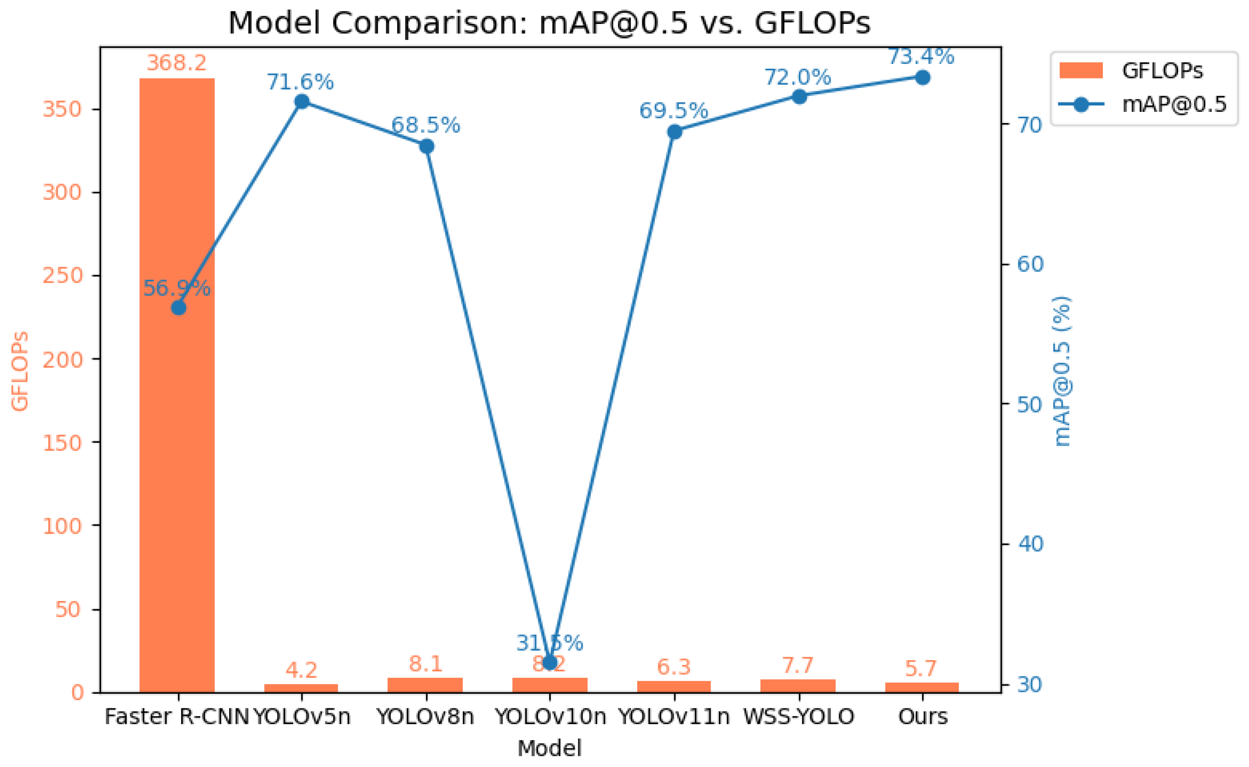
. Figure 10 shows their comparison in terms of mAP and computational load. It is clear that Faster R-CNN is at a disadvantage regarding accuracy and computational load. YOLOv5n and YOLOv8n achieve relatively good accuracy and recall rates with fewer parameters, but their detection results for certain defect categories (such as Ripple and Inclusion) still need improvement. In contrast, YOLOv10n and YOLOv11n show improved accuracy in some categories, but their overall mAP@0.5 does not have a significant advantage. WSS-YOLO performs notably well in recall and mAP@0.5, but its number of parameters and computational load are still high and require further optimization. Overall, our method maintains a comparatively small parameter count (approximately 2.64 M) and computational load (5.7 GFLOPs), while achieving 68.9% precision (P) and 70.2% recall (R), with mAP@0.5 at 73.4% and mAP@0.5:0.95 at 35%. It achieves high detection accuracy and recall rates across multiple defect categories, particularly showing robust performance in challenging areas such as Crack (Cr) and Ripple (Rp). With a frame rate of 76 fps, it is capable of real-time detection.

To further demonstrate the robustness of the proposed model in different scenarios, we conducted comparative experiments on another public dataset, NEU-DET. The experimental results are shown in

Table 7. Detection results for each defect on the NEU-DET dataset.

Algorithm	Cr	In	Pa	Ps	Rs	Sc
Faster R-CNN	40.0	77.1	91.6	72.7	63.4	95.7
Retina Net	45.9	84.2	91.1	87.4	58.6	81.5
YOLOv5n	40.9	80.1	93.3	79.7	62.1	86.4
YOLOv8n	47.8	82.6	93.9	84.9	60.2	94.1
YOLOv10n	44.9	77.3	93.4	85.1	64.5	89.0
YOLOv11n	45.3	82.4	95.2	88.0	68.4	93.3
WSS-YOLO [40]	58.1	80.9	93.9	94.2	73.1	93.9
Ours	52.6	84.7	96.7	86.7	67.3	93.4

The labels in bold denote the top performance, whereas the labels in blue signify the second-highest performance.

and

Table 8. Experimental results comparison on the NEU-DET dataset.

Algorithm	P	R	mAP50	mAP50-95	Parameters	GFLOPs	FPS
Faster R-CNN	34.8	90.2	72.9	33.5	138.4M	368.2	37.0
Retina Net	52.6	73.1	73.8	34.2	31.6M	10.8	41.2
YOLOv5n	66.8	71.7	73.7	39.0	1,767,283	4.2	204.7
YOLOv8n	75.2	72.5	77.2	44.2	3,006,818	8.1	154.9
YOLOv10n	72.5	69.6	75.7	43.1	2,696,756	8.2	93.2
YOLOv11n	74.8	72.8	78.8	45.0	2,583,322	6.3	106.6
WSS-YOLO [40]	76.0	75.6	82.3	47.0	3,200,000	7.7	-
Ours	77.7	73.0	80.2	44.90	2,644,300	5.7	96.5

The labels in bold denote the top performance, whereas the labels in blue signify the second-highest performance.

. It can be observed that our model achieves the best balance in terms of detection accuracy, parameter count, and computational cost. With only 2.64M parameters and a computational complexity of 5.7 GFLOPs, the model achieves an mAP@0.5 of 80.2% and an mAP@0.5:0.95 of 44.9%. Additionally, we applied this method to a real industrial scenario, achieving a precision (P) of 95.6%, a recall (R) of 96.4%, an mAP@.50 of 99%, an mAP@50:95 of 91.5%, and a frame rate of 94 fps on the LC-DET dataset, meeting the requirements of actual industrial production.

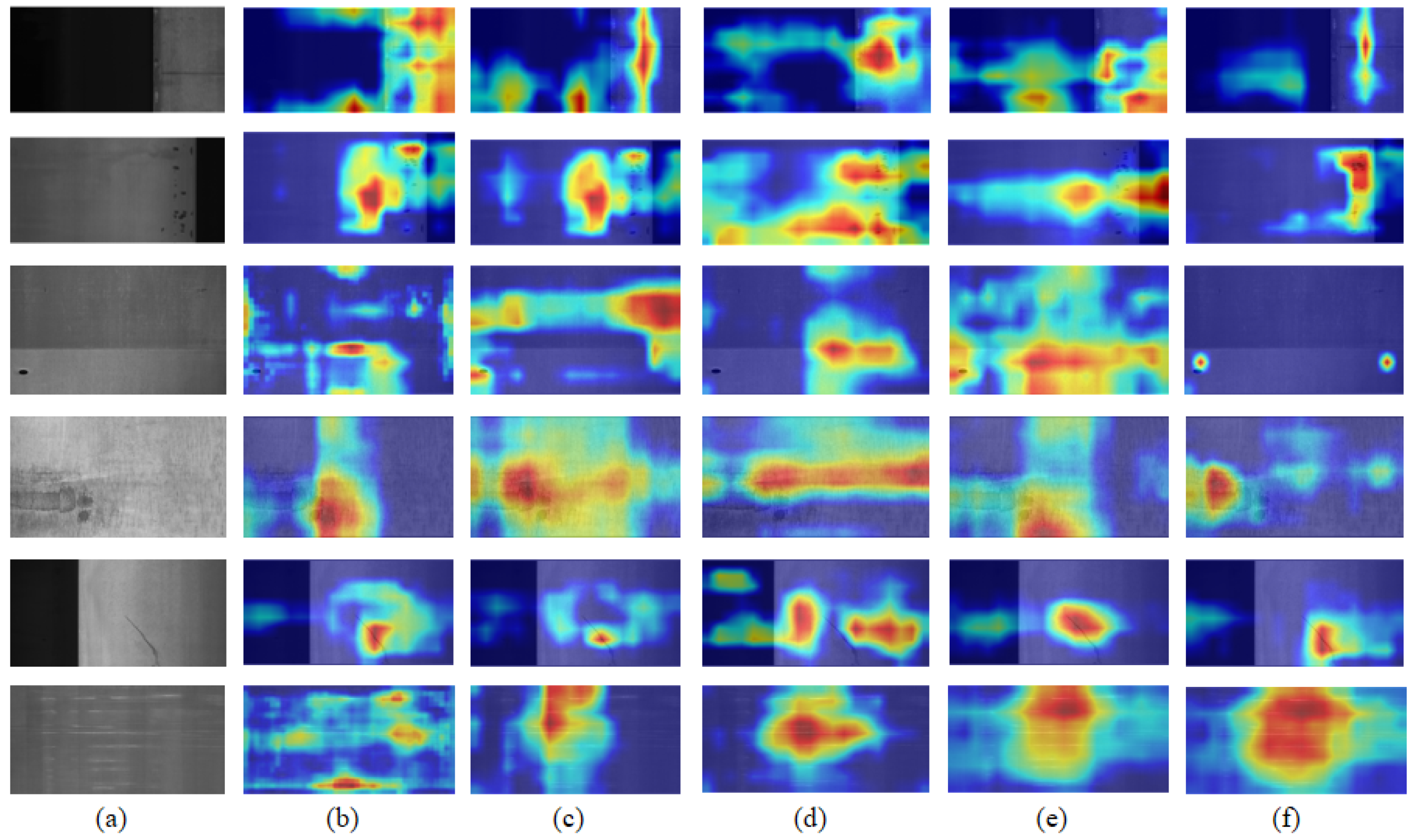
Finally, Figure 11 presents the heatmap visualization results of different models for the same set of steel surface defects. It can be observed that FMV-YOLO demonstrates more precise defect focus capabilities in heatmap visualization, enhancing small-target detection while reducing background interference. This indicates that FMV-YOLO, compared to YOLOv5n, YOLOv8n, YOLOv10n, and YOLOv11n, exhibits better feature representation capabilities in defect detection tasks, enhancing the practical application value of the model. Figure 12 and Figure 13, respectively, showcase the detection results of our method on the public dataset GC10-DET and the self-built dataset LC-DET. These visual results intuitively demonstrate the detection capabilities of the improved model in practical applications, validating its utility and reliability in steel surface defect detection tasks.

In summary, through quantitative performance metrics and qualitative visual comparisons, our method outperforms existing mainstream models across multiple key performance indicators and demonstrates exceptional detection capabilities and efficient computational performance in real industrial application scenarios. This indicates that our improved model has broad application prospects and significant advantages in the field of steel surface defect detection, effectively enhancing the quality control level of industrial production, reducing the occurrence of defective products, and improving production efficiency.

5. Discussion and Conclusions

5.1. Discussion

To achieve accurate detection of steel surface defects, this paper proposes an improved detection algorithm, FMV-YOLO, based on YOLOv11n, and validates its effectiveness on both publicly available and self-constructed datasets. First, to enhance the model’s capability in detecting steel surface defects, we replace the C2PSA attention module in the backbone network with an Adaptive Fine-Grained Channel Attention (FCA) mechanism, enabling the model to better integrate global and local information and capture key features more precisely. Second, to address the fusion of multi-scale defect features, we introduce a Multi-Scale Attention Fusion (MSAF) module, which effectively improves the model’s adaptability to defects of different scales and variations. Third, to enhance the model’s localization accuracy for small defects, we optimize the loss function by employing a weighted combination of the Normalized Wasserstein Distance (NWD) and IoU, refining the bounding box regression strategy. Finally, to meet real-time detection requirements in industrial applications, we incorporate the VoV-GSCSP module into the neck network, significantly reducing computational complexity and parameter count, achieving a lightweight design.

On the GC-DET dataset, FMV-YOLO, with 2.64M parameters and 5.7 GFLOPs, outperforms most models in mAP@0.5 (73.4%) and mAP@0.5:0.95 (35%), demonstrating robust performance in challenging defect categories such as Crack (Cr) and Ripple (Rp). In contrast, YOLOv5n and YOLOv8n exhibit better parameter efficiency but show suboptimal performance in certain defect categories, while WSS-YOLO achieves superior recall and mAP but has a higher computational cost, making it less suitable for real-time applications. On the NEU-DET dataset, FMV-YOLO achieves an mAP@0.5 of 80.2% and an mAP@0.5:0.95 of 44.9%, performing comparably to WSS-YOLO but with lower computational requirements, making it more suitable for industrial deployment. Furthermore, on the LC-DET real-world industrial dataset, FMV-YOLO achieves 95.6% precision, 96.4% recall, and 99% mAP@0.5, with an inference speed of 94 FPS, fully meeting the real-time detection requirements of industrial applications. The visualization results further demonstrate that FMV-YOLO can accurately identify various defects and maintain high detection precision even in complex backgrounds, highlighting its practical applicability and robustness in real-world defect detection tasks.

5.2. Conclusions

Overall, FMV-YOLO outperforms existing mainstream models across multiple key performance metrics, achieving a well-balanced trade-off between detection accuracy, computational complexity, and model lightweighting. In particular, for small object detection and complex background scenarios, the integration of FCA, MSAF, and NWD significantly enhances detection robustness, while the incorporation of the VoV-GSCSP lightweight design effectively reduces computational costs, meeting the real-time and high-reliability requirements of industrial production.

However, there is still room for further optimization. First, regarding the detection of rare defect categories, the imbalanced distribution of defect types in industrial datasets may lead to performance degradation. Future research could explore data augmentation and synthetic data generation to improve the model’s learning capability. Second, in terms of small object detection accuracy, although NWD has optimized bounding box regression, further enhancements could be achieved by adopting ensemble learning methods, such as fusing multiple optimized YOLO variants or integrating features from different models, to enhance the robustness and generalization capability of the detection system.

In conclusion, FMV-YOLO demonstrates outstanding potential in industrial defect detection, offering an effective solution for improving quality control in industrial production, reducing defective products, and increasing manufacturing efficiency. It provides a reliable and efficient approach for intelligent manufacturing and automated defect detection, contributing to the advancement of real-time and high-precision industrial inspection systems.