Local Batch Normalization-Aided CNN Model for RSSI-Based Fingerprint Indoor Positioning

Abstract

Indoor positioning systems have become increasingly important due to the limitations of GPS in indoor environments, such as non-line-of-sight conditions and weak signal strength. Among the various indoor positioning techniques, fingerprinting-based approaches utilizing WiFi signals are highly regarded for their accessibility and convenience. However, existing convolutional neural network (CNN) models for fingerprinting often struggle to maintain consistent performance under diverse environmental conditions. To address these challenges, this study proposes a local batch normalization (LBN)-aided CNN model for received signal strength indicator (RSSI)-based indoor positioning. The LBN technique is designed to overcome the limitations of traditional batch normalization (BN) and layer normalization (LN) in managing location-dependent RSSI variations, thereby improving positioning accuracy. The proposed approach consists of two phases: an offline phase, where RSSI data are collected at reference points to train the model, and an online phase, where real-time RSSI data are used to estimate the device’s location. Experimental results demonstrate that the proposed LBN-aided CNN model achieves an accuracy of 92.9%, outperforming existing CNN-based methods. These findings confirm the effectiveness of LBN in enhancing CNN performance for indoor positioning, particularly in challenging environments with significant signal variability.

1. Introduction

The increasing reliance on location-based services in GPS-weak or unavailable environments, such as indoor spaces, has driven significant demand for indoor positioning systems across various settings. These include hospitals, shopping malls, prisons, warehouses, factories, and underground parking lots [1,2,3]. Among wireless signal-based positioning techniques, the received signal strength indicator (RSSI) is widely used due to its simplicity and cost-effectiveness. RSSI leverages the relationship between signal strength and distance, making it an attractive option for indoor localization. However, RSSI-based methods face inherent challenges due to the instability of RSSI measurements [4]. Dynamic environmental factors, such as human movement, equipment-generated noise, and changes in antenna orientation, significantly disrupt RSSI readings [5,6]. Additionally, multipath fading, time-varying signal characteristics, and uneven RSSI data distributions introduce substantial noise, complicating the development of robust models [7].

Traditional indoor positioning methods, such as trilateration and the weighted centroid localization algorithm, also have limitations [8,9,10]. Trilateration accuracy is degraded by obstacles, while traditional methods often overlook factors such as height differences between access points (APs) and terminals, leading to significant positioning errors, particularly in multi-story buildings [11]. In contrast, machine learning approaches, particularly convolutional neural networks (CNNs), have shown potential in improving the accuracy of RSSI-based indoor positioning systems [12]. However, CNNs also face challenges, such as handling uneven data distributions and localized feature variations, which can impact predictive stability. Environmental noise and dynamic changes, such as multipath effects, contribute to data inconsistencies, reducing positioning accuracy [13,14,15]. CNNs further struggle with classification near region boundaries, and their effectiveness depends heavily on large, high-quality training datasets.

Batch normalization (BN), introduced by Ioffe and Szegedy in 2015, addresses some of these challenges by normalizing the mean and variance of activations within a mini-batch, stabilizing the input distribution during training [16]. This process mitigates internal covariate shifts, accelerates convergence, and supports the use of higher learning rates without risking divergence. BN enhances gradient flow, particularly in deep architectures, by incorporating learnable parameters that preserve the network’s representation capacity. Additionally, BN serves as an effective regularizer, facilitates the use of non-linear activation functions, and mitigates saturation issues, improving CNN performance in various applications, including indoor positioning [17]. However, theoretical analyses of BN often rely on simplified assumptions that fail to capture the complexities of modern deep neural network (DNN) training [18]. BN is also sensitive to uneven data distributions and local feature variations, which can limit its effectiveness in noisy and dynamic environments [19].

To address the limitations of BN, several alternative normalization techniques have been developed. Layer normalization (LN), proposed by Lei Ba et al., normalizes across all features for each training example, making it particularly effective for recurrent neural networks by stabilizing their hidden state dynamics [20]. Instance normalization (IN), introduced by Ulyanov et al., normalizes each channel independently for each sample, excelling in tasks like style transfer due to its ability to capture fine-grained local statistics [21]. Group normalization (GN), developed by Wu and He, divides channels into groups and normalizes within each group, demonstrating superior performance in tasks with small batch sizes, such as object detection and video classification [22]. Within the context of these methods, LN was chosen as a representative alternative normalization technique for comparative analysis in our ablation study. While these methods aim to stabilize training and improve generalization, they often struggle in scenarios with highly localized feature variations, such as RSSI-based indoor positioning systems, where signal strength significantly varies across locations.

Motivated by the need to enhance CNN performance in RSSI-based indoor positioning, this study introduces a novel local batch normalization (LBN) technique designed to address the challenges of uneven data distributions and localized feature variability. RSSI data often exhibit significant non-independent and identically distributed (non-IID) characteristics due to spatial dependencies, temporal fluctuations caused by dynamic environmental changes, and localized variations introduced by obstacles and noise. These properties lead to uneven data distributions, increasing the complexity of training models and exposing the limitations of traditional BN techniques. The proposed LBN approach normalizes inputs at a more localized level, enabling the model to better handle signal fluctuations and enhancing the generalization ability of the CNN model in dynamic environments. By specifically targeting location-dependent feature variations, LBN aims to improve the robustness of RSSI-based indoor positioning systems under irregular distributions and environmental noise.

This paper is organized as follows: Section 2 provides background information, including an overview of BN and LN, and their limitations. Section 3 presents the proposed LBN-aided positioning scheme, detailing the methodology and CNN architecture. Section 4 introduces the simulation setup, experimental design, and data processing and analyzes the results by comparing the performance of the baseline CNN model with those incorporating BN, LN, and LBN. Finally, Section 5 concludes the study by summarizing key findings and suggesting future research directions.

2. Background

2.1. Batch Normalization and Its Limitations

BN is a technique used to accelerate and stabilize the training of neural networks. It works by normalizing the inputs to each layer based on the statistics of a mini-batch, thereby mitigating internal covariate shift. This process not only speeds up training but also allows for the use of higher learning rates. Since its introduction, BN has been widely adopted in various network architectures, including ResNet [23] and Inception [24]. However, BN has some limitations, particularly its sensitivity to small batch sizes, which has led to the development of alternative normalization techniques. One such alternative is LN [20], which standardizes across the features rather than the batch dimension, making it more suitable for recurrent neural networks. Another alternative is GN [22], which divides features into groups, striking a balance between batch and layer normalization.

The core idea behind BN, as introduced by Ioffe and Szegedy [16], is the standardization of layer inputs during the training phase to address internal covariate shift in deep neural networks. This process, outlined in Section 8.7.1 of Deep Learning by Goodfellow et al. [25], involves the following key steps:

• Calculate the mean and variance: Compute the mean and variance for each mini-batch.

$${\mu }_{batch}={\displaystyle \frac{1}{m}}\sum _{i=1}^m{x}_i, {\sigma }_{batch}^2={\displaystyle \frac{1}{m}}\sum _{i=1}^m{\left(x_i-{\mu }_{\mathrm{b}\mathrm{a}\mathrm{t}\mathrm{c}\mathrm{h}}\right)}^2$$

(1)

2.

Normalize: Standardize the inputs using the calculated mean and variance to achieve zero mean and unit variance.

$$\widehat{x}={\displaystyle \frac{x-{\mu }_{batch}}{\sqrt{{\sigma }_{batch}^2+ϵ}}}$$

(2)

3.

Scale and shift: Introduce two learnable parameters, the scale factor (γ) and the shift factor (β), to adjust the normalized data. These adjustments allow the network to maintain its representational capacity.

$$y=\gamma \widehat{x}+\beta ,$$

(3)

Variable Definitions:

$x_i$ is the input of the i-th sample in a mini-batch.

$x$ is the input value before normalization.

$\widehat{x}$ is the normalized input.

${\mu }_{batch}$ is the mean of the mini-batch.

${\sigma }_{batch}^2$ is the variance of the mini-batch.

$m$ is the number of samples in the mini-batch.

$ϵ$ is a small constant added to prevent division by zero.

$y$ is the final output of the BN process.

$\gamma$ and $\beta$ are learnable parameters that scale and shift the normalized data, respectively.

2.2. Layer Normalization and Its Limitations

In their work, Lei Ba et al. proposed layer normalization (LN) as a method to normalize the summed inputs within a hidden layer. The process is independent of mini-batch statistics [20]. Distinct from batch normalization (BN), which normalizes data batch-wide mean and variance, LN computes statistics for each individual training instance separately. This independence from batch size allows LN to be effectively applied to various neural network architectures, including models where batch statistics are unreliable, such as recurrent neural networks (RNNs).

The core mathematical process of LN involves computing the mean and standard deviation for all neurons in a layer for each individual training case. The key steps are as follows:

• Calculate the Mean and Standard Deviation: Compute the mean ${\mu }^l$ and standard deviation ${\sigma }^l$ across all hidden units in a layer for a given training instance:

  $${\mu }^l={\displaystyle \frac{1}{H}}\sum _{i=1}^H{a}_i^l, {\sigma }^l=\sqrt{{\displaystyle \frac{1}{H}}\sum _{i=1}^H{\left(a_i^l-{\mu }^l\right)}^2}$$

  (4)
• Normalize: Standardize the inputs using the computed statistics to ensure zero mean and unit standard deviation:

  $${\widehat{a}}_i^l={\displaystyle \frac{a_i^l-{\mu }^l}{{\sigma }^l+ϵ}}$$

  (5)
• Scale and Shift: Introduce learnable parameters, the scale factor γ and the shift factor β, to adjust the normalized activations:

  $$y_i^l=\gamma {\widehat{a}}_i^l+\beta ,$$

  (6)

The parameters μl and σl were introduced by Lei Ba et al. [20] as part of the LN method, while ${\widehat{a}}_i^l$ and $y_i^l$ represent general normalized activations and outputs, respectively.

Variable Definitions:

$a_i^l$ is the summed input to the i-th neuron in layer l.

${\widehat{a}}_i^l$ is the normalized activation of the i-th neuron in layer l.

${\mu }^l$ is the mean of all neurons in layer l.

${\sigma }^l$ is the standard deviation of all neurons in layer l.

$H$ represents the number of hidden units in the layer, rather than the mini-batch size.

ϵ is a small constant added to prevent division by zero.

$y_i^l$ is the final output of the LN process for the i-th neuron in layer l.

$\gamma$ and $\beta$ are learnable parameters that scale and shift the normalized data, respectively.

In contrast to BN, where γ and β are learned on a per-feature-channel basis, LN applies a single γ and β across all neurons within a layer. LN provides several advantages over BN. By eliminating the reliance on batch-dependent statistics, LN maintains its effectiveness even when dealing with models trained using small batch sizes or in an online learning setting. LN is also beneficial in architectures like RNNs, where it helps stabilize training and mitigate issues such as exploding and vanishing gradients. Recent studies suggest that layer normalization has limitations in certain architectures. In particular, modified layer normalization (MLN) has been shown to offer improvements in specific settings [26]. Moreover, layer normalization has been found to be less effective than self-normalizing networks (SNNs) in some contexts [27]. These findings indicate that the effectiveness of normalization techniques can be highly architecture-dependent, with different methods excelling in distinct scenarios.

3. Proposed LBN-Aided Positioning Scheme

3.1. Local Batch Normalization

BN has been widely recognized for its effectiveness in enhancing the performance of positioning systems across various network architectures, such as the improved residual network (ResNet) [28] and the multi-path res-inception (MPRI) network [29]. However, despite its strengths, BN has limitations. Its performance can degrade when faced with uneven data distributions [30] or small batch sizes [22]. Additionally, BN’s reliance on batch-level statistics becomes problematic in non-independent and identically distributed (non-IID) data settings [31]. 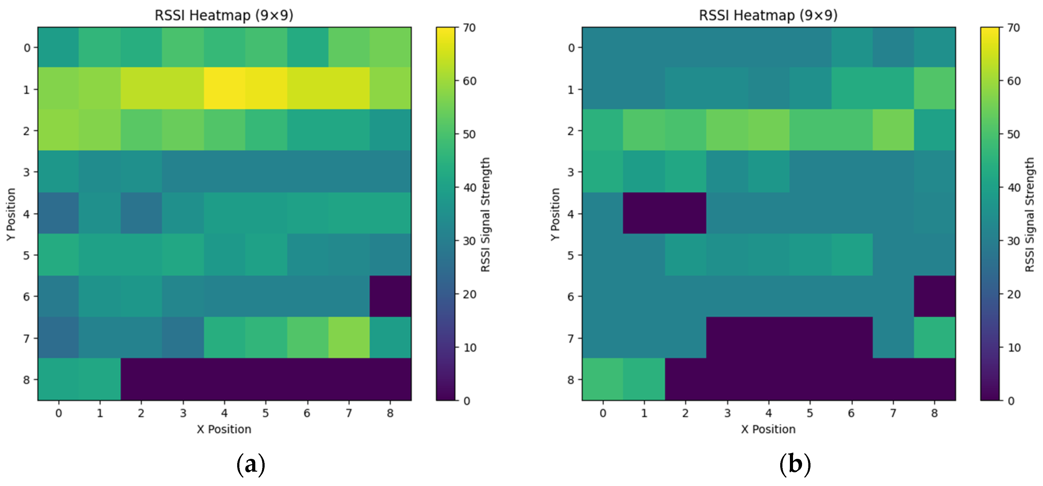These limitations are especially evident in scenarios like RSSI-based positioning, where the data exhibit non-IID characteristics [32] due to spatial dependencies, temporal variations, and environmental noise. This highlights the need for more robust normalization techniques. Figure 1 illustrates RSSI heatmaps for two WiFi access points, revealing spatial dependencies and uneven signal distributions that reflect the non-IID nature of the data.

To address these challenges, Li et al. introduced local batch normalization (FedBN) for federated learning, a specific adaptation of batch normalization (BN) designed to mitigate feature shift [31]. Unlike traditional BN, which aggregates normalization parameters across all clients, FedBN retains parameters locally on each client, ensuring the normalization process aligns with the specific data distribution of each client. This approach has proven effective in mitigating feature heterogeneity, improving both convergence rates and model performance in federated learning scenarios [31]. The key aspects are as follows:

• Compute Local Batch Normalization Statistics: Adhering to the BN formulation detailed in Section 2.1, FedBN modifies the normalization procedure by computing the mean and variance locally for each individual client. Specifically, the mean and variance are calculated as follows:

$${\mu }_c={\displaystyle \frac{1}{m}}\sum _{i=1}^m{x}_i,{\sigma }_c^2={\displaystyle \frac{1}{m}}\sum _{i=1}^m{\left(x_i-{\mu }_{\mathrm{c}}\right)}^2$$

(7)

2.

Normalize Using Local Statistics: Each client normalizes activations using its local statistics to ensure consistency within its own feature distribution:

$${\widehat{x}}_i={\displaystyle \frac{x_i-{\mu }_c}{\sqrt{{\sigma }_c^2+ϵ}}}$$

(8)

3.

Scale and Shift Using Learnable Parameters: Following the standard BN formulation, each client incorporates learnable scale and shift parameters to restore the network’s representational capacity:

$$y_i={\gamma }_c{\widehat{x}}_i+{\beta }_c,$$

(9)

4.

Global Model Aggregation (Excluding BN Parameters)

FedBN modifies the federated learning model aggregation process by ensuring that only non-BN parameters are synchronized across clients. The BN parameters ${\mu }_c$, ${\sigma }_c^2$ remain client-specific and are excluded from model averaging. This adaptation ensures that each client retains its own batch statistics. By doing so, it allows FedBN to effectively handle feature shift while still enabling clients to benefit from federated model training.

Variable Definitions:

$x_i$ is the input of the i-th sample in a mini-batch.

${\widehat{x}}_i$ is the normalized activation of the input.

$m$ is the number of samples in the mini-batch,

${\mu }_c$ is the mean of the batch normalization layer computed locally on client c.

${\sigma }_c^2$ is the variance of the batch normalization layer computed locally on client c.

$ϵ$ is a small constant added to prevent division by zero.

$y_i$ is the final output of the FedBN process for the i-th sample.

${\gamma }_c$ and ${\beta }_c$ are learnable parameters that scale and shift the normalized data, respectively.

FedBN’s principles provide a valuable foundation for addressing distributional disparities in RSSI-based indoor positioning. When applied directly to CNN models for indoor localization, traditional BN fails to account for localized variations, leading to reduced robustness and accuracy.

Building on the concepts of FedBN, this study proposes an LBN technique specifically designed for RSSI-based indoor positioning systems. Unlike FedBN, which operates within a federated learning framework, the proposed LBN is integrated directly into a CNN model, optimizing it for the specific challenges of RSSI signal processing. By applying normalization at a localized level, aligned with the spatial and positional characteristics of RSSI data, LBN enhances the model’s sensitivity to location-specific features. This improves overall positioning accuracy and robustness. In doing so, LBN overcomes the limitations of traditional BN in indoor localization, offering a pathway to more accurate and reliable positioning systems.

3.2. LBN for RSSI-Based Indoor Positioning

Building on existing normalization techniques, we propose a novel approach called LBN, specifically designed for RSSI signal-based indoor positioning. The LBN technique divides the input feature map into spatially localized patches, applying normalization within each patch. This localized strategy allows the model to better capture variations in RSSI signal distributions, thereby improving its performance in indoor localization tasks.

As shown in the pseudocode in Algorithm 1, the method operates as follows:

• LBN divides the input tensor into non-overlapping spatial patches of size block_size × block_size, performing localized normalization within each patch.
• The technique involves initializing learnable scaling (γ) and shifting (β) parameters, set to 1 and 0, respectively. Additionally, momentum and epsilon (ϵ) are introduced to control the moving averages and ensure numerical stability.
• During forward propagation, LBN extracts the input tensor dimensions, including batch size, height, width, and number of channels, and calculates the block dimensions (block_h and block_w) to divide the input into patches.
• For each patch, localized mean and variance are computed to enable normalization specific to the spatial region.
• In training mode, patches are normalized using the calculated statistics:

$$normalized\_patch={\displaystyle \frac{(patch-mean)}{\sqrt{(variance+ϵ)}}}$$

(10)

6.

The patches are then reshaped to their original dimensions.

7.

Scaling and shifting are applied:

$$output=\gamma ·normalized\_patch+\beta$$

(11)

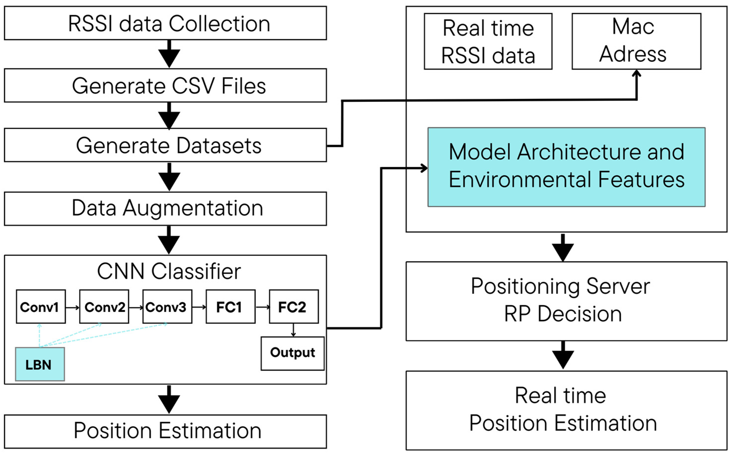
During inference, precomputed moving averages of the mean and variance are used to ensure stable predictions. By incorporating spatial locality into the normalization process, LBN enhances the CNN’s ability to learn localized features, improving the model’s robustness and positioning accuracy. LBN is applied within the CNN model, as shown in Figure 2.

Algorithm 1 Localized Batch Normalization
1.	Input: Input tensor inputs, Block size block_size, Momentum momentum, Epsilon ε
2.	Initialize: Trainable weights γ and β for each channel
3.	Extract input dimensions: batch_size, height, width, channels
4.	Compute block dimensions: block_h = height // block_size, block_w = width // block_size
5.	Divide input into block_size × block_size patches
6.	Compute mean and variance for each patch
7.	if training mode then
8.	Normalize patches: (patch – mean) /$\sqrt{(variance+\epsilon )}$
9.	end if
10.	Reshape patches to original dimensions
11.	Apply weights: outputs = γ · patches + β
12.	Return: Normalized output tensor outputs

3.3. CNN Model and Data Processing

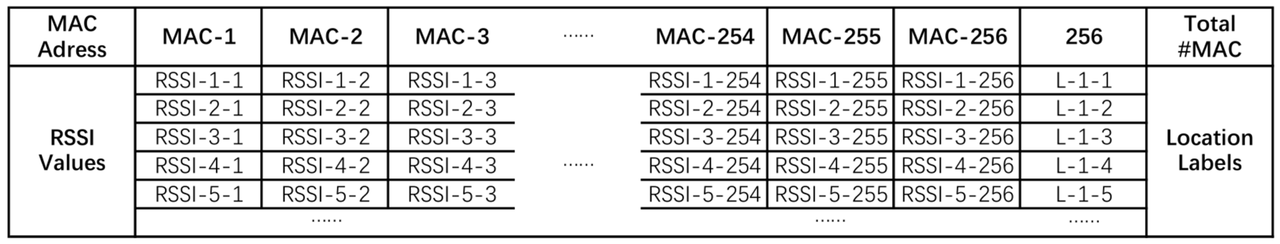
This section details the preprocessing of collected RSSI data and its use as input for the CNN model. Initially, the RSSI data are collected and transmitted to the server in a .txt file format. It is then converted into a comma-separated values (CSV) file, which serves as the input for the CNN model. As shown in Figure 3, the CSV file contains location-specific information, including the media access control (MAC) addresses of APs, their corresponding RSSI values, and the quantities recorded at each location. The MAC address information is represented by the blue box in the CSV file, with a maximum capacity of 256 MAC addresses. Each CSV file consists of 257 columns, where columns 1 to 256 represent RSSI values, and the 257th column indicates the category (e.g., location label). There are 74 distinct categories in total. Each row contains 256 RSSI values, corresponding to signals received from various WiFi sources at a specific RP.

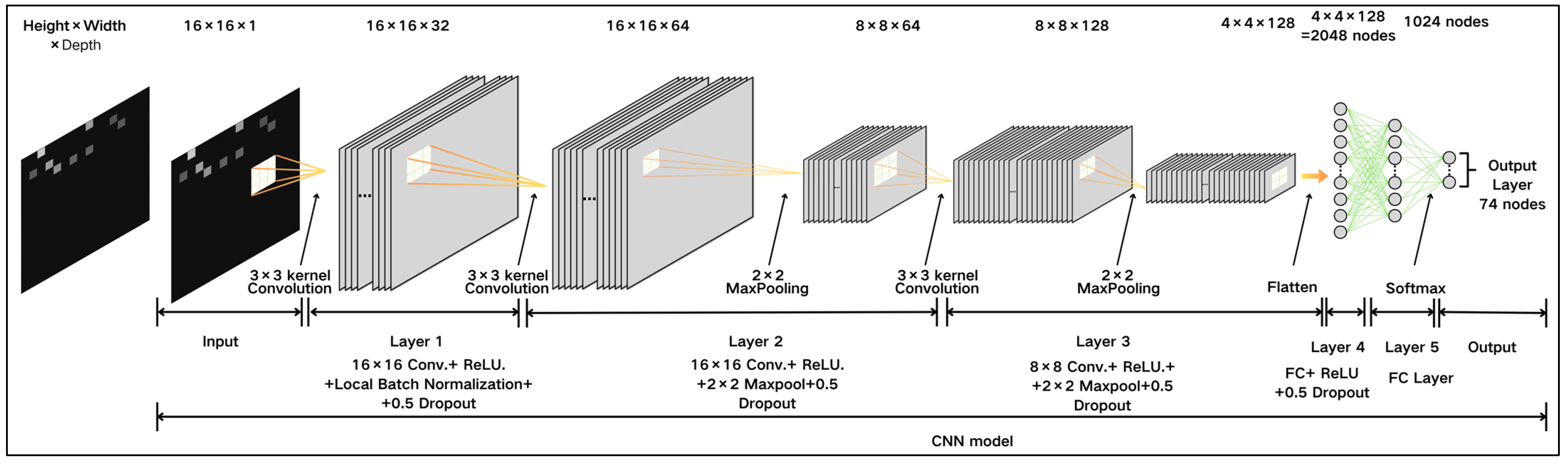
Figure 4 provides a detailed overview of the CNN model architecture used in this study. The model is structured into five layers as follows:

• Input Layer (First Layer): Accepts a 16 × 16 × 1 grayscale image, applies a Rectified Linear Unit (ReLU) activation function, LBN, and implements a dropout rate of 0.5.
• Second Layer: Contains 16 × 16 convolutional filters, ReLU activation, an 8 × 8 max-pooling layer, and a dropout rate of 0.5, with a total of 18,496 parameters.
• Third Layer: Includes 8 × 8 convolutional filters, ReLU activation, a 4 × 4 max-pooling layer, and a dropout rate of 0.5, with 73,856 parameters.
• Fourth Layer: A fully connected (FC) layer with 2048 nodes, resulting in 2,098,176 parameters.
• Fifth Layer: Another FC layer with 1024 nodes, totaling 76,875 parameters. The outputs are calculated using a softmax layer with 74 nodes, corresponding to the total number of RPs.

The model uses a learning rate of 0.001 and has a total of 2,267,851 parameters. LBN is applied at every layer where traditional batch normalization is typically used. This technique normalizes local distributions to adapt to the spatial heterogeneity of RSSI data, enhancing feature sensitivity and improving robustness across varied inputs. A summary of all parameter settings is provided in

Table 1. Hyperparameter settings for the CNN model.

Description	Our CNN Models
Input Size	16 × 16
Number of Convolutional Layers	3
Filter Size	3
Number of Feature Maps	32–128
Pooling Size	2
Learning Rate	0.001
Batch Size	200
Stride	1
Number of FC Layers	2
Total Weights	4.50 million

. The primary objective of data augmentation is to improve the model’s generalization to unseen data. The strategy employed is based on the method proposed by Rashmi et al. [9], designed to generate additional RPs and expand the dataset significantly. Each row of the CSV file, containing 256 RSSI values, is transformed into a 16 × 16 grayscale image for processing in the CNN model. The leftmost image in Figure 4 illustrates an example of a generated image. In these images, darker regions represent stronger RSSI signals, while lighter regions indicate weaker signals. If the RSSI value is 0, no brightness is generated. The original dataset comprises 7008 images for the training set. After applying data augmentation, this number increases to 427,488 images. The test set includes 1110 images.

4. Numerical Results

4.1. Simulation and Experiment Setup with Data Processing

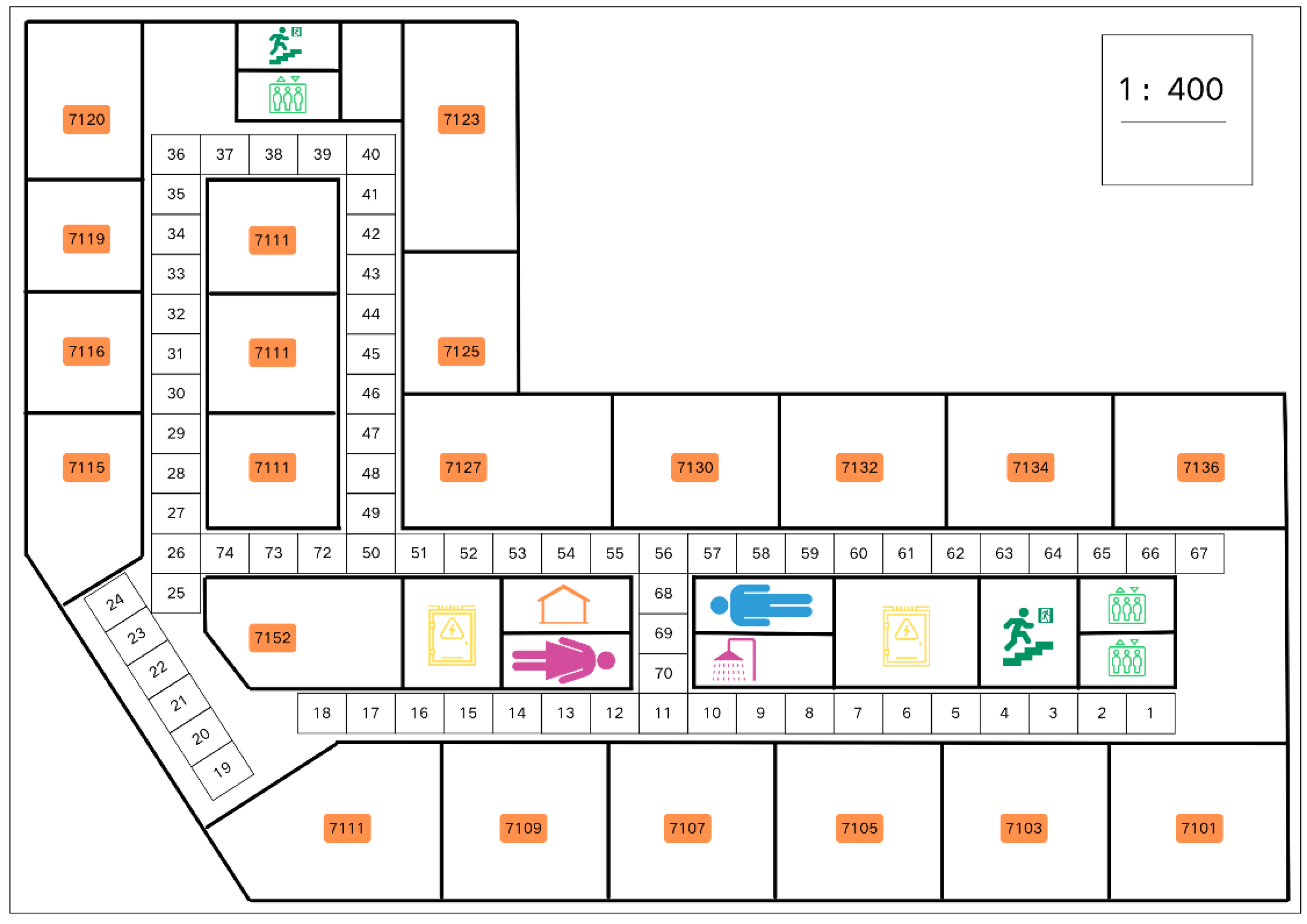
The data collection, simulation tests, and experimental tests were conducted on the 7th floor of the New Engineering Building at Dongguk University. This environment facilitated the generation of an RSSI fingerprint dataset. As shown in Figure 5, 74 reference points (RPs) were designated, with a 2-m interval between each RP.

On the hardware side, a Samsung SHV-E310K smartphone (Samsung Electronics, Suwon, Republic of Korea), a MAP200N high-performance wireless device (HPOWD) (JMP SYSTEM, Korea), and a Dell Alienware Model P31E (Dell Inc., Round Rock, TX, USA) were used. During the data collection and processing phase, the smartphone collected RSSI signals. These signals were then transmitted to the computer through the HPOWD for storage. The computer then performed database construction, data preprocessing, data augmentation, and CNN training. In the positioning phase, the smartphone was placed on a height-adjustable stand. This was performed to ensure accurate and precise positioning. Subsequently, the smartphone collected RSSI signals in real time. After that, it transmitted these signals to the computer via the HPOWD. Once the computer received the data, it processed the data and finally displayed the positioning results.

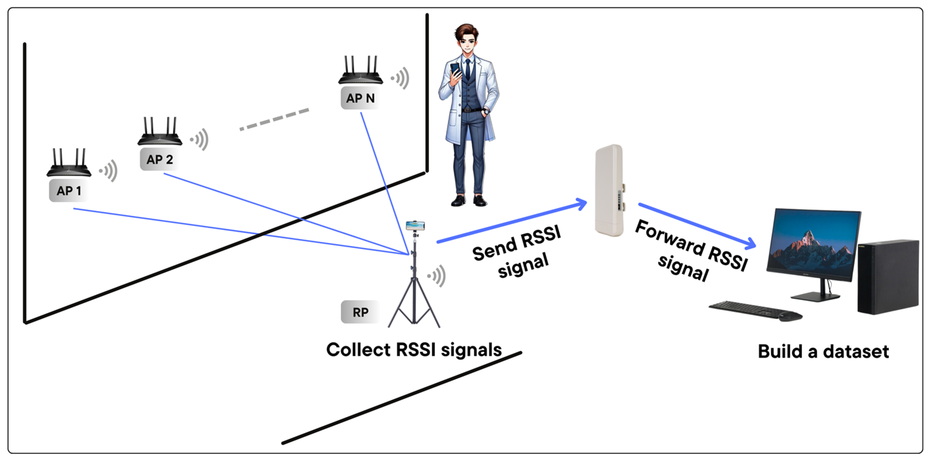
On the software side, a custom-developed mobile application facilitated RSSI data collection and file integration, while a Python script on the server handled the RSSI signal files sent from the smartphone. The overall data collection setup is illustrated in Figure 6. Specifically, the smartphone processed the collected RSSI signals and transmitted them to the server in text file (TXT) format. The files stored the RSSI signal and MAC address in the format REF000000XX, where XX represents the RP number.

The simulation and experimental tests necessitated a significant investment of time. The simulation phase, which spanned approximately 35 days, involved the execution of ten sections, each undergoing 200 epochs. Each epoch took around 25 min, resulting in a total of 84 h per section. Given that the CNN control section was simulated only once, the total time for all sections amounted to approximately 840 h, which was equivalent to 35 days. For the experimental tests, the best-performing section from the simulations was selected for further evaluation. The best-performing model refers to the one that achieved the highest accuracy and lowest loss during simulation processes. This phase included four sections, with signals collected five times at each of the 74 RPs, resulting in 370 data points. The results were analyzed to compute the final average outcome. Each section required 3 h to complete, summing up to 12 h for all experimental tests. In total, the combined time for simulations and experiments amounted to 36 days: 35 days for simulation and 12 h for experimental testing.

To construct the RSSI database, data collection was performed five times at each RP. Each measurement included the timestamp, RSSI values from all visible APs, their corresponding MAC addresses, and associated labels. Data were collected in various orientations (forward and backward) and at different times of the day (morning and afternoon). The procedure was as follows: a smartphone was positioned at a fixed height at each RP and remained stationary during measurements. Data collection spanned six days, with measurements taken in both directions during the morning and afternoon sessions. In total, 22 datasets were collected.

Table 2. Database information and augmentation size.

Database Type	Collection	#of Images
		Before Augmentation	After Augmentation
Training	19 sets	7008	427,488
Test	3 sets	1110	--

provides an overview of the data types, while

Table 3. Types of datasets.

Dataset	Morning Forward	Morning Backward	Afternoon Forward	Afternoon Forward	Number of Data Files
0 m	MF1	MB1, MB2	AF1, AF2	AB1, AB2	7
1 m	MF2, MF3	MB3, MB4	AF3, AF4	AB3, AB4	8
2 m	MF4	MB5, MB6	AF5, AF6	AB5, AB6	7
Number of Data Files	4	6	6	6	22

categorizes the datasets. Morning and afternoon data are denoted as M and A, respectively, while forward and backward directions are indicated as F and B. The numbers represent the collection day. Of the 22 datasets, 19 were used to create the training database, and 3 were reserved for testing. Each data collection session at an RP took approximately 25 s, and the entire measurement process across all 74 RPs required about 40 min, including the time taken to move the smartphone between points. This totaled approximately 15 h over five days.

The fingerprinting technique employed in this study builds on the method proposed by Rashmi et al. [9], with modifications made to the CNN model for improved performance. The process is divided into two phases, as illustrated in Figure 7:

Offline phase:

• RSSI data from all APs are collected at predefined RPs to create a fingerprint database representing the environment. Each RP has a unique fingerprint defined by its location and the RSSI values recorded from nearby APs.
• The collected data are pre-processed and fed into a convolutional neural network (CNN) for simulation training. This process yields a trained model that incorporates the feature information of the RSSI database.

Online phase:

The detailed real-time localization procedure is as follows.

• Real-Time RSSI Data Acquisition: The phone scans nearby WiFi signals and transmits the data to the computer via HPOWD, where the system records the MAC addresses and corresponding RSSI values.
• MAC Address Matching with Database: The system retrieves pre-stored MAC addresses from the database. It aligns the collected MAC addresses with database entries to generate a table. The first row includes the reference MAC addresses from the database, and the second one records the RSSI values corresponding to the matched MAC addresses.
• RSSI Data Transformation to a 16 × 16 Image: After filling in the missing entries, the RSSI values are organized into a 16 × 16 matrix to ensure compliance with the input requirements of the Convolutional Neural Network (CNN) model.
• CNN-Based Localization Prediction: The pre-trained CNN model takes the 16 × 16 RSSI image as input, processes it, and then outputs the predicted location.

To provide a clearer understanding of the transformation process of RSSI signals and the method used to achieve positioning accuracy, the procedure is divided into two phases: the offline phase and the online phase. In the offline phase, RSSI signals are collected and divided into a training set and a test set, both stored as CSV files. These files are then converted into TXT files to extract MAC address lists. The training set undergoes data augmentation to expand the dataset and improve the model’s generalization capability. The augmented training set and the original test set are then used to train a CNN model. This training process produces simulation accuracy, a trained CNN model, and extracted feature information. In the online phase, mobile devices at each RP capture real-time RSSI signals and transmit them to a server via a designated network. The server processes these signals by matching them with the MAC address list and utilizing the feature information obtained during the offline phase. A custom Python script integrates these elements, enabling the system to determine the predicted location. The final output includes the experimental results, which provide the estimated device location based on the most suitable RPs. This two-phase workflow ensures that the system effectively combines preprocessed data and real-time inputs to achieve accurate location predictions.

4.2. Simulation Results

The simulation was conducted using Jupyter Notebook (version 6.5.3) as the software platform, with Python version 3.11.7 (released on 4 December 2023) and TensorFlow version 2.14.0 (released on 27 September 2023). Previous research has established the effectiveness of grouping different techniques across various layers in CNNs. For example, Ren et al. (2017) used the CIFAR-10 and CIFAR-100 datasets and evaluated the performance of different regularization techniques (L1) and normalization methods (BN, LN, and denormalization (DN)) without modifying the network’s layer structure [33]. Ding et al. (2018) compared activation functions in a deep convolutional neural network (DC-NN) based on the MNIST dataset and found that the ReLU function provided the best classification performance [34]. Nanni et al. (2020) demonstrated that varying the type or position of activation functions within the same CNN architecture leads to different outcomes, helping to identify optimal configurations [35]. In their subsequent 2023 study, they further explored the stochastic selection of activation layers [36].

Building on these insights, we conducted a comparative analysis of BN, LN, and LBN, which were applied to the 1st, 2nd, and 3rd layers of a CNN model. To systematically evaluate the contribution of each normalization method, we performed an ablation study, where different normalization techniques (BN, LN, and LBN) were incorporated separately into the CNN model for comparison. The simulation was divided into three parts, each containing an experimental section: CNN + BN (first experimental section), CNN + LN (second experimental section), and CNN + LBN (third experimental section). A separate baseline evaluation using only the CNN model was conducted for comparative purposes. For each experimental section, both the accuracy and loss metrics were evaluated. This approach generated three distinct accuracy values and three corresponding loss values for each part of the simulation. In total, each part of the experiment was characterized by six evaluation components. These results are shown in

Table 4. Classification of the simulation.

	Model Name
Layer 1	CNN	CNN + BN	CNN + LN	CNN + LBN
Layer 2		CNN + BN	CNN + LN	CNN + LBN
Layer 3		CNN + BN	CNN + LN	CNN + LBN

and

Table 5. Results of the simulation.

Accuracy (MAX)	CNN	CNN + BN	CNN + LN	CNN + LBN
Layer 1	0.9054	0.9321	0.9183	0.9469
Layer 2		0.9060	0.9055	0.9180
Layer 3		0.9291	0.9104	0.9365
Loss (MIN)	CNN	CNN + BN	CNN + LN	CNN + LBN
Layer 1	0.2589	0.1898	0.2214	0.1489
Layer 2		0.2530	0.2573	0.2252
Layer 3		0.1943	0.2301	0.1740

. The simulation demonstrated that the CNN model integrated with BN achieved a maximum accuracy of 93.21%. The model incorporating LN reached 91.83%, and the model incorporating LBN achieved a higher accuracy of 94.69%.

In terms of simulation results, among the four models in Layer 1 (Table 5), the CNN + LBN model in Layer 1 (Table 5) exhibited the highest test accuracy and the lowest loss. Initially, the loss values of the CNN + LBN, CNN + LN, CNN + BN, and CNN models were 2.20, 2.27, 3.07, and 2.24, respectively. After 200 epochs of training, these values decreased to 0.14, 0.22, 0.18, and 0.25. The decline in loss indicated the continuous improvement of the models’ performance over the training process. The highest accuracy of each model, used as the benchmark in the final simulation results, was as follows: CNN + LBN reached a maximum accuracy of 94.69% after 195 epochs (loss = 0.14), CNN + LN reached a maximum accuracy of 91.83% after 141 epochs (loss = 0.22), CNN + BN achieved 93.21% after 107 epochs (loss = 0.19), and CNN reached 90.54% after 132 epochs (loss = 0.262). In Layer 2, the CNN + LBN model once again achieved the highest test accuracy and the lowest loss. The initial loss values for the CNN + LBN, CNN + LN, CNN + BN, and CNN models were 3.61, 3.45, 3.21, and 2.24, respectively. After 200 epochs of training, these values decreased significantly to 0.225, 0.257, 0.253, and 0.258. The CNN + LBN model achieved a peak accuracy of 91.8% after 192 epochs (loss = 0.225), CNN + LN reached a peak accuracy of 90.55% after 137 epochs (loss = 0.26), and the CNN + BN model achieved 90.6% after 76 epochs (loss = 0.259), and CNN reached 90.54% after 132 epochs (loss = 0.262). In Layer 3, all models showed a consistent reduction in loss. In Layer 3, the models consistently exhibited a reduction in loss. The initial loss values for the CNN + LBN, CNN + LN, CNN + BN, and CNN models were 2.94, 2.87, 2.94, and 2.24, respectively. After 200 epochs, these values dropped to 0.17, 0.21, 0.19, and 0.25. CNN + LBN achieved a maximum accuracy of 93.65% after 124 epochs (loss = 0.17), CNN + LN reached 91.04% after 153 epochs (loss = 0.23), CNN + BN reached 92.91% after 129 epochs (loss = 0.19), and CNN achieved 90.54% after 132 epochs (loss = 0.262). The results of the ablation study clearly demonstrate that LBN significantly enhances the simulation accuracy of CNN-based indoor positioning systems.

To better understand these results, we present a qualitative analysis below. Although LN has been widely used in RNNs and scenarios characterized by extremely small batch sizes [20], its effectiveness in CNNs might be constrained. Distinct from batch normalization, layer normalization estimates normalization statistics independently for each training case, without using batch-level statistics [20]. As a result, while LN stabilizes training dynamics, it does not explicitly mitigate internal covariate shift, which is one of the key advantages of BN in CNNs. Notably, the CNN + LBN model consistently outperformed other models across all layers. BN normalizes across the batch dimension, while LN normalizes feature channels independently within each sample. Different from them, LBN leverages localized normalization mechanisms, making it more effective for stabilizing feature distributions in WiFi fingerprint-based positioning.

4.3. Principal Component Analysis

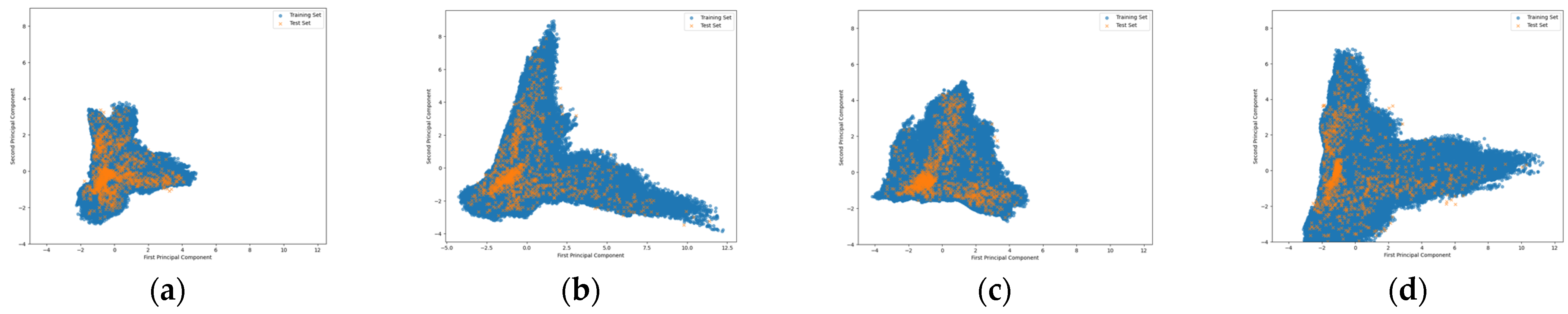
Figure 8 presents the visualization result of principal component analysis (PCA) carried out on both the training and test datasets, spanning four principal components. PCA [9,37,38,39] was employed primarily for visualization, allowing us to analyze the spatial distribution of training and test datasets in a lower-dimensional space. This is instrumental in evaluating how various normalization techniques influence the data representation and, in turn, their potential implications for model generalization. In these plots, blue points represent RPs from the augmented training dataset, while orange points indicate unknown location points from the test dataset. In Figure 8a, which depicts the data distribution without the application of BN, LN, or LBN, there is significant overlap between the training data (blue) and test data (orange). This overlap highlights a high risk of overfitting, as the training and test datasets are not sufficiently distinct. Moreover, the test data are heavily concentrated in the center, which could negatively affect the model’s ability to generalize to unseen data. In Figure 8b, after applying batch normalization (BN), the test data distribution becomes more dispersed, and the training data effectively span the test dataset. This broader spread reduces the risk of overfitting and improves alignment between the training and test sets. The training dataset also exhibits a more structured representation, improving clarity in the PCA transformation space. In Figure 8c, where layer normalization (LN) is applied, the data distribution improves compared to (a), with less overlap between the training and test datasets. However, the separation is not as effective as that in (b) (BN). This indicates that while LN contributes to improving generalization, its ability to mitigate overfitting is not as potent as that of BN. The test data show a more natural spread than (a), yet it does not cover as extensive a region as in (d) (LBN). In Figure 8d, which illustrates the distribution after applying localized batch normalization (LBN), the training dataset is evenly dispersed over a wider region in the PCA transformation space. This dispersion suggests that the model has reduced the risk of becoming trapped in local optima during training. The test dataset also demonstrates a more natural distribution, indicating improved generalization performance compared to BN (b) and LN (c).

4.4. Experimental Results

This section evaluates four methods for the CNN-based positioning system: Method 1 employs the original CNN model, Method 2 integrates BN into the CNN model, Method 3 integrates LN into the CNN model, and Method 4 incorporates LBN into the CNN model. The performance of these methods was validated through online experiments. During testing, a mobile device captured real-time RSSI information, including MAC addresses, from various APs at different RPs. These data were transmitted to a positioning server, where it was processed by a classifier model to predict the device’s position. The experimental setup involved moving the mobile device to each RP within a predefined environment (from RP1 to RP74) and collecting data five times at each RP. The classifier model on the server analyzed the collected data to calculate localization accuracy. The interval between consecutive RPs in this study is 2 m, resulting in a positioning precision of 4 m. To evaluate simulation outcomes, three different margins (0, 1, and 2) were applied. A margin of 0 indicates that the decision made at a specific RP is completely accurate. A margin of 1 means the positioning decision falls within the range of RP − 1 to RP + 1, while a margin of 2 implies the decision lies within RP − 2 to RP + 2. Since the database contains 74 RPs and n tests were conducted at each RP, the total number of samples is a multiple of 74. The accuracy probability is calculated using the following formula [9]:

$$Probability of accuracy [\%]={\displaystyle \frac{success count}{total samples}}\times 100$$

(12)

The online test results are summarized in

Table 6. Localization accuracy across margins.

	Accuracy (%) (0 RP Margin)	Accuracy (%) (1 RP Margin)	Accuracy (%) (2 RP Margin)
CNN + LBN	39.46	78.11	92.97
CNN + LN	34.59	74.32	89.73
CNN + BN	34.86	77.84	91.89
CNN	33.51	71.08	87.84

. The real-time localization accuracy of the CNN model was 87.84%, slightly lower than its simulated accuracy of 90.54% (Table 5). Similarly, the CNN + BN model achieved a real-time accuracy of 91.89%, which is lower than its simulated result of 93.21%. The CNN + LN model achieved a real-time accuracy of 89.73%, which is lower than its simulated result of 91.83%. The CNN + LBN model recorded the highest real-time accuracy of 92.97%, though it still fell short of its simulated performance of 94.69%.

In the WiFi fingerprint-based indoor positioning experiment using RSSI signals, additional error metrics were calculated for all models in

Table 7. Comparison of mean error, variance, and standard deviation across CNN, CNN + BN, CNN + LN, and CNN + LBN models for WiFi fingerprint-based positioning.

	Mean (m)	Variation	Standard Deviation
CNN + LBN	1.27	3.97	1.99
CNN + LN	2.07	7.61	2.75
CNN + BN	1.48	4.3	2.07
CNN	2.21	12	3.46

. The CNN model showed a mean error of 2.21 m, a variance of 12 m², and a standard deviation of 3.46 m. By incorporating BN, the CNN + BN model significantly improved these results. It achieved a mean error of 1.48 m, reducing the error by 0.73 m. Its variance was reduced to 4.3 m² (a decrease of 7.7 m²), and the standard deviation dropped to 2.07 m (a reduction of 1.39 m). After the integration of LN, the model exhibited a mean error of 2.07 m, a variance of 7.61 m², and a standard deviation of 2.75 m. While LN improved the variance and standard deviation compared to the baseline CNN model, it was less effective than BN in reducing the mean error. The CNN + LBN model demonstrated even greater improvements over both the CNN and CNN + BN models. It achieved a mean error of 1.27 m, reducing the error by 0.94 m compared to the CNN model. Its variance decreased to 3.97 m², an improvement of 8.03 m², while the standard deviation was reduced to 1.99 m, representing a decrease of 1.47 m. These results clearly indicate that the LBN approach is more effective than BN in processing RSSI data for fingerprint-based positioning systems.

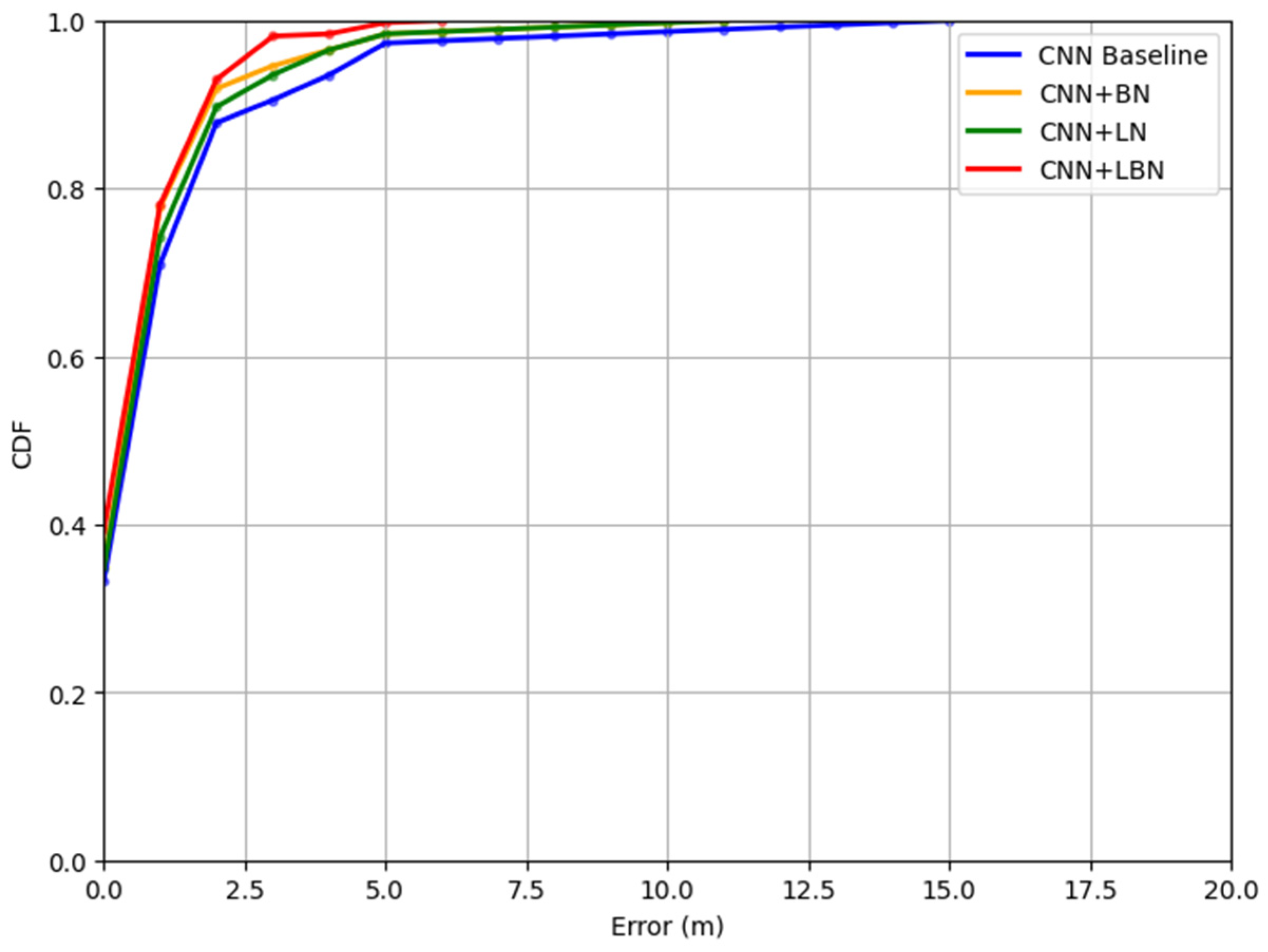
The positioning accuracy of the proposed LBN was further assessed using the cumulative distribution function (CDF) of location error within a specified distance, as illustrated in Figure 9. When comparing the performance of the CNN baseline (represented by the blue line), CNN + BN (the yellow line), CNN + LN (the green line), and CNN + LBN (the red line), it is evident that all four methods achieve a probability exceeding 85% within a 2-m error range. Across the entire error range, CNN + LBN consistently outperforms the CNN baseline, demonstrating its superior localization accuracy. Furthermore, the results indicate that for a 1-m error threshold, CNN + LBN achieves a CDF value of 78%, whereas CNN baseline only reaches 71%. This significant difference highlights the enhanced positioning accuracy brought about by LBN.

5. Conclusions

This study presented a CNN model enhanced with LBN to improve the performance of RSSI-based indoor fingerprint positioning systems. Through extensive simulations and real-time experiments, the effectiveness of BN, LN, and LBN in enhancing model accuracy was validated. The proposed CNN + LBN model consistently outperformed the baseline CNN, CNN + BN, and CNN + LN models in real-time positioning tasks, achieving a real-time accuracy of 92.97%. This marked a significant improvement over the traditional CNN approach. While real-time accuracies for all models were slightly lower than their simulation results, the CNN + LBN model demonstrated the most robust performance across both scenarios. These findings underscore the potential of LBN in enhancing the generalization and precision of CNN-based indoor positioning systems, particularly in real-time applications. Future research should focus on further improving the model by utilizing larger and more diverse datasets and exploring additional normalization techniques. Such advancements could help address the residual performance gap between simulation and real-time results, further strengthening the model’s reliability and scalability for practical deployment.