Article

Electronic Artificial Intelligence–Digital Twin Model for Optimizing Electroencephalogram Signal Detection

by
Alessandro Massaro
Department of Engineering, LUM-Libera Università Mediterranea “Giuseppe Degennaro”, S.S. 100-Km.18, Parco il Baricentro, 70010 Bari, Italy
Electronics 2025, 14(6), 1122; https://doi.org/10.3390/electronics14061122
Submission received: 11 February 2025 / Revised: 6 March 2025 / Accepted: 10 March 2025 / Published: 12 March 2025
(This article belongs to the Special Issue Emerging Biomedical Electronics)

Abstract

:
The study is focused on the application of the electronic proof of concept Digital Twin (DT) model supporting Electroencephalogram (EEG) signal detection and interpretation. The EEG DT model integrates two open source tools: a first tool used for the circuit modeling and simulation of the electrodes, and a second one implementing an Artificial Intelligence (AI)-supervised algorithm to classify and adjust a noisy EEG signal. Specifically, the DT model adopts the Random Forest (RF) AI-supervised algorithm, replacing the signal filtering process and facilitating the time–domain peak and the wave shape morphology reading of a noisy detection. In order to prove the DT’s efficacy, the RF model is trained by considering the specific case of detections of EEG of patients under the effects of alcohol. The choice of the RF algorithm is justified by its good performance parameters. For the specific dataset, the RF exhibits a probabilistic error slightly lower than that of the ANN and a better cleaning action. The goal of the paper is to provide a methodology to use ‘intelligent’ electrodes supporting EEG data processing during data acquisition and to optimize the measurement’s interpretation through a data post-processing process. The proposed EEG DT could represent an alternative to the traditional denoising signal processing approaches.

1. Introduction

Circuit modeling and simulation are fundamental to understanding and interpreting biomedical signals, such as Electroencephalograms (EEGs) and Electrocardiograms (ECGs) [1,2,3,4,5,6,7,8]. Studies about EEG signals have focused their attention on the need to suppress white noise and spikes to facilitate diagram reading [9,10,11,12,13]. Other studies evaluate the possibility of using machine learning for the denoising process [14] and to interpret brain disorders [15]. Digital Twin (DT) models processing EEG signals are adopted for noise filtering and defalsification processes [16] that are used, for example, to simulate the administration of a drug that influences the whole brain [17] or for rehabilitation procedures [18]. The study of the EEG is based on the morphological characterization of EEG signal processing by separating the background from the signal, detecting voltage information spikes, and reading waveform amplitude shapes and durations [19]. Specifically, the analysis of the time–domain’s EEG signal trend is useful for the diagnosis of epilepsy [20] and Parkinson’s disease [21], the study of stimulation therapy, and the detection of other pathologies [22,23]. EEG signal trends are classified into five main categories (delta (0.5–4 Hz), theta (4–8 Hz), alpha (8–13 Hz), beta (13–30 Hz), and gamma (>30 Hz) [24]), carrying information about mental stress [25]. Focusing the attention on alcoholic EEG signals [26,27,28], some studies highlight the possibility to distinguish, by means of peak analysis, the alcoholic cases from the non-alcoholic ones [28]. The goal of the proposed paper is to fix a specific case of study for alcoholic EGG signals in order to structure an AI-based DT model to replace the common process of signal filtering and facilitate the time–domain peak and wave shape morphology detection for noisy measurements. This proof of concept is better sketched in Figure 1; the proposed DT model is composed of a circuit model reproducing the EEG signal reading procedure of a couple of electrodes and an AI-supervised algorithm able to adjust a noisy signal disturbed by Flicker and white noises, which are typical of EEG detection systems [3,29] and act at the input of the amplification systems. The scheme of Figure 1 follows a bipolar configuration; both electrodes are placed on active sites of the area of interest, and the detected signal corresponds to the difference that emerges between the activities of the two sites. In addition to the two inputs, an amplifier also requires a ground connection, which allows the current to flow between it and the active or reference conductor, thus allowing the amplifier to operate (see Figure 1). The Flicker and white noises are coupled into the amplification system, providing a noisy signal, which will be classified and cleaned by the AI engine. Specifically, the paper proposes the implementation of a DT able to define an AI-based methodology to correct and clean disturbed alcoholic EEG signals by means of training of the Random Forest (RF) algorithm, which is suitable for complex DT models characterized by different noise sources [30]. The circuit model of Figure 1 takes into account the equivalent circuit cascade of the electrical elements, such as the equivalent resistances and capacitances of the skin, skin/electrode interfaces, and electrodes [3,5].
The goal of the paper is to propose an alternative denoising solution adaptable to different technologies based on AI classification concepts. The model is simulated by combining the circuit simulation with AI data processing, proving the cleaning of a noisy signal. Two AI-supervised algorithms are considered for data processing: an Artificial Neural Network (ANN) and Random Forest (RF). In order to optimize the training model, it requires a fixed pathology, such as alcoholism.
The paper is structured as follows.
-
Materials and Methods (Section 2): a discussion of the open source tools used for the implementation of the model in Figure 1 and of the electrical/electronic parameters describing the noisy environment characterizing EEG signal detection;
-
Results (Section 3): a discussion of the circuit simulations and the AI results by analyzing the algorithm performances and demonstrating the functioning of the DT ‘proof of concept’;
-
Discussion (Section 4): an explanation from the perspectives of DT implementation, including advantages, bottlenecks, limits, statistical analysis, and perspectives;
-
Conclusions (Section 5): a summary of the DT results.

2. Materials and Methods

The materials and methods are mainly focused on aspects concerning the problem of EEG signal detection due to the presence of noise, circuit modeling, and the AI engine supporting the reading of the noisy signal. All data are processed by using a Intel Core i5 2.4 GHz/16 GB RAM processor.

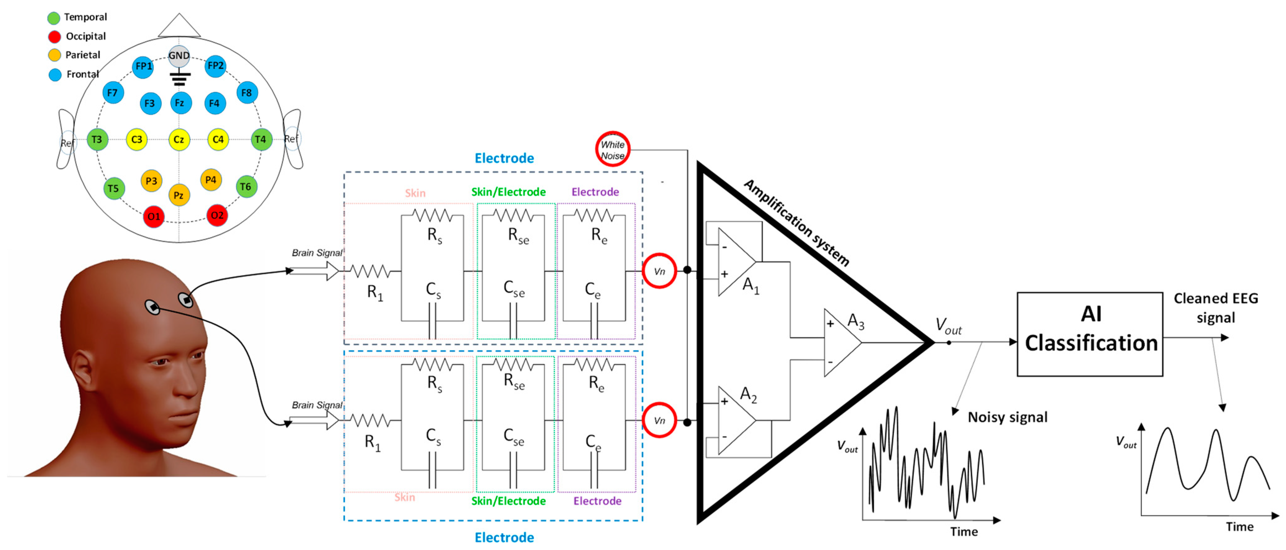
2.1. Electrodes and Related Electronic Noise

EEG signal detection is typically performed by means of contact and non-contact dry electrodes. The names of the electrode sites are alphabetical abbreviations identifying the lobe or area of the brain transmitting a time voltage signal:
  • F = frontal
  • Fp = frontopolar
  • T = temporal
  • C = central
  • P = parietal
  • O = occipital
Different electronic noises could change the EEG morphology for wet and dry electrodes. Dry electrodes are more inclined to noise due to their weak contact increasing the equivalent impedance of the skin/electrode interface. Other possible important artifacts are thermal white noise (also called Johnson–Nyquist noise), flicker noise, line noise, and the half-cell effect at the skin-to-electrode interface [31,32]. Thermal and Ficker noise are the most common noise sources influencing mainly electrodes’ amplifiers. The thermal or white noise is characterized by the following power density:
v w n 2 = 4 K B T B R ,
where vn is the noise voltage expressed in Volts rms units, indicating a measured value obtained driving a totally noise-free bandpass filter (with bandwidth B) with a voltage generated by a resistor at temperature T (absolute temperature expressed in Kelvin units); the KB parameter indicates Boltzmann’s constant (Joules per Kelvin); R is the resistor’s value (Ohms); and B = ∆f is the band. The Flicker noise (pink noise) [33] is prevalent at lower frequencies with a 1/f power spectral density (it is opposed to thermal and shot noise, which have a “white” spectrum). The spectral density of the Flicker noise is given by
v f n 2 = 1 f a
where f is the frequency and 0 < a < 2, with exponent α usually close to 1. One-dimensional signals with a = 1 are usually called pink noise.

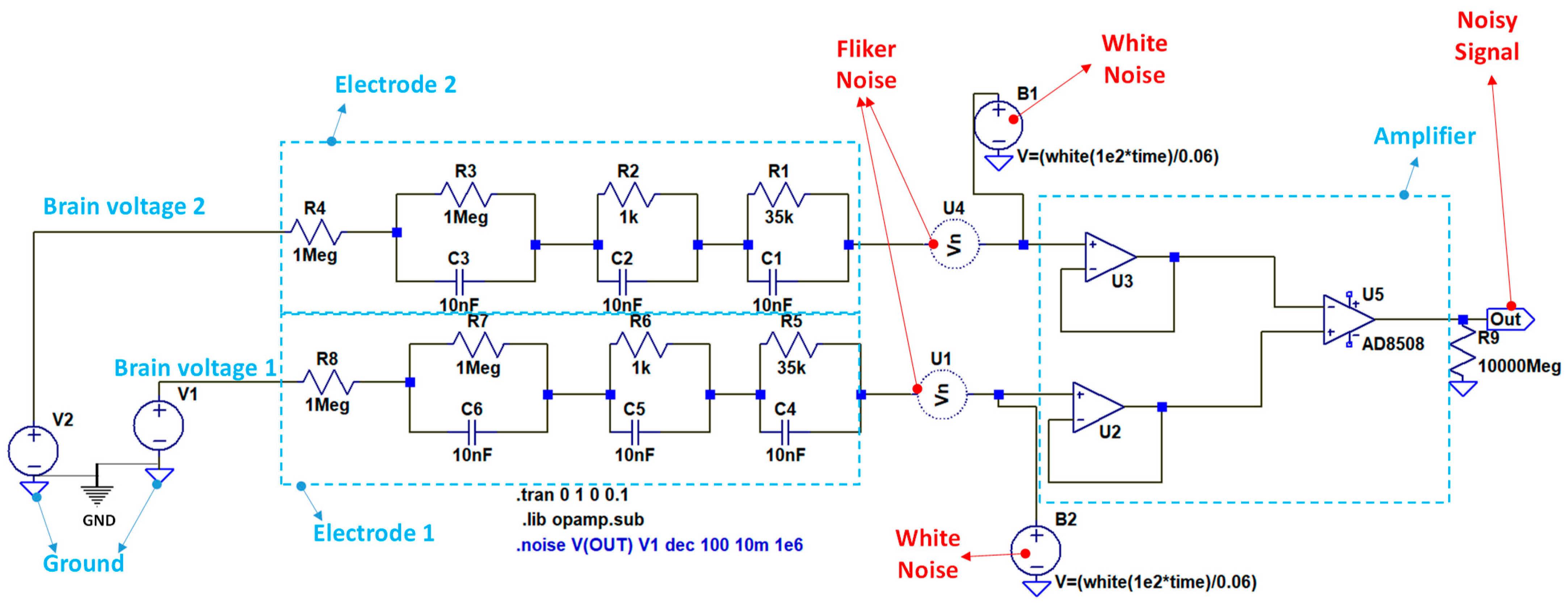
2.2. Circuit Modeling and Simulation

The circuit model of the Figure 2 is implemented using the LTSpice open source tool [34] (version 24.1.0), which is a free ‘SPICE’ simulator engine with a graphical schematic capture interface producing simulation results. The LTSpice circuit model used to simulate noisy conditions changing the EEG signal is illustrated in Figure 2. The circuit model of Figure 2 reproduces the real behavior of the EEG electrode measuring a brain signal.
As sketched in Figure 1, the simplified EEG electrode system is modeled electrically, with four stages of equivalent impedance; the first three are related to the skin, the skin/electrode interface, and the electrodes, respectively, and the last one is the amplification system. The electrical parameters characterizing the circuit model are the following (see Figure 1):
-
Skin stage: resistance of the subcutaneous layer R1 (R4 and R8 of Figure 2), resistance of the stratum carenum RS (R2 and R7 of Figure 2), and capacitance of the stratum carenum CS (C3 and C6 of Figure 2); Rs is in the series parallel to CS and RS.
-
Skin/electrode stage (parameter modeling the global effect of gel, sweat, moisture, and hair impedance): equivalent resistance RSe (R2 and R6 of Figure 2) and equivalent capacitance CSe (C2 and C5 of Figure 2); Rse is parallel to CSs.
-
Electrode stage: equivalent resistance Re (R1 and R5 of Figure 2) and equivalent capacitance Ce (C1 and C4 of Figure 2); Re is parallel to Cs.
-
Amplifier stage: it is composed of three operational amplifiers (A1 and A2 are in a non-inverting configuration and are connected with the A3 amplifier).
At the input of the amplification stages are coupled the Flicker and white noises according to the connection scheme of Figure 2. Both of the noises are modeled in the LTSpice framework by voltage generators implementing Equations (1) and (2). Specifically, the white noise (default LTSpice function) signal is implemented by the voltage generators B1 and B2 (voltage sources with an inner resistance of 0 Ohm, modeling the white noise), and the Flicker noise is implemented by means of specific LTSpice libraries [35] integrated in the U1 and U4 generators of Figure 2. The noise model hypothesizes the operation of embedded Flicker voltage noise sources (connected in series [35]) and the white noise superimposed (generators B1 and B2) to both the electrodes following in-line coupling [30]. The input of the whole circuit model (V2 voltage generator of Figure 2) is an EEG brain signal found in the open dataset [36] and related EGG correlations with alcoholism. The testing of the proposed circuit model is focused on the features of the alcoholic EEG signals because the AI engine is trained by this data typology. The electrical parameters of the circuit simulation are listed in Table 1.
The input brain signal of the circuit in Figure 2 is loaded into the circuit by means of the Piecewise Linear (PWL) option, enabling the importing of an external text file into the local repository.

2.3. AI Brain Signal Classification

AI classification is performed by using the open source Konstanz Information Miner (KNIME) tool [37]. The KNIME workflow is designed to pre-process, process, and extract the classification results (see Appendix A). The input dataset [35] is imported into the local repository and merged into a unique table neglecting the time attribute (only a progressive time attribute is considered for data processing, avoiding redundancies). The workflow implements two AI-supervised algorithm: the RF and the ANN adopted for a performance comparison. Concerning the RF approach, each decision tree model is built and split within a chosen tree, which is initially random, and the predicted value for a leaf node is characterized by minimal variance (target value). An example of a tree model is discussed in Appendix A.
Data are also normalized (from a value of 0 to 1) to facilitate the interpretation of results.
The optimized hyper-parameters obtaining the best algorithm performance are the following:
RF algorithm single EEG input signal: 100 tree models (number of trees to be learned); tree depth = 10 (limit number of levels); minimum node size = 5 (minimum number of records in child nodes); training dataset 80%; testing dataset 20%; linear sampling approach for the construction of the testing dataset;
RF algorithm double EEG input signals: 250 tree models; tree depth = 10; minimum node size = 5; linear sampling approach for the construction of the testing dataset;
ANN algorithm single EEG signal: 100 as the maximum number of iterations; 1 hidden layer; 10 neurons for the hidden layer; training dataset 80%; testing dataset 20%; linear sampling approach for the construction of the testing dataset;
ANN algorithm double EEG input signals: 400 as the maximum number of iterations; 5 hidden layers; 25 neurons for the hidden layer; linear sampling approach for the construction of the testing dataset.
The best algorithm performances are achieved by performing a key-fold cross-validation analysis using 10 folds. The training dataset is constructed by considering selected cases of alcoholic EEG signals; a first training model is obtained by considering signals of the same alphabetical identification (F, Fp, T, C, P, O, A) of different patients with ‘alcoholic’ characteristics, and a second training model is constructed by considering a unique patient with signals detected in different positions of the electrode. The total number of records of the training model is 1792. The estimated performance parameters of the supervised algorithms are the coefficient of determination R2, the Mean Absolute Error (MAE), the Mean Squared Error (MSE), the Mean Signed Difference (MSD), and the Root Mean Squared Error (RMSE) [38].

3. Results

The results follows the data processing scheme of Figure 2 and are related to the EEG DT circuit simulation integrating the noise signals and, successively, the AI results processing the output of the circuit model.

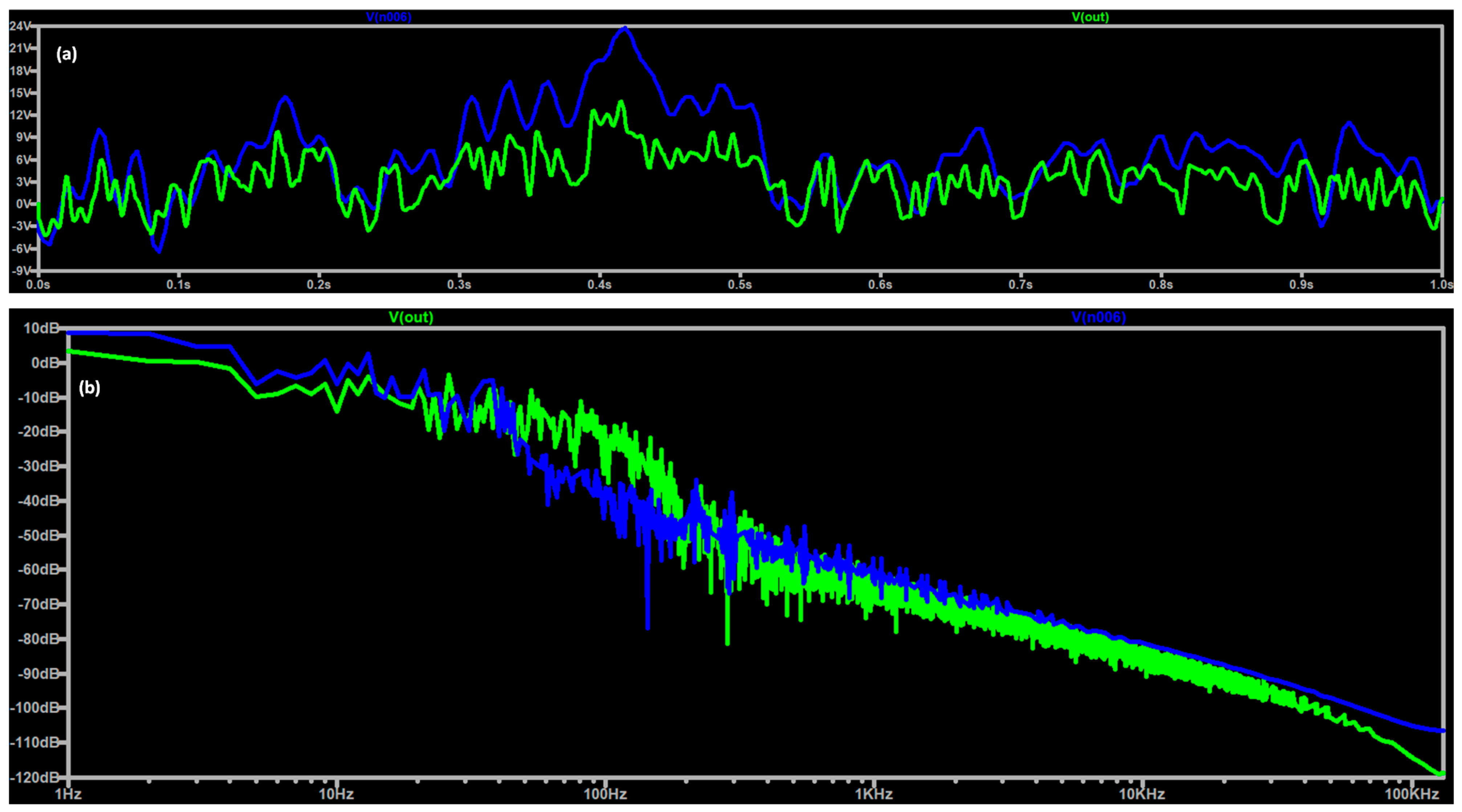
3.1. Noise Modeling and EEG DT Circuit Simulation

The Flicker noise is simulated by analyzing the frequency response of the U2 and U3 operational amplifier. Figure 3 proves the 1/f trend of the frequency behavior due to the application of the Flicker noise sources (U1 and U4) at the input of the operational amplifiers.
The effect of both the Flicker and the white noises is observed in Figure 4a,b. The time –domain brain signal of the EEG alcoholic trend is considerably modified by the combined effect of the noise sources, providing a large number of ripples at the output of the electrode and generating confusion in the interpretation of the peak trend by not allowing for the distinction between alcoholic and non-alcoholic EEG, as discussed in [28]. Furthermore, the noise effect is also observed in the frequency domain in a large band. The simulated noisy output signals are considered for testing of AI classification. Figure 5a,b illustrates the EEG voltage trends detected by a couple of electrodes and the output noisy signal.

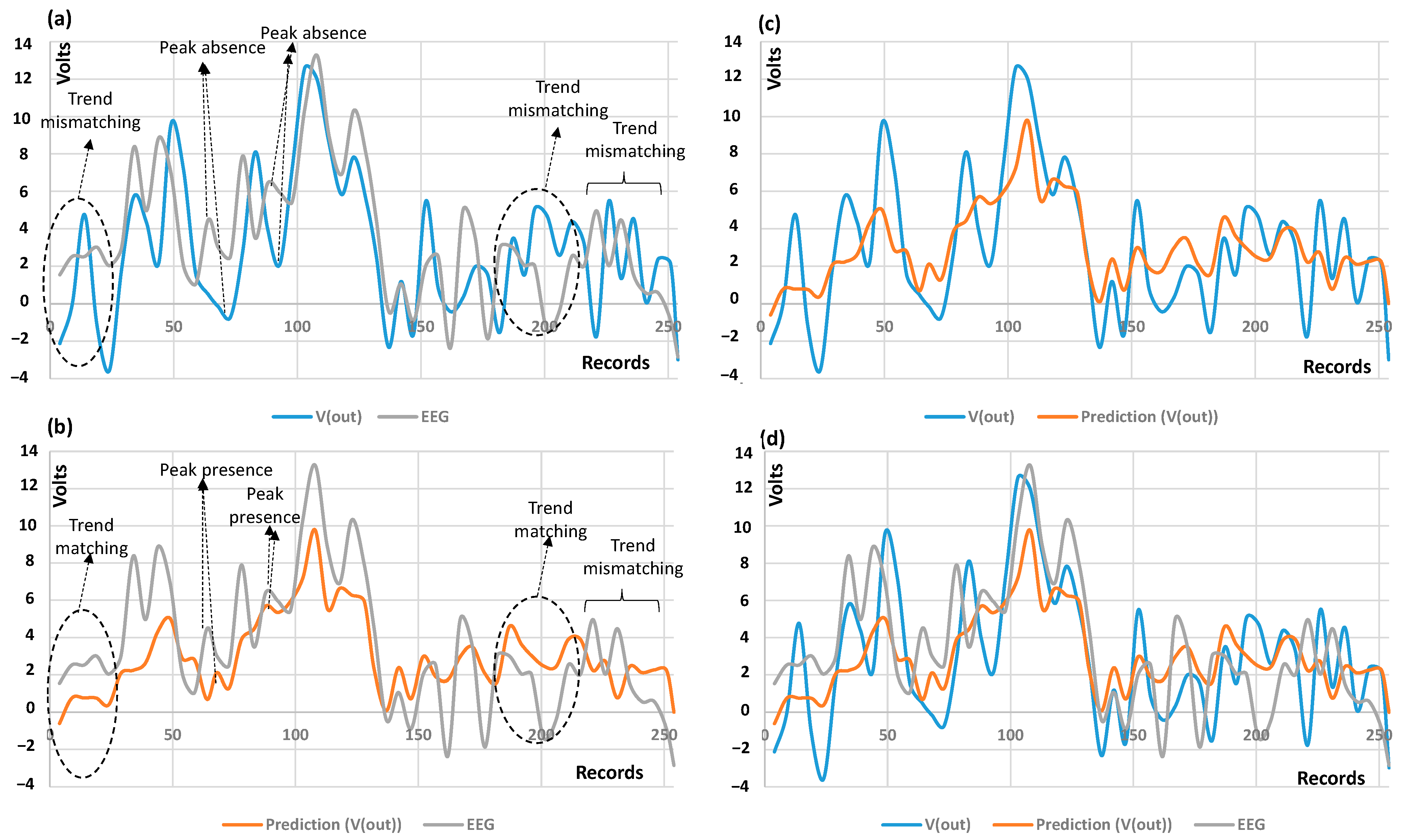
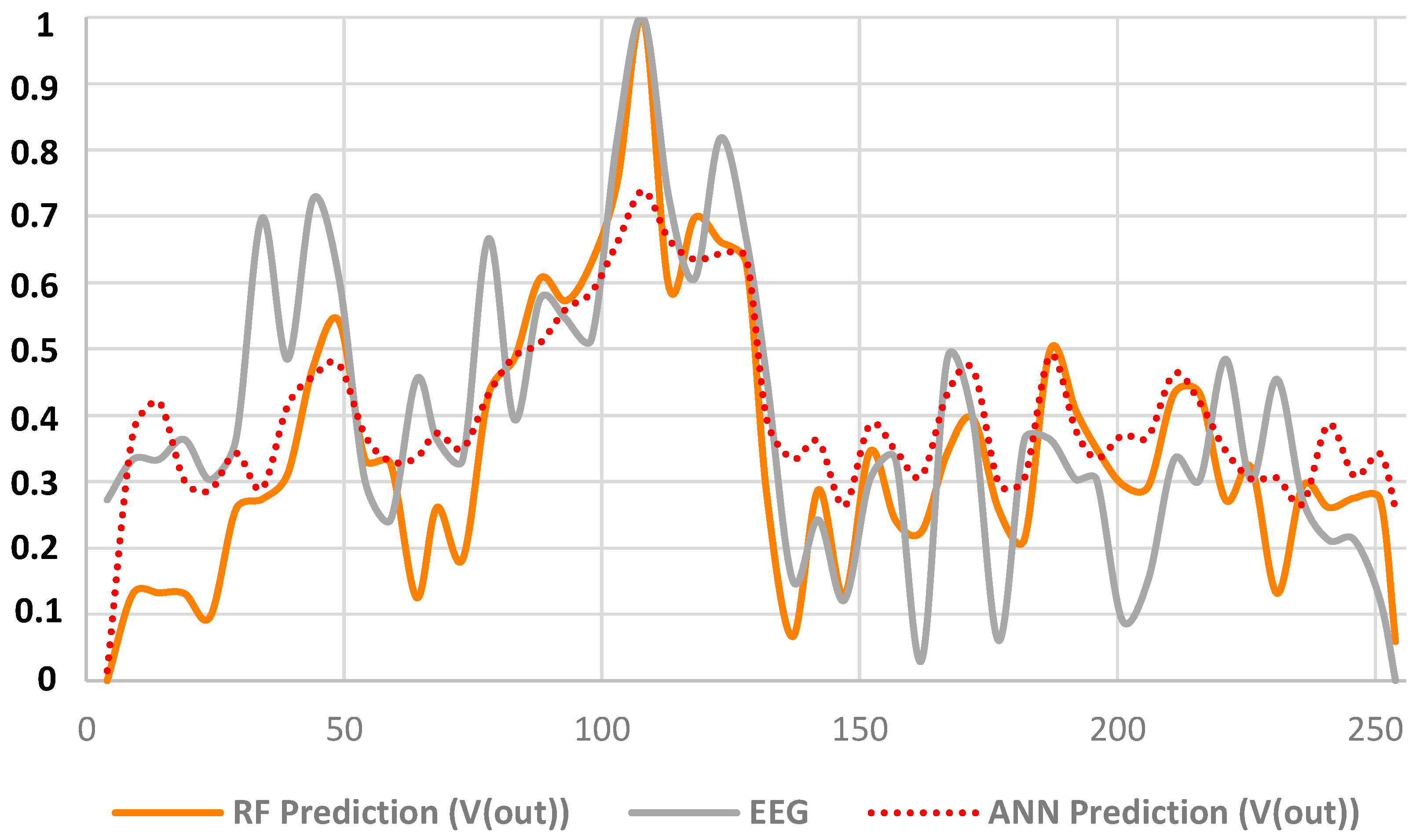
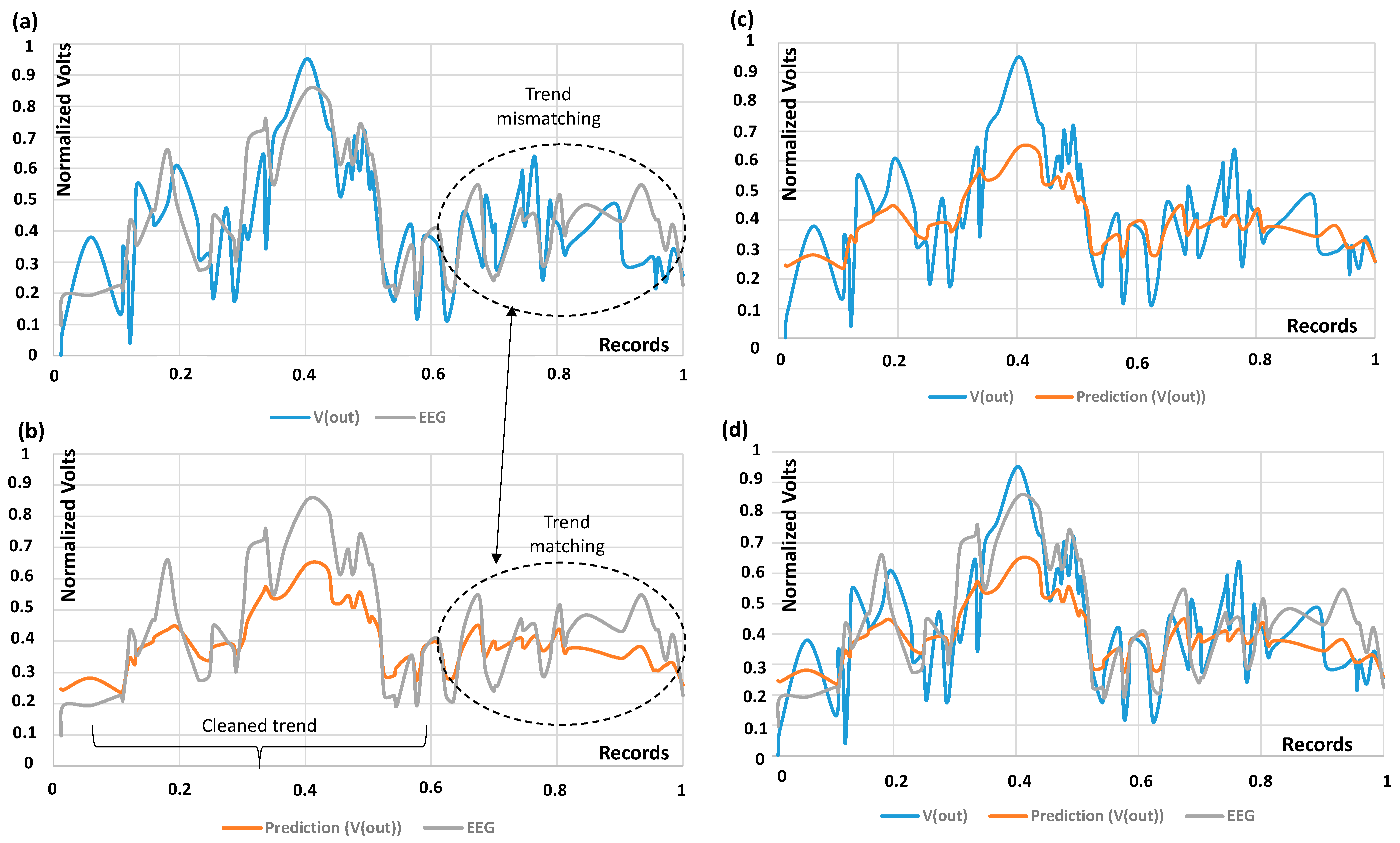
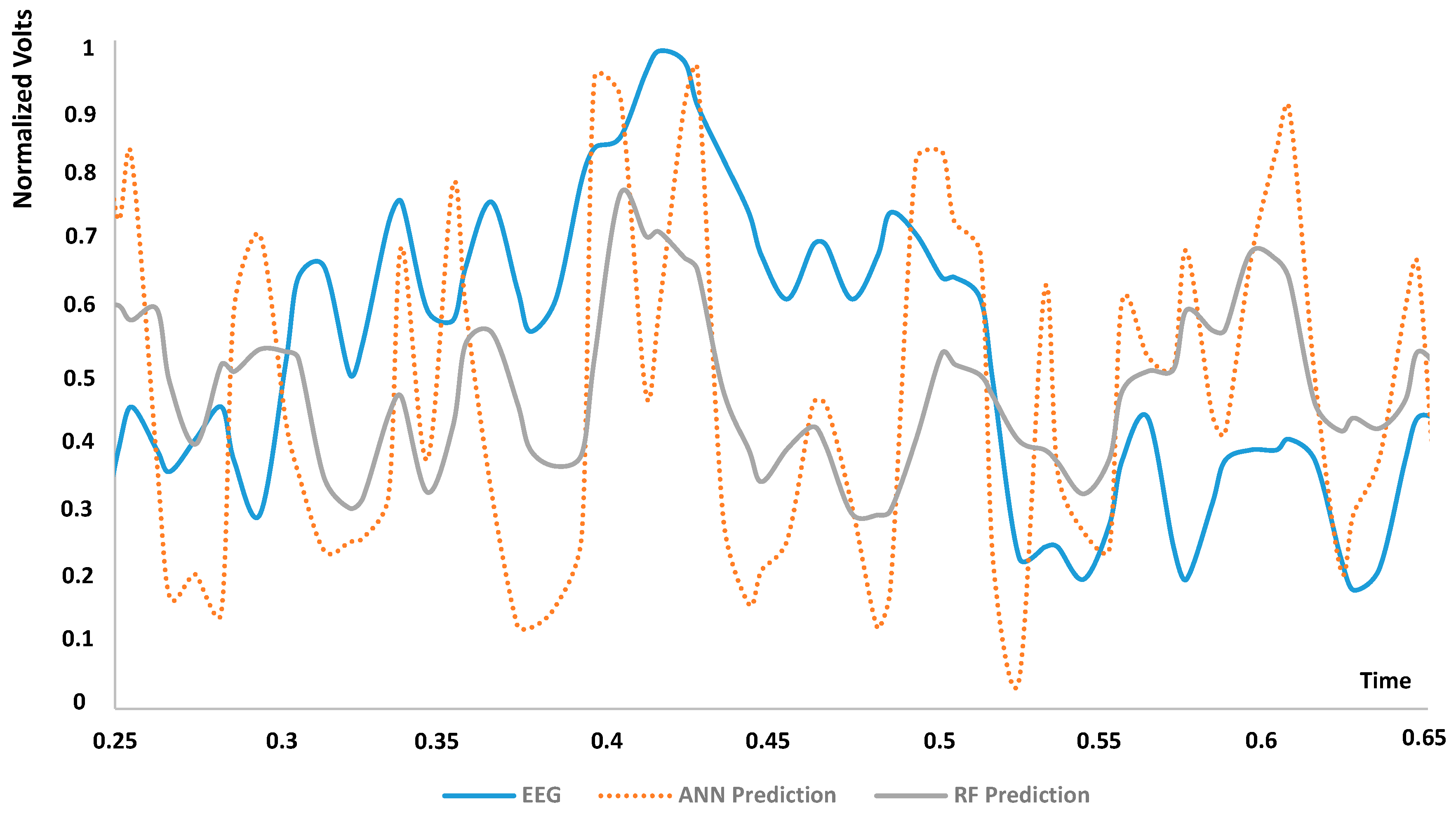
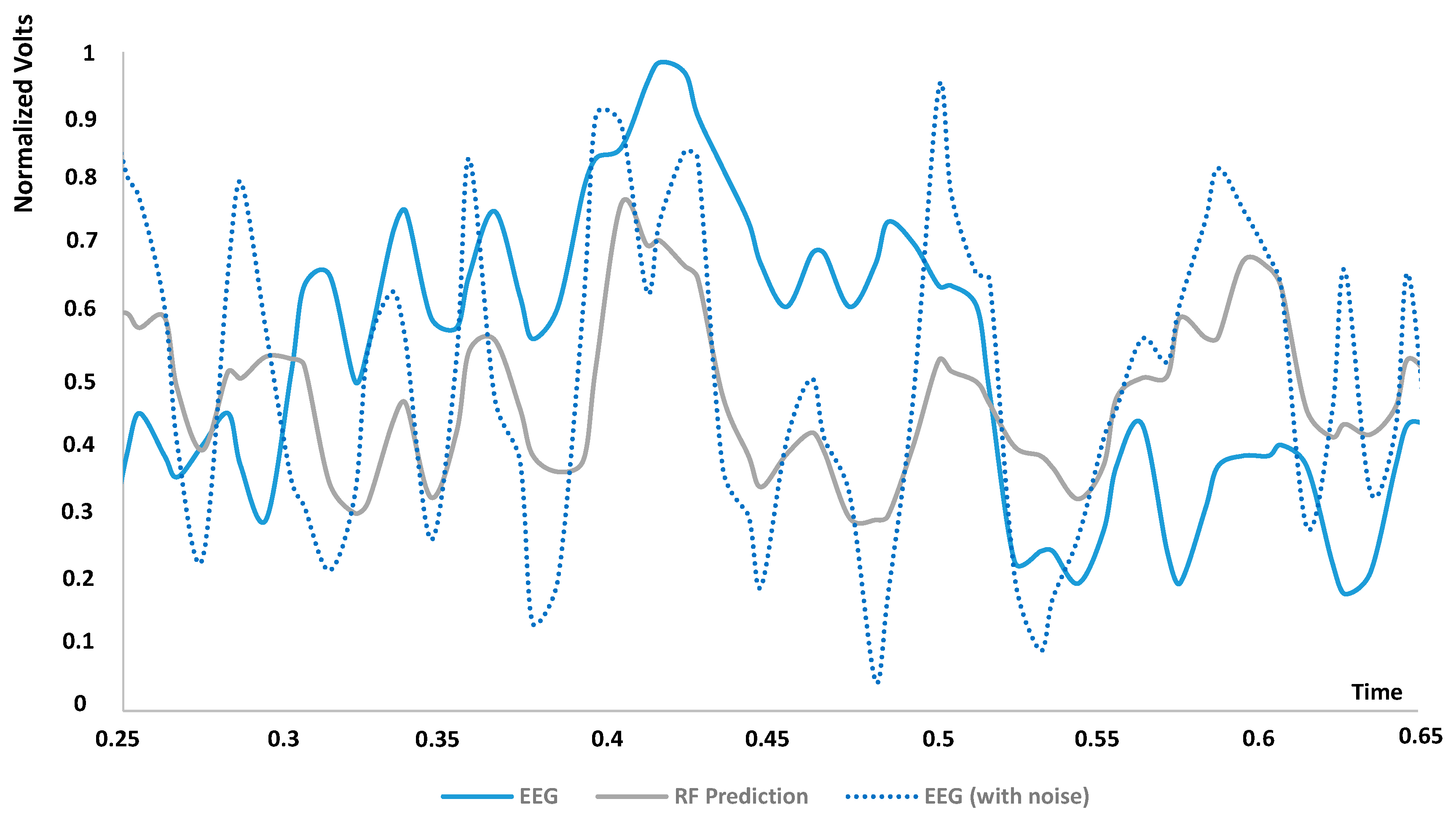
3.2. AI Results: RF and ANN Prediction and Performances

The goal of the proposed DT model is to adopt AI classification to prove the possibility of reconstructing the original brain signal. As a first check for signal reconstruction, the same EEG brain voltage coupled to both of the electrodes in Figure 2 is considered. The results of Figure 6a–c highlight the effect of the noises when the signal trend is mismatching and in the presence/absence of peak artifacts between the noisy simulated signal and the EEG original signal. The diagram in Figure 6a shows that the noise greatly distorts the real EEG signal, confusing the relative reading. We observe that the plots of Figure 6 refer to a single patient with a training model performed by the signal detected in different brain parts (classified by alphabetical identifications). The results of Figure 6 prove that the peak trend of the predicted signal is close to the trend of the original EEG alcoholic signal.
In order to better compare the predicted trend versus the original one, the results are normalized to the unit value (Figure 7 shows the normalized results of Figure 6b), making clear the matching between the original and the reconstructed RF signal (the predicted signal) and, furthermore, decreasing the error rate. Figure 7 proves that the RF signal is closer to the EEG signal compared with the ANN one.
In Table 2 are listed the statistical performance parameters of the optimized RF and ANN algorithms; the comparison shows the better performance of the RF algorithm.
A k-fold cross-validation algorithm is further performed to check the RF and the ANN algorithm performances. In Table 3 are indicated the MSE values for both of the algorithms using 10 as the number of validation tests (k = 10). Also, in this case, a better performance of the RF algorithm is observed.
The training model is successively constructed by considering different patients considering EEG signals of the same brain part classified by the same alphabetical identifications. Also, in this case, as proven by Figure 8a–d, the peak trend of the predicted signal is very close to the trend of the original EEG alcoholic signal, although it is observed that that the noises greatly distort the real EEG signal (V(out)), confusing the relative reading (see Figure 8a).
For the second check for signal reconstruction are considered two EEG brain voltages related to an Fp configuration, each one coupled with an electrode, as in Figure 2. As observed in Figure 9, the RF prediction with a fully noisy condition is closer to the original EEG signal if compared with the ANN prediction; due to the wavier behavior, ANN seems to be more sensitive to noise. In order to highlight the ‘cleaning’ function of the RF attenuating the ripple amplitude due to whole noise effect, in Figure 10 is shown the comparison between the clean EEG signal, the RF-predicted voltage for a noisy condition, and the output voltage simulated for a noisy condition. Concerning the computational cost of the numerical results found in this paper, a few seconds are enough to execute both the circuit simulator and the AI kernel.

4. Discussion

4.1. Advantages, Disadvantages, Limits, Perspectives, and Innovative Aspects of the EEG DT Model

The proposed DT model comprises the merging of different application tools and methodologies, including circuit simulation and AI data processing. In Table 4 are listed the main advantages and disadvantages of the proposed methodologies.
Limitations of the proposed model are mainly in the use of different tools applied to an open dataset [35]. In real scenarios, the tools should be integrated into a unique platform and applied to new measurements, which will determine specific sampling and parameter/hyper-parameter settings. Furthermore, a comparison between predicted results with the EEG ones is necessary. This comparison will support output interpretation regarding the presence or the absence of peaks and possible matching or mismatching of the voltage morphology. The main benefits are the customization of the whole EEG detection system by fixing data sampling and the automatization of data interpretation by means the comparison between real data and imulation ones. In Table 5 are discussed these aspects.
The main innovative aspects discussed in the proposed paper are the following:
  • A DT integrating a circuit simulator processing a real EEG signal to test the setting of the EEG DT to optimize the adjusting process;
  • A DT able to select the most suitable AI algorithm using workflow implementation by checking the algorithm’s performance (rapid check of the performance and the possibility to use the same data pre-processing method to execute different AI algorithms in little time);
  • A DT with configurable physical and physiological parameters (impedances of skin, gel, sweat, moisture, and hair);
  • A DT usable for a real-time check of the detected EEG signal;
  • A DT that is potentially usable for different EEG pathologies to construct a specific EEG training dataset to be processed by the AI-supervised algorithms.

4.2. EEG Hardware and Software Solutions

The proposed EEG DT model is to be integrated into existing EEG systems. Commercial hardware devices are characterized by different resolutions (12 bit, 14 bit, 24 bit), sample rates (125 Hz, 128 Hz, 200 Hz, 250 Hz, 256 Hz, 512 Hz), and numbers of channels (1, 4, 5, 8, 14, 16) [39]. Different physical characteristics characterize the electrodes, such as mechanical stiffness and flexibility [40]. Concerning these features, the DT must be adapted to the measurement procedure and the sampling approach to be compatible with the specific hardware system. The software is typically supplied with the hardware to adjust and avoid EEG disturbances. In this direction are adopted common pre-processing pipelines, such as Independent Component Analysis (ICA) [41,42], Canonical Correlation Analysis (CCA) [42], Artifact Subspace Reconstruction (ASR) [43], wavelet denoising [44], bandpass filtering, and Finite Impulse Response (FIR) filtering [45]. The proposed DT signal processing method is a candidate as an alternative to the listed methodologies.

4.3. Bland–Altman Performance and MSE Metrics for ANN and RF Benchmark Comparison

The basic statistical error metric of Table 2 and the k-fold cross-validation test of Table 3 prove the good performance of the ANN and RF algorithms. Other techniques are proposed in the literature to provide further information about the deviation between the measured and processed values. A more commonly used technique is the Bland–Altman approach [45,46,47,48,49], which is used to analyze the agreement of two different measurement methods. In the proposed work, the Bland–Altman method is applied to highlight the relationship between the mean of the measured and the predicted signals and their difference. Specifically, the plot indicates on the x-axis the value of parameter A and on the y-axis parameter B, defined as
A = ( M e a s u r e d + P r e d i c t e d ) 2
B = M e a s u r e d P r e d i c t e d
The plot illustrates the resulting scatter plot, the line of the mean of the differences of the two measurements (bias), and the lines corresponding to the limits of agreement of the bias (bias ± 2SD, where SD is the standard deviation). In Figure 11 are illustrated the Brand–Altman plots for three EEG measurements.
Table 6 summarizes the bias and the SD for eight measurements. The average SD value of Table 6 is compared with the SD found in the literature concerning the use of a filtering approach [45]; the comparison (see Table 7) indicates that the proposed DT corrections are characterized by a slightly lower standard deviation when compared to that of the filtering methods (slightly lower dispersion around the mean value).
The MSE is another statistical parameter used in the literature to estimate the performance of wavelet functions denoising the Power Line Noise (PLN), the Electromyography (EMG) noise, and the White Gaussian Noise (WGN) [50]. In Table 8 are compared the MSE values found in this paper (the best MSE found in the cross-validation test) with the MSE values discussed in [50].
Although the AI results are statistically comparable, it is noted that they refer to a training of the algorithms for a specific pathology (alcoholism) and to specific simulated noise amplitudes. New challenges are therefore aimed at the detection of other EEG abnormalities, such as epilepsy [51] and Parkinson’s disease [52], by cleaning the noisy signal using AI and considering a modulation of the noise amplitude according to real cases or pathologies. In any case, the comparisons confirm that the proposed DT is therefore an alternative to traditional denoising methods. Furthermore, the proposed DT is applicable to the other EEG abnormalities by constructing the training model according to the specific signal trend (as for epilepsy or Parkinson’s disease). Another challenge is to define the AI setting to simultaneously correct different artifacts due to muscle movement (supporting EMG) [53,54,55] or electrode displacement [56].
According to the adopted dataset, the RF exhibits a probabilistic error slightly lower than that of ANN (see Table 2 and Table 3), a slightly lower dispersion (see Table 6 and Table 7), and a better cleaning action (see Figure 7 and Figure 9).
An example of RF’s application to EMG is discussed in Appendix A using the open dataset [57].

4.4. Pseudocode Explaining EEG-DT Integration into a Unique Platform

Focusing our attention on the full integration of the tools, the following pseudocode (Algorithm 1) is defined to fix the procedure to apply it in a real scenario.
Algorithm 1: EEG DT pseudocode (integrated EEG platform, data detection, and data processing)
  • Calibration of the electrode system;
  • Training of the AI model for a specific EEG pathology by using the calibrated electrode system (the training model will be associated with the used hardware systems);
  • EEG signal detection by means of an EEG electrode system;
  • Circuit simulation setting of the electrical parameters of the circuit by finding the match between experimental and numerical results (setting of the circuit model based on EEG signal detection);
  • AI data processing, classifying the EEG signals based on a specific pathology (as for alcoholic EEG signals);
  • If results are characterized by a low AI error rate by comparing different algorithms, then considering the cleaned signal in reading the information associated with voltage peaks and voltage trends;
  • Else (low AI algorithm performance) changing the hyper-parameters until the solution is closer to the threshold;
  • End if (end of the AI calculus);
  • Interpretation of the AI-cleaned signal.

4.5. Example of a BPMN Clinical Protocol Implementing EEG-DT

A standard graphical approach to designing possible protocol implementation is the ISO/IEC 19150:2013 Business Process Modelling and Notation standard (BPMN) standard, typically used in medicine for operarting procedures or pre-screening processes [58,59]. An example of process implementation of the EEG-DT model is sketched by the workflow in Figure 12 representing a roadmap for implementing the system in clinical processes. The workflow is structured in the following phases indicated in Figure 12:
  • Phase 1: Electrode setting and calibration according to the specific software and hardware technologies used for the EEG measurements;
  • Phase 2: preliminary measurement check to avoid the superposition effect of more artifacts (muscular movements, electrode displacement, etc.);
  • Phase 3 and Phase 4: real-time measurement checking using graphical dashboards, including, simultaneously, both the measurements and the AI-cleaned signal;
  • Phase 5: if the measurement is performed correctly, the measurement is validated; otherwise, the process returns to phase 1;
  • Phase 6: the validated measurement is stored into a database (DB) useful for the training of the specific pathology and supporting the AI cleaning process.

4.6. Main Statistical Characterization of the Proposed EEG DT System

The proposed EEG DT systems exhibits two main advantages compared with the traditional systems: the circuity stability and the possibility to visualize high-dimensional data by projecting them into a lower-dimensional space, such as a 2D graph adopting AI classification.

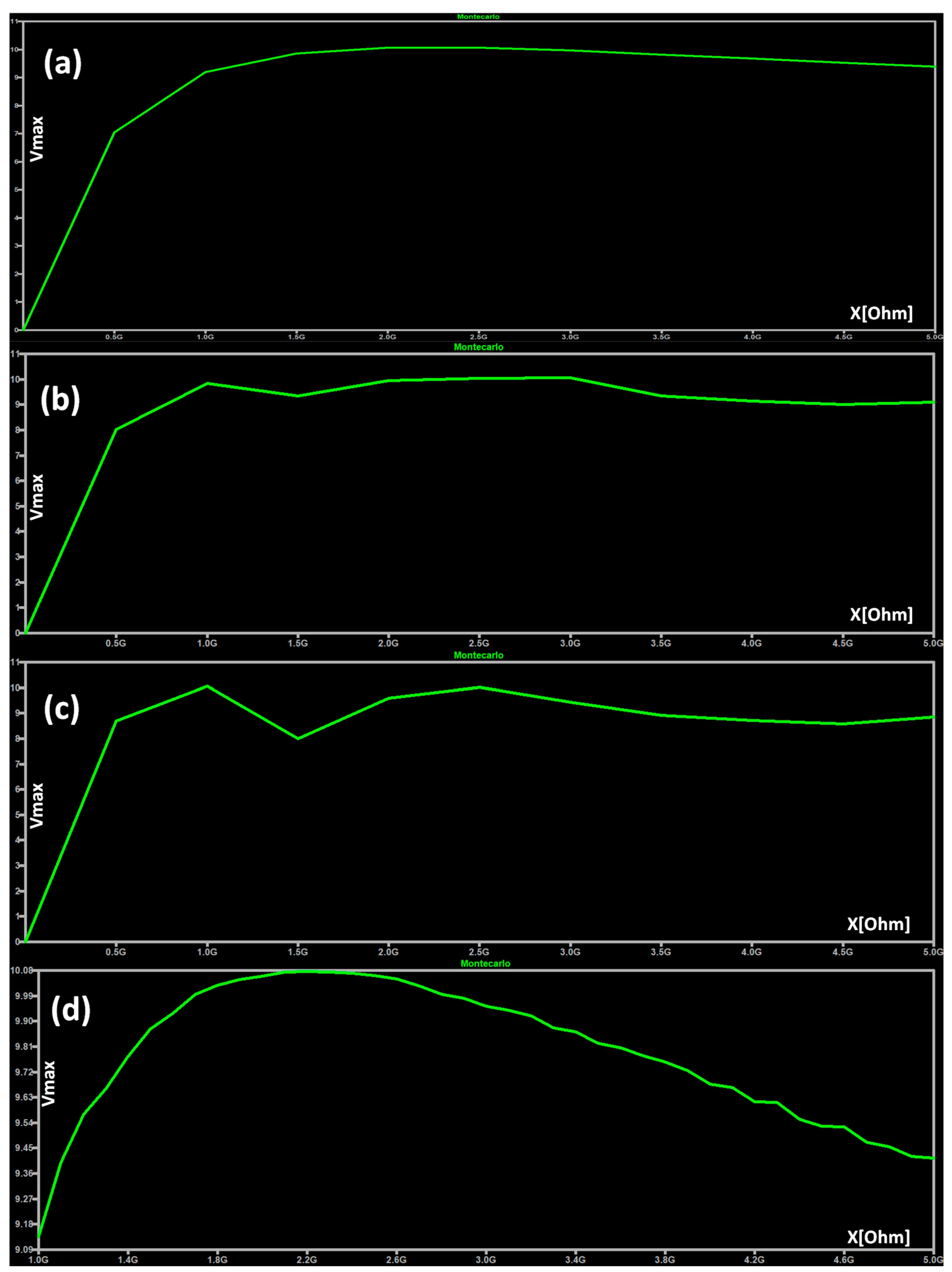
4.6.1. Circuit Stability: Monte Carlo Tolerance Analysis

In order to prove the high stability of the proposed circuit, a tolerance analysis is performed by means of the Monte Carlo approach. The LTSpice tool (version 24.1.0) [34] is appropriate to perform statistical tolerance analyses for complex circuits [60], as with the circuit in Figure 2. Specifically, the analysis is performed by changing the load at the output of the electrodes to estimate the circuit sensitivity/stability by observing the variation of the output voltage. In Figure 13 is illustrated the output voltage of the circuit in Figure 2 by executing the Monte Carlo parametric tolerance analysis by changing the load from 0.1 Ω to 5 GΩ and detecting the maximum output voltage peaks in the whole time domain interval. As observed in Figure 13, the lower loads are more susceptible to a flattening of the signal response. The response sensitivity is further analyzed by estimating and varying the tolerance parameter tol (tol = 0.015, tol = 0.5, tol = 1). The analysis is then focused on the lowest tolerance (the more stable condition) by increasing the steps of the parametric variation (Figure 14d) and estimating the statistical parameters of Table 9. The standard deviation (SD) is then compared in Table 10 to that of other studies concerning peak detection models; the smaller standard deviation of the proposed circuit model indicates that most of the data values are closer to the sample mean compared with other approaches characterized by data values that are more spread out (this indicates an easier reading of the peaks, even when using very low tolerances).

4.6.2. AI PCA

The Principal Component Analysis (PCA) is an exploratory analysis method providing a simplified interpretation of a multivariate dataset and used to decompose EEG signals. The goal is to apply this technique to RF and ANN models to find the directions of maximal variance (the principal components) projecting the input of different EEG signals into a space of a lower dimension while preserving maximum information. The use of interpolated electrodes could generate undesired ‘ghost’ signals [63] when the minimum eigenvalue λmin of the input data is smaller than a certain threshold, leading to matrix inversion failure. In Table 11 is the comparison between the minimum eigenvalue of the ANN and RF models and some reference eigenvalues found in the literature. The PCA is implemented by the ‘PCA Compute’ KNIME library.

5. Conclusions

The paper discusses an innovative AI-based DT model suitable as an alternative filtering approach to adjust possibly noisy EEG signals detected by electrodes. The proof of concept DT model is applied to prove the possibility of using AI for voltage signal trend correction when common white and Flicker noises alter the measured brain signal. The results highlight the possibility to attenuate the noise ripple behavior, thus mitigating the artifacts and cleaning the output voltage. The AI classification is adopted to facilitate the reading and to support results’ interpretation. Specifically, in order to demonstrate the functionality of the DT model, it is considered a specific EEG dataset characterized by alcoholic features. Furthermore, in order to reproduce real scenarios of EEG detection, the circuit model takes into account as the testing dataset real EEG signals by intentionally adding the noise effect. The RF algorithm is a good candidate to adjust the noisy voltage signal using the classification approach, and it is able to mitigate the accentuated ripple behavior. The proposed RF and ANN techniques have denoising performance similar to and slightly better than the traditional ones, such as bandpass filtering, FIR, and wavelet approaches. Specifically, the RF performance results prove that the RF could be a good alternative for the filtering process using a limited training dataset; RF exhibits a probabilistic error slightly lower than ANN, a slightly lower dispersion, and a better cleaning action. The presented EEG DT results could be further optimized by constructing a training dataset matching with more specific patient physiologic and clinical features. The followed approach could be adopted to construct other similar DT models processing generic biomedical signals and could be integrated with platforms detecting physiological signals using wearable devices.

Funding

This research received no external funding.

Data Availability Statement

Data are included in the paper.

Acknowledgments

The work has been developed within a framework of the Laboratory of the Dept. of Engineering of LUM University.

Conflicts of Interest

The authors declare no conflicts of interest.

Appendix A

The adopted KNIME workflow is illustrated in Figure A1. The workflow performs the RF and the ANN data processing, providing the classified EEG results as the predicted results. The main nodes are the following:
-
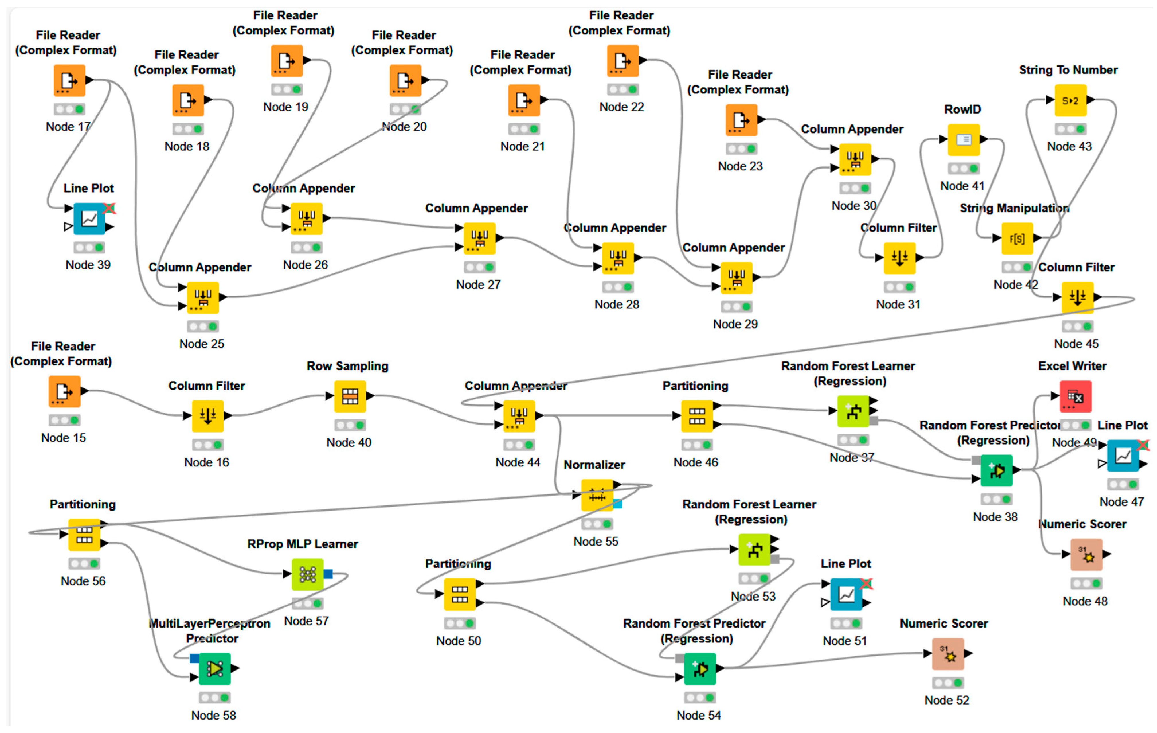
Input nodes importing the training dataset (seven tables) and the measured EEG signal (‘Excel Reader’);
-
Data pre-processing nodes: nodes merging tables (‘Column Appender’), nodes able to create the time variable (‘RowID’, ‘String Manipulation’, ‘String to Number’), nodes to clean unnecessary attributes (‘Column Filter’), node extracting a sample (a bunch of rows) from the input data to align the dataset dimensions of the testing dataset with the training dataset (‘Row Sampling’), and nodes splitting the dataset partition into training and testing AI nodes (‘Partitioning’);
-
AI training nodes (RF ‘Random Forest Learner’ and ANN ‘RProp MLP Learner’ nodes);
-
AI testing nodes (RF ‘Random Forest Predictor’ and ANN ‘Multilayer Perceptron Predictor’);
-
Error performance nodes (‘Numeric Score’);
-
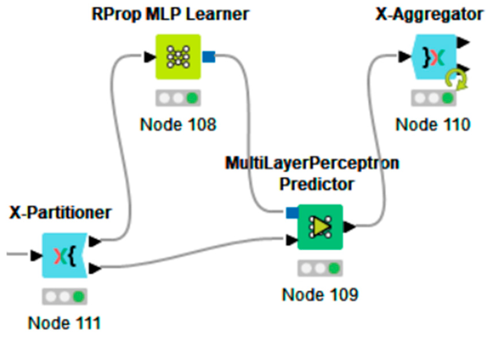
Cross-validation nodes (‘X-Partitioner’ and ‘X-Aggregator’ nodes of Figure A2);
-
Graphical dashboards’ nodes (‘Line Plot’).
In Figure A3 is illustrated an example of the tree model estimated during RF data processing performed by the workflow in Figure A1.
Figure A1. KNIME workflow used for RF and ANN EEG classification.
Electronics 14 01122 g0a1
Figure A2. Example of the KNIME nodes used for k-fold cross-validation (k = 10).
Electronics 14 01122 g0a2
Figure A3. Example of a tree model used for RF calculus.
Electronics 14 01122 g0a3
Figure A4 illustrates an example of the attenuation of EEG artifacts due to the movement of eyes using RF.
Figure A4. RF data processing: training without moving eyes and testing with eye movements. RF prediction attenuates the amplitudes due to eye movements according to the average EEG signal amplitude of the training dataset.
Electronics 14 01122 g0a4

References

  1. Gajare, M.; Shedge, D.K. CMOS Trans Conductance Based Instrumentation Amplifier for Various Biomedical Signal Analysis. Neuroquantology 2022, 11, 63–71. [Google Scholar] [CrossRef]
  2. Saptono, D.; Wahyudi, B.; Irawan, B. Design of EEG Signal Acquisition System Using Arduino MEGA1280 and EEGAnalyzer. MATEC Web Conf. 2016, 75, 04003. [Google Scholar] [CrossRef]
  3. Habibzadeh Tonekabony Shad, E.; Molinas, M.; Ytterdal, T. Impedance and Noise of Passive and Active Dry EEG Electrodes: A Review. IEEE Sens. J. 2020, 20, 14565–14577. [Google Scholar] [CrossRef]
  4. Benda, M.; Volosyak, I. Peak Detection with Online Electroencephalography (EEG) Artifact Removal for Brain–Computer Interface (BCI) Purposes. Brain Sci. 2019, 9, 347. [Google Scholar] [CrossRef] [PubMed]
  5. Lay-Ekuakille, A.; Griffo, G.; Massaro, A.; Spano, F.; Gigli, G. Experimental Characterization of an Implantable Neuro-Packaging for EEG Signal Recording and Measurement. Measurement 2016, 79, 321–330. [Google Scholar] [CrossRef]
  6. Alonso, E.; Giannetti, R.; Rodríguez-Morcillo, C.; Matanza, J.; Muñoz-Frías, J.D. A Novel Passive Method for the Assessment of Skin-Electrode Contact Impedance in Intraoperative Neurophysiological Monitoring Systems. Sci. Rep. 2020, 10, 2819. [Google Scholar] [CrossRef]
  7. Su, S.; Zhu, Z.; Wan, S.; Sheng, F.; Xiong, T.; Shen, S.; Hou, Y.; Liu, C.; Li, Y.; Sun, X.; et al. An ECG Signal Acquisition and Analysis System Based on Machine Learning with Model Fusion. Sensors 2023, 23, 7643. [Google Scholar] [CrossRef]
  8. Heikenfeld, J.; Jajack, A.; Rogers, J.; Gutruf, P.; Tian, L.; Pan, T.; Li, R.; Khine, M.; Kim, J.; Wang, J.; et al. Wearable Sensors: Modalities, Challenges, and Prospects. Lab Chip 2018, 18, 217–248. [Google Scholar] [CrossRef] [PubMed]
  9. Lay-Ekuakille, A.; Griffo, G.; Vergallo, P.; Massaro, A.; Spano, F.; Gigli, G. Implantable Neurorecording Sensing System: Wireless Transmission of Measurements. IEEE Sens. J. 2015, 15, 2603–2613. [Google Scholar] [CrossRef]
  10. Zhang, K.; Xu, G.; Du, C.; Wu, Y.; Zheng, X.; Zhang, S.; Han, C.; Liang, R.; Chen, R. Weak Feature Extraction and Strong Noise Suppression for SSVEP-EEG Based on Chaotic Detection Technology. IEEE Trans. Neural Syst. Rehabil. Eng. 2021, 29, 862–871. [Google Scholar] [CrossRef]
  11. Eltrass, A.S.; Ghanem, N.H. A New Automated Multi-Stage System of Non-Local Means and Multi-Kernel Adaptive Filtering Techniques for EEG Noise and Artifacts Suppression. J. Neural Eng. 2021, 18, 036023. [Google Scholar] [CrossRef]
  12. Kaur, C.; Bisht, A.; Singh, P.; Joshi, G. EEG Signal Denoising Using Hybrid Approach of Variational Mode Decomposition and Wavelets for Depression. Biomed. Signal Process. Control 2021, 65, 102337. [Google Scholar] [CrossRef]
  13. Jindal, K.; Upadhyay, R.; Singh, H.S. Application of Hybrid GLCT-PICA de-Noising Method in Automated EEG Artifact Removal. Biomed. Signal Process. Control 2020, 60, 101977. [Google Scholar] [CrossRef]
  14. Porr, B.; Daryanavard, S.; Bohollo, L.M.; Cowan, H.; Dahiya, R. Real-Time Noise Cancellation with Deep Learning. PLoS ONE 2022, 17, e0277974. [Google Scholar] [CrossRef] [PubMed]
  15. Amer, N.S.; Belhaouari, S.B. Exploring New Horizons in Neuroscience Disease Detection through Innovative Visual Signal Analysis. Sci. Rep. 2024, 14, 4217. [Google Scholar] [CrossRef]
  16. Lv, Z.; Qiao, L.; Lv, H. Cognitive Computing for Brain–Computer Interface-Based Computational Social Digital Twins Systems. IEEE Trans. Comput. Soc. Syst. 2022, 9, 1635–1643. [Google Scholar] [CrossRef]
  17. Takahashi, Y.; Idei, H.; Komatsu, M.; Tani, J.; Tomita, H.; Yamashita, Y. Digital Twin Brain Simulator: Harnessing Primate ECoG Data for Real-Time Consciousness Monitoring and Virtual Intervention. bioRxiv 2024. [Google Scholar] [CrossRef]
  18. Falkowski, P.; Osiak, T.; Wilk, J.; Prokopiuk, N.; Leczkowski, B.; Pilat, Z.; Rzymkowski, C. Study on the Applicability of Digital Twins for Home Remote Motor Rehabilitation. Sensors 2023, 23, 911. [Google Scholar] [CrossRef]
  19. Nishida, S.; Nakamura, M.; Ikeda, A.; Shibasaki, H. Signal Separation of Background EEG and Spike by Using Morphological Filter. Med. Eng. Phys. 1999, 21, 601–608. [Google Scholar] [CrossRef]
  20. Pyrzowski, J.; Siemiński, M.; Sarnowska, A.; Jedrzejczak, J.; Nyka, W.M. Interval Analysis of Interictal EEG: Pathology of the Alpha Rhythm in Focal Epilepsy. Sci. Rep. 2015, 5, 16230. [Google Scholar] [CrossRef]
  21. Ruiz de Miras, J.; Derchi, C.-C.; Atzori, T.; Mazza, A.; Arcuri, P.; Salvatore, A.; Navarro, J.; Saibene, F.L.; Meloni, M.; Comanducci, A. Spatio-Temporal Fractal Dimension Analysis from Resting State EEG Signals in Parkinson’s Disease. Entropy 2023, 25, 1017. [Google Scholar] [CrossRef] [PubMed]
  22. Olejarczyk, E.; Sobieszek, A.; Assenza, G. Automatic Detection of the EEG Spike–Wave Patterns in Epilepsy: Evaluation of the Effects of Transcranial Current Stimulation Therapy. Int. J. Mol. Sci. 2024, 25, 9122. [Google Scholar] [CrossRef] [PubMed]
  23. Gemein, L.A.W.; Schirrmeister, R.T.; Chrabąszcz, P.; Wilson, D.; Boedecker, J.; Schulze-Bonhage, A.; Hutter, F.; Ball, T. Machine-Learning-Based Diagnostics of EEG Pathology. Neuroimage 2020, 220, 117021. [Google Scholar] [CrossRef]
  24. Houssein, E.H.; Hammad, A.; Ali, A.A. Human Emotion Recognition from EEG-Based Brain–Computer Interface Using Machine Learning: A Comprehensive Review. Neural Comput. Appl. 2022, 34, 12527–12557. [Google Scholar] [CrossRef]
  25. Attar, E.T. Review of Electroencephalography Signals Approaches for Mental Stress Assessment. Neurosciences 2022, 27, 209–215. [Google Scholar] [CrossRef]
  26. Shen, M.; Wen, P.; Song, B.; Li, Y. Detection of Alcoholic EEG Signals Based on Whole Brain Connectivity and Convolution Neural Networks. Biomed. Signal Process. Control 2023, 79, 104242. [Google Scholar] [CrossRef]
  27. Neeraj; Singhal, V.; Mathew, J.; Behera, R.K. Detection of Alcoholism Using EEG Signals and a CNN-LSTM-ATTN Network. Comput. Biol. Med. 2021, 138, 104940. [Google Scholar] [CrossRef]
  28. Agarwal, S.; Zubair, M. Classification of Alcoholic and Non-Alcoholic EEG Signals Based on Sliding-SSA and Independent Component Analysis. IEEE Sens. J. 2021, 21, 26198–26206. [Google Scholar] [CrossRef]
  29. Baijal, S.; Singh, S.; Rani, A.; Agarwal, S. Performance Evaluation of S-Golay and MA Filter on the Basis of White and Flicker Noise. In Advances in Intelligent Systems and Computing; Springer International Publishing: Cham, Switzerland, 2016; pp. 245–255. [Google Scholar]
  30. Massaro, A. Artificial Intelligence Signal Control in Electronic Optocoupler Circuits Addressed on Industry 5.0 Digital Twin. Electronics 2024, 13, 4543. [Google Scholar] [CrossRef]
  31. Chi, Y.M.; Jung, T.-P.; Cauwenberghs, G. Dry-Contact and Noncontact Biopotential Electrodes: Methodological Review. IEEE Rev. Biomed. Eng. 2010, 3, 106–119. [Google Scholar] [CrossRef]
  32. Huigen, E.; Peper, A.; Grimbergen, I.C.A.; Samenvatting. Noise in Biopotential Recording Using Surface Electrodes; Technical Report; University of Amsterdam: Amsterdam, The Netherlands, 2000. [Google Scholar]
  33. Voss, R.F.; Clarke, J. Flicker (1f) Noise: Equilibrium Temperature and Resistance Fluctuations. Phys. Rev. 1976, 13, 556–573. [Google Scholar] [CrossRef]
  34. LTspice. Available online: https://www.analog.com/en/resources/design-tools-and-calculators/ltspice-simulator.html (accessed on 17 December 2024).
  35. LTspiceNoiseSources. Available online: https://github.com/yildi1337/LTspiceNoiseSources (accessed on 17 December 2024).
  36. EEG-Alcohol. Available online: https://www.kaggle.com/datasets/nnair25/Alcoholics (accessed on 17 December 2024).
  37. KNIME. Available online: https://www.knime.com/ (accessed on 17 December 2024).
  38. Massaro, A. Electronics in Advanced Research Industries: Industry 4.0 to Industry 5.0 Advances; Wiley: Hoboken, NJ, USA, 2021. [Google Scholar] [CrossRef]
  39. Sabio, J.; Williams, N.S.; McArthur, G.M.; Badcock, N.A. A Scoping Review on the Use of Consumer-Grade EEG Devices for Research. PLoS ONE 2024, 19, e0291186. [Google Scholar] [CrossRef] [PubMed]
  40. LaRocco, J.; Le, M.D.; Paeng, D.-G. A Systemic Review of Available Low-Cost EEG Headsets Used for Drowsiness Detection. Front. Neuroinform. 2020, 14, 553352. [Google Scholar] [CrossRef]
  41. Jaros, R.; Barnova, K.; Vilimkova Kahankova, R.; Pelisek, J.; Litschmannova, M.; Martinek, R. Independent Component Analysis Algorithms for Non-Invasive Fetal Electrocardiography. PLoS ONE 2023, 18, e0286858. [Google Scholar] [CrossRef] [PubMed]
  42. Safieddine, D.; Kachenoura, A.; Albera, L.; Birot, G.; Karfoul, A.; Pasnicu, A.; Biraben, A.; Wendling, F.; Senhadji, L.; Merlet, I. Removal of Muscle Artifact from EEG Data: Comparison between Stochastic (ICA and CCA) and Deterministic (EMD and Wavelet-Based) Approaches. EURASIP J. Adv. Signal Process. 2012, 2012, 127. [Google Scholar] [CrossRef]
  43. Cataldo, A.; Criscuolo, S.; De Benedetto, E.; Masciullo, A.; Pesola, M.; Schiavoni, R.; Invitto, S. A Method for Optimizing the Artifact Subspace Reconstruction Performance in Low-Density EEG. IEEE Sens. J. 2022, 22, 21257–21265. [Google Scholar] [CrossRef]
  44. Alyasseri, Z.A.A.; Khader, A.T.; Al-Betar, M.A.; Abasi, A.K.; Makhadmeh, S.N. EEG Signals Denoising Using Optimal Wavelet Transform Hybridized with Efficient Metaheuristic Methods. IEEE Access 2020, 8, 10584–10605. [Google Scholar] [CrossRef]
  45. Bajpai, B.K.; Zakelis, R.; Deimantavicius, M.; Imbrasiene, D. Comparative Study of Novel Noninvasive Cerebral Autoregulation Volumetric Reactivity Indices Reflected by Ultrasonic Speed and Attenuation as Dynamic Measurements in the Human Brain. Brain Sci. 2020, 10, 205. [Google Scholar] [CrossRef]
  46. Bastianini, S.; Alvente, S.; Berteotti, C.; Lo Martire, V.; Silvani, A.; Swoap, S.J.; Valli, A.; Zoccoli, G.; Cohen, G. Accurate Discrimination of the Wake-Sleep States of Mice Using Non-Invasive Whole-Body Plethysmography. Sci. Rep. 2017, 7, 41698. [Google Scholar] [CrossRef]
  47. Mariani, S.; Tarokh, L.; Djonlagic, I.; Cade, B.E.; Morrical, M.G.; Yaffe, K.; Stone, K.L.; Loparo, K.A.; Purcell, S.M.; Redline, S.; et al. Evaluation of an Automated Pipeline for Large-Scale EEG Spectral Analysis: The National Sleep Research Resource. Sleep Med. 2018, 47, 126–136. [Google Scholar] [CrossRef]
  48. Levendowski, D.J.; Popovic, D.; Berka, C.; Westbrook, P.R. Retrospective Cross-Validation of Automated Sleep Staging Using Electroocular Recording in Patients with and without Sleep Disordered Breathing. Int. Arch. Med. 2012, 5, 21. [Google Scholar] [CrossRef] [PubMed]
  49. Apicella, A.; Arpaia, P.; Mastrati, G.; Moccaldi, N. EEG-Based Detection of Emotional Valence towards a Reproducible Measurement of Emotions. Sci. Rep. 2021, 11, 21615. [Google Scholar] [CrossRef]
  50. Alyasseri, Z.A.A.; Khader, A.T.; Al-Betar, M.A. Electroencephalogram Signals Denoising Using Various Mother Wavelet Functions: A Comparative Analysis. In Proceedings of the International Conference on Imaging, Signal Processing and Communication, Penang, Malaysia, 26–28 July 2017; ACM: New York, NY, USA, 2017; pp. 100–105. [Google Scholar]
  51. St. Louis, E.K.; Frey, L.C.; Britton, J.W.; Hopp, J.L.; Korb, P.; Koubeissi, M.Z.; Lievens, W.E.; Pestana-Knight, E.M. EEG in the Epilepsies; American Epilepsy Society: Chicago, IL, USA, 2016. [Google Scholar]
  52. Gimenez-Aparisi, G.; Guijarro-Estelles, E.; Chornet-Lurbe, A.; Ballesta-Martinez, S.; Pardo-Hernandez, M.; Ye-Lin, Y. Early Detection of Parkinson’s Disease: Systematic Analysis of the Influence of the Eyes on Quantitative Biomarkers in Resting State Electroencephalography. Heliyon 2023, 9, e20625. [Google Scholar] [CrossRef]
  53. Hallett, M.; DelRosso, L.M.; Elble, R.; Ferri, R.; Horak, F.B.; Lehericy, S.; Mancini, M.; Matsuhashi, M.; Matsumoto, R.; Muthuraman, M.; et al. Evaluation of Movement and Brain Activity. Clin. Neurophysiol. 2021, 132, 2608–2638. [Google Scholar] [CrossRef] [PubMed]
  54. McDonald, C.; El Yaakoubi, N.A.; Lennon, O. Brain (EEG) and Muscle (EMG) Activity Related to 3D Sit-to-Stand Kinematics in Healthy Adults and in Central Neurological Pathology—A Systematic Review. Gait Posture 2024, 113, 374–397. [Google Scholar] [CrossRef] [PubMed]
  55. Gordleeva, S.Y.; Lobov, S.A.; Grigorev, N.A.; Savosenkov, A.O.; Shamshin, M.O.; Lukoyanov, M.V.; Khoruzhko, M.A.; Kazantsev, V.B. Real-Time EEG–EMG Human–Machine Interface-Based Control System for a Lower-Limb Exoskeleton. IEEE Access 2020, 8, 84070–84081. [Google Scholar] [CrossRef]
  56. Wang, Y.; Gotman, J. The Influence of Electrode Location Errors on EEG Dipole Source Localization with a Realistic Head Model. Clin. Neurophysiol. 2001, 112, 1777–1780. [Google Scholar] [CrossRef]
  57. Eye State Classification EEG Dataset. Available online: https://www.kaggle.com/datasets/robikscube/eye-state-classification-eeg-dataset/data (accessed on 26 February 2025).
  58. Massaro, A.; Lay-Ekuakille, A. Analysis of Magnetic Field Impact on Nanoparticles Used in Nanomedicine and a Measurement Approach. Measurement 2024, 226, 114167. [Google Scholar] [CrossRef]
  59. Massaro, A.; Cazzato, G.; Ingravallo, G.; Casatta, N.; Lupo, C.; Vacca, A.; Iannone, F.; Girolamo, F. Pre-Screening of Endomysial Microvessel Density by Fast Random Forest Image Processing Machine Learning Algorithm Accelerates Recognition of a Modified Vascular Network in Idiopathic Inflammatory Myopathies. Diagn. Pathol. 2025, 20, 13. [Google Scholar] [CrossRef]
  60. Knudtsen, S. How to Model Statistical Tolerance Analysis for Complex Circuits Using LTspice. Available online: https://www.analog.com/en/resources/technical-articles/how-to-model-statistical-tolerance-analysis.html (accessed on 4 March 2025).
  61. Adam, A.; Ibrahim, Z.; Mokhtar, N.; Shapiai, M.I.; Cumming, P.; Mubin, M. Evaluation of Different Time Domain Peak Models Using Extreme Learning Machine-Based Peak Detection for EEG Signal. Springerplus 2016, 5, 1036. [Google Scholar] [CrossRef]
  62. Krzysztof, P.; Kolodiy, Z.; Yatsyshyn, S.; Majewski, J.; Khoma, Y.; Petrovska, I.; Lasarenko, S.; Hut, T. Standard deviation in the simulation of statistical measurements. Metrol. Meas. Syst. 2023, 30, 17–30. [Google Scholar] [CrossRef]
  63. Kim, H.; Luo, J.; Chu, S.; Cannard, C.; Hoffmann, S.; Miyakoshi, M. ICA’s Bug: How Ghost ICs Emerge from Effective Rank Deficiency Caused by EEG Electrode Interpolation and Incorrect Re-Referencing. Front. Signal Process. 2023, 3, 1064138. [Google Scholar] [CrossRef]
Figure 1. EEG DT model based on AI EEG signal classification cleaning the noisy brain signal. Vn indicates the Flicker noise and the white noise generator sources coupled at the input of the amplification system. The scheme is representative of a bipolar configuration using a ground link as the electrical reference.
Electronics 14 01122 g001
Figure 2. LTSpice circuit modeling a couple of EEG electrodes influenced simultaneously by Flicker and white noises. The brain voltage signals (brain voltage 1 and brain voltage 2) use a ground link as the electrical reference.
Electronics 14 01122 g002
Figure 3. LTSpice simulation of the Flicker noise effect for the frequency band (effect of the generators Vn of U1 and U4 of Figure 2).
Electronics 14 01122 g003
Figure 4. LTSpice results of the circuit model of Figure 2: (a) single alcoholic EEG trend (brain blue signal V(n006)) coupled at the input of the electrode and the simulated noisy signal at the output of the whole circuit (green voltage output plot V(out) reproducing the noisy detection); (b) frequency responses of the input signal (blue plot) and of the whole circuit output (green plot).
Electronics 14 01122 g004
Figure 5. LTSpice results of the circuit model of Figure 2: alcoholic EEG signals (brain voltage 1 coupled with electrode 1 and brain voltage 2 coupled with the electrode 2) and the output voltage (Vout) without noises (a) and with noises (b). The EEG measurements refer to the Fp configuration.
Electronics 14 01122 g005
Figure 6. KNIME results: comparison between (a) the noisy brain signal V(out) and the original EEG one; (b) the RF-predicted signal (Predicted(Vout)) and the EEG one; (c) the noisy brain signal V(out) and the RF-predicted signal (Predicted(Vout)); (d) the noisy brain signal V(out) of the original EEG and the RF-predicted one (Predicted(Vout)).
Electronics 14 01122 g006
Figure 7. KNIME-normalized results: comparison between normalized RF-predicted, ANN-predicted, and EEG alcoholic normalized signals.
Electronics 14 01122 g007
Figure 8. KNIME-normalized results: comparison between (a) the noisy brain signal V(out) and the original EEG one; (b) the RF-predicted signal (Predicted(Vout)) and the EEG one; (c) the noisy brain signal V(out) and the RF-predicted signal (Predicted(Vout)); (d) the noisy brain signal V(out) of the original EEG and the RF-predicted one (Predicted(Vout)).
Electronics 14 01122 g008
Figure 9. KNIME-normalized results performed for a double input brain signal (Fp configuration): comparison between EEG input clean signal with ANN- and RF-predicted output voltages estimated for a noisy condition.
Electronics 14 01122 g009
Figure 10. KNIME-normalized results performed for a double input brain signal (Fp configuration): comparison between an EEG clean input signal with an EEG noisy one and RF output voltage prediction estimated for a noisy condition.
Electronics 14 01122 g010
Figure 11. (ac) Bland–Altman plots comparing EEG measurements with RF-predicted results. (df) Bland–Altman plots comparing EEG measurements with ANN-predicted results. The blue line indicates the bias, and the red line indicates the upper and the lower limits of agreement. A are the values of the x-axis of Equation (3). B are the values of the y-axis of Equation (4).
Electronics 14 01122 g011
Figure 12. Roadmap of the clinical protocol for implementing the proposed DT-AI EEG.
Electronics 14 01122 g012
Figure 13. Monte Carlo parametric simulation varying the output load R9 (R9 ranging from 0.1 Ω to 5 GΩ) of the electronic system of Figure 2. Inset: output of the LTSpice circuit implementing the Monte Carlo function.
Electronics 14 01122 g013
Figure 14. Monte Carlo parametric tolerance analysis performed for tolerance parameter (a) tol = 0.015, (b) tol = 0.5, (c) tol = 1, and (d) fitting the R9 parameter, ranging from 1 GΩ to 5 GΩ, for tol = 0.015 (resistance steps of 0.1 GΩ).
Electronics 14 01122 g014
Table 1. Electrical parameters [3,5] of the DT circuit model of Figure 2.
StageValue
SkinR1 = 1 MΩ; RS = 1 MΩ; CS = 10 nF
Skin/electrodeRSe = 1 kΩ; CSe = 10 nF
ElectrodeRe = 35 kΩ; CSe = 10 nF
AmplificationIdeal operational amplifier
Table 2. Statistical performances of the RF and ANN algorithms.
ParameterRFANN
R2 (coefficient of determination)0.3780.344
Mean Absolute Error (MAE)0.080.134
Mean Squared Error (MSE)0.010.028
Root Mean Squared Error (RMSE)0.01230.166
Mean Signed Difference (MSD)−0.0050.037
Table 3. K-fold cross-validation test of the RF and ANN algorithms (MSE values for k = 10 folds).
FoldRFANN
10.020.027
20.0180.028
30.010.03
40.0160.026
50.0240.031
60.0170.022
70.0130.021
80.0180.021
90.0190.02
100.0150.028
Table 4. Advantages and disadvantages of the tools and methodologies proposed in the EEG DT.
Proposed MethodologyAdvantagesDisadvantages
Circuit simulationThe circuit simulation provides the testing dataset to use for the classification process of the AI-supervised algorithm. The possibility to replicate real noise conditions allows the prediction of possible uncontrollable signal trend behaviors.The circuital electrical and electronic parameters (resistances and capacitance of Table 1) could vary, consecutively changing the simulation output. In order to mitigate this effect, it is possible to perform a parametric simulation by studying the electrical parameters’ sensitivity versus the noisy trend of the voltage output.
Dataset samplingPossibility to classify the sampled brain signal based on the region where the electrode is applied (F, Fp, T, C, P, O, A). The data sampling is a characteristic of the adopted technology.The sampling of the circuit DT simulator should be aligned with the sampling of the adopted electrode technology to avoid losing significant data (important peak positions or significant trends).
Training dataset of the supervised AI algorithmThe preliminary selection of a dataset of a specific pathology or known EEG signal trends (as in the case of the paper related to EEG alcoholic signals) will optimize the training model to recognize the class of a specific EEG morphology.The AI-supervised algorithms require a significant selection of training EEG datasets, including information regarding electrode application with reference to brain regions.
Quasi real-time EEG detectionThe application of the DT model could correct in real time the EEG signal due to a wrong measurement affected by Flicker and white noises.The model does not provide information about the origin of the noises to understand if the EEG technology is still suitable for measurements.
DT dashboards and performance indicatorsThe dashboards of Figure 3, Figure 4, Figure 5, Figure 6 and Figure 7 and the error indicators of Table 2 (MAE, MSE, MSD, RMSE) are fundamental to checking the DT’s behavior and its performance during parameter setting.The dashboards and the indicators refer to a specific supervised algorithm. It is not possible to decide a priori the best algorithm to apply, and this entails the need to compare different DT models (see Figure 6).
Table 5. Limitations and perspectives of important properties of the EEG DT model.
DT PropertyLimitsPerspectives
Tools’ integrationA stable DT requires a fully integrated DT platform composed by the technology, the circuit simulator, and the AI engine. A limit of a non-integrated platform is the need to manipulate the dataset to align and balance the dataset homogeneously (for example, by fixing the number of records). This aspect could lead to the deletion of some records and, therefore, a lack of information to process (possible missed peaks or unseen trends).A fully integrated DT platform, including hardware (electrode systems) and software (circuit simulator), allows for fixing the EEG sampling rate, thus facilitating the construction of a homogeneous dataset.
Application of the DT model to new measurementsThe EEG model is applied in the proposed paper to an open dataset [35] to prove the DT ‘proof of concept’. The EEG DT should be set for a specific electrode technology which could lead to a significant change of the circuital parameters and of hyper-parameters according with new measurements. The EEG DT could be applied to specific electrodes to customize the settings of the DT model.
Checks of EEG trend variationsThe proposed DT model does not provide an automatic check of the comparison of the predicted results with the EEG input ones (the presence or absence of peaks, matching or mismatching of the voltage morphology).An automatic check system could facilitate data interpretation and, in general, the reading of the output signal, thus accelerating EEG diagnosis.
Comparison between circuit simulation results and real measurementsThe EEG DT model is applied to replicate and simulate a noisy signal. The simulation should be compared with the real noisy signal before to apply the ‘cleaning’ process by the AI-supervised algorithms.Future work will address the definition of a procedure to compare the simulated EEG results with the detected EEG measurements.
Table 6. Bland–Altman statistical parameters.
MeasurementANNRF
1Bias = −0.012
SD = 0.203
Bias = −0.017
SD = 0.165
2Bias = 0.005
SD = 0.051
Bias = −0.001
SD = 0.0545
3Bias = −0.004
SD = 0.063
Bias = −0.001
SD = 0.074
4Bias = 0.004
SD = 0.0305
Bias = −0.006
SD = 0.036
5Bias = 0.004
SD = 0.177
Bias = 0.01
SD = 0.1385
6Bias = 0.02
SD = 0.144
Bias = 0.012
SD = 0.137
7Bias = 0.016
SD = 0.0685
Bias = 0.008
SD = 0.1005
8Bias = −0.012
SD = 0.054
Bias = −0.009
SD = 0.0525
Table 7. Comparison between average SD of ANN and RF and SD using filtering approaches.
Average SD (ANN)Average SD
(RF)
SD
Bandpass Filtering [45]
SD
FIR Filtering [45]
0.09880.09470.16470.1382
Table 8. Comparison between the MSE estimated in this work (ANN and RF) and the MSE related to the denoising process using wavelet functions.
ANN (This Work)RF (This Work)Wavelet Functions Denoising PLN [50]Wavelet Functions
Denoising EMG [50]
Wavelet Functions
Denoising 15 dB WGN [50]
0.0200.010≅0.02≅0.012≅26.72
Table 9. Statistical parameters of the performed Monte Carlo tolerance analysis of Figure 14d.
MinMaxMeanSt. Deviation (SD)VarianceSkewnessKurtosis
9.13710.0759.7870.2430.059−0.611−0.432
Table 10. Standard deviation (SD) comparison.
SD
Monte Carlo
(This Work)
SD Dumpala Peak Model [61]SD Acir Peak Model [61]SD Liu Peak Model [61]SD Dongle Peak Model [61]SD [62] *
(∆t = 1 s)
0.2431.41.42.60.90.803
* Includes the Flicker and the white noise analysis.
Table 11. Comparison of minimum eigenvalues λmin.
ANN *
(This Work)
RF *
(This Work)
Threshold [63]Normal
Decomposition
Obtained [63]
7.82 × 10−47.9 × 10−610−7100
* Eigenvalues estimated in the case of the best hyper-parameters.
Disclaimer/Publisher’s Note: The statements, opinions and data contained in all publications are solely those of the individual author(s) and contributor(s) and not of MDPI and/or the editor(s). MDPI and/or the editor(s) disclaim responsibility for any injury to people or property resulting from any ideas, methods, instructions or products referred to in the content.

