HRRnet: A Parameter Estimation Method for Linear Frequency Modulation Signals Based on High-Resolution Spectral Line Representation

Abstract

Under the condition of low SNR, enhancing the precision of parameter estimation for linear frequency modulation (LFM) signals and diminishing the complexity of the relevant methods represent crucial challenges that are presently being confronted. To address this problem, a parameter estimation method for LFM signals based on the High-Resolution Representation network (HRRnet) is proposed. The fundamental concept underlying this method lies in the employment of a strategy that combines the expansion of the receptive field with the fusion of multi-scale features. This enables the efficient extraction of both global and local information, which in turn augments the expressive power of the inherent signal characteristics and consequently mitigates the impact of noise interference. Based on this strategy, a high-resolution representation of the time–frequency spectrum of the signals is performed to improve the distinguishability of the time–frequency spectrum, and it further improve the accuracy of parameter estimation for LFM signals. In addition, the network utilizes dilated convolution to expand the receptive field while reducing the dependence on network depth, so as to control the network complexity and further optimize the computational efficiency. Experimental results show that when the SNR is greater than −12 dB and the tolerable error is equal to 0.1, the average accuracy of the HRRnet method for estimating the initial frequency and frequency modulation coefficient of LFM signals can reach above 95.53% and 91.19%, respectively, and its number of parameters and computational complexity are reduced to more than 20.47% and 20.37% of those of the existing methods.

1. Introduction

As a highly significant detection means in modern technology, radar [1,2] is widely applied in both military and civilian fields. In the military realm, radar serves as a crucial tool for strategic defense, battlefield awareness, and weapon guidance, being of vital importance to national security and combat effectiveness. In civilian applications, it is an essential support for air traffic control, navigation safety at sea, meteorological monitoring and forecasting, and resource and environmental monitoring, ensuring smooth transportation, safe living, and effective resource management.

The LFM signal is a time-varying non-stationary broadband signal, characterized by strong anti-jamming capabilities and high range resolution. It finds extensive applications in multiple fields such as acoustics, radar, and electronic information countermeasures. Particularly in the radar field, the LFM signal plays a key role in target detection, imaging, etc., by virtue of its unique advantages. For instance, in synthetic aperture radar (SAR) [3], the LFM signal enables high-resolution imaging, clearly revealing target details. The LFM signal can meet various functional requirements by adjusting the initial frequency and frequency modulation coefficient according to different application scenarios. Therefore, the estimation of LFM signal parameters is of great significance for the precise analysis and effective processing of the signal [4].

Currently, the traditional parameter estimation methods for LFM signals mainly include the time–frequency (TF) [5,6] analysis method and the Fractional Fourier Transform (FrFT) analysis method [7,8,9]. The TF analysis method uses the Short-Time Fourier Transform (STFT) [10,11] or the Wigner–Ville Distribution (WVD) [12,13] to convert the signal from the one-dimensional time domain to the two-dimensional time–frequency domain, and further employs linear detection methods such as the Radon [14] or Hough [15] transform to estimate the initial frequency and frequency-modulation factor of the frequency-modulated signal. The FrFT analysis method selects an appropriate transformation order to make the energy of a specific signal highly concentrated on the basis vectors in the fractional domain. The energy distribution after transformation can exhibit obvious pulse characteristics, and then the signal parameters are estimated by searching for the positions of the energy pulses.

Typically, both the TF analysis method and the FrFT analysis method are capable of effectively estimating the initial frequency and frequency modulation coefficient of LFM signals. However, in situations where there is a low SNR and a limited number of sampling points, the TF analysis method experiences a deterioration in the quality of the time–frequency diagram as a result of noise interference. This deterioration is manifested as energy dispersion and blurring, which renders it challenging to extract the inherent information of LFM signals and consequently impacts the accuracy of parameter estimation. By contrast, the FrFT analysis method has the ability to boost the signal energy at specific locations within the fractional domain and mitigate the noise, thereby possessing relatively robust anti-noise capabilities. Nonetheless, its performance remains constrained by factors like the length of the signal and the quantity of sampling points, which will inevitably impose certain limitations on its application within practical scenarios.

Neural networks are capable of capturing signal features at different scales. When dealing with linear frequency-modulated signals, they can not only capture subtle local frequency changes but also grasp the overall frequency evolution trend. The multi-scale features complement each other, enabling a more comprehensive description of the signals. Compared with the single-scale feature extraction of traditional methods, the multi-scale features extracted by neural networks can improve the accuracy of signal parameter estimation. Even in complex environments, neural networks can analyze signals more effectively, providing more reliable support for fields such as radar and communication that rely on signal processing. This is conducive to achieving more accurate signal analysis and processing.

In recent years, the data-driven neural network technology [16] has been booming in the field of signal processing. With its powerful feature extraction ability and excellent nonlinear expressiveness, it has shown remarkable effects, providing new research ideas and technical approaches for the estimation of LFM signal parameters. Chen et al. [17] used deep neural network technology to replace the traditional TF transform method and the FrFT method to achieve the estimation of frequency modulation signal parameters, greatly improving the accuracy of parameter estimation under the same conditions. Ben, G. et al. [18] proposed a frequency modulation signal parameter estimation method based on neural network noise reduction. This method uses a multi-layer convolutional neural network to reduce the noise of the LFM signal and combines the TF analysis method and the FrFT analysis method to estimate the initial frequency and frequency modulation coefficient, proving that the multi-layer neural network has good noise reduction ability. Su, H. et al. [19] used the WVD method to map the time-domain signal to the time–frequency domain, constructed a multi-layer complex convolution (Complex Value Convolutional, CVC) to extract the time–frequency domain features of the signal, achieved the estimation of signal parameters, and demonstrated the effectiveness of the complex convolutional neural network for feature extraction.

It is noteworthy that existing methods generally expand the receptive field of features and enhance the multi-scale characteristics by increasing the network depth and the number of channels to improve the network’s ability to extract signal features. However, such a strategy will significantly increase the complexity of the network, thus reducing the efficiency of parameter estimation. In addition, due to the influence of noise interference and the limitation of the number of sampling points, the resolution in the time–frequency domain will decrease, further reducing the accuracy of the method for parameter estimation. To address the above problems, this paper proposes the High-Resolution Representation network (HRRnet) for estimating the parameters of LFM signals. With enhanced feature extraction ability and reduced network complexity as the core starting points, this network relies on the effective extraction of the inherent characteristics of the signal to achieve the purposes of signal denoising and high-resolution spectral line representation, thus realizing the accurate estimation of the parameters of LFM signals under a low SNR.

The structure of the remaining part of this paper is as follows. Firstly, Section 1 presents the related work on using neural networks for noise reduction and high-resolution signal representation in low-SNR scenarios. Subsequently, Section 2 elaborates on the design and parameter optimization of HRRnet. The simulation experiments and result analysis are conducted in Section 3. Finally, the conclusions are drawn in Section 4.

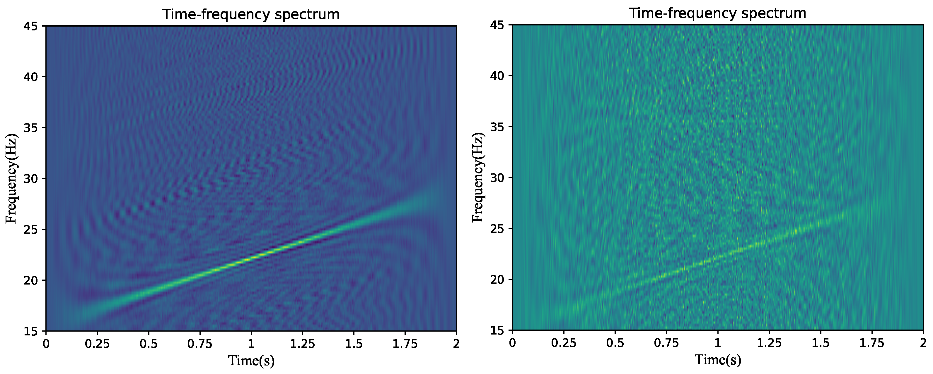
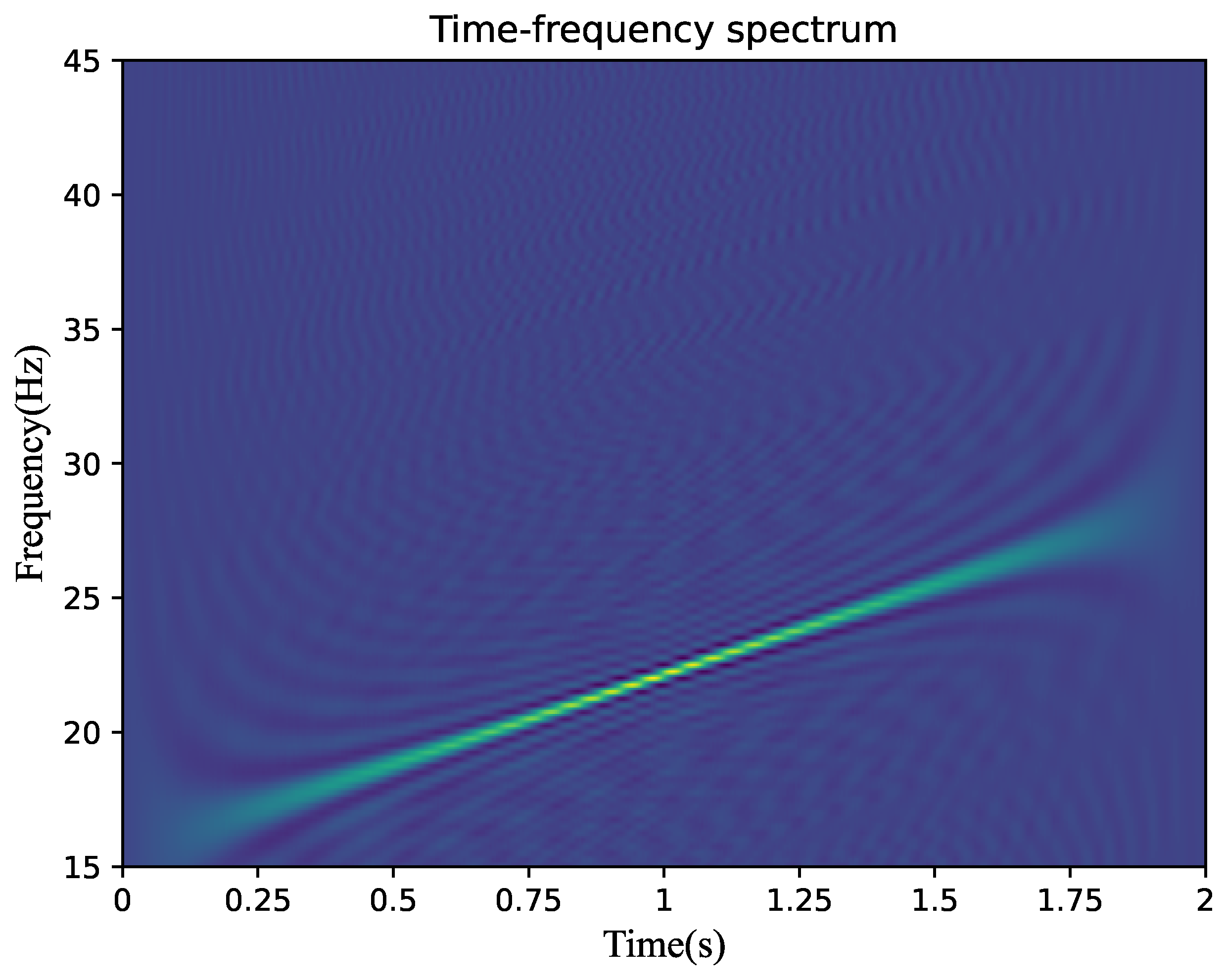
2. Signal Denoising and High-Resolution Representation of the Time–Frequency Spectrum

In the context of a low SNR, the substantial noise interference tends to obscure the intrinsic characteristics of the signal, making it difficult to directly estimate the parameters of the signal [20]. Drawing inspiration from the neural network-based image denoising methodologies [21,22], the employment of neural networks for signal denoising exhibits a high degree of feasibility.

Figure 1 presents the time–frequency analysis diagrams of the LFM signal when the SNRs are 0 dB and −10 dB. From a global perspective: There is a linear relationship between time and frequency. Meanwhile, as the noise energy increases, the signal characteristics become increasingly blurred. By expanding the receptive field of the signal, the effective extraction of global features can be achieved, thereby enhancing the ability of the neural network to capture the changing trend of the time–frequency characteristics of the signal. From a local perspective: Due to the influence of noise, the local features of the signal are complex and variable. By extracting the multi-scale features of the signal to enrich the diversity of local features, the ability of the neural network to extract the local features of the signal can be effectively improved. Based on the above analysis, it can be known that increasing the receptive field of the network for the signal and enhancing the diversity of feature extraction can effectively improve the network’s ability to acquire global and local features, which is helpful for enhancing the denoising ability of the neural network.

From the perspective of the receptive field: Equation (1) presents the calculation formula for the receptive field $l_k$ of the k-th layer of the traditional neural network, where $l_{k-1}$ is the receptive field of the ($k-1$)-th layer, and $siz{e}_k$ and $s_k$ are the size and stride of the convolution kernel of the k-th layer, respectively.

$$l_k=l_{k-1}+\left[({\mathrm{size}}_k-1)\times \prod _{i=1}^{k-1}{s}_i\right]$$

(1)

It can be seen from Equation (1) that in traditional neural networks, the receptive field for features can be expanded by increasing the network depth, $siz{e}_k$, and $s_k$. However, the increase in network depth and $siz{e}_k$ will significantly enhance the complexity of the network and affect its computational efficiency. Moreover, although the increase in $s_k$ will not bring additional overhead to the network, it will reduce the data size and lead to the loss of the inherent features of the data.

$$l_k=l_{k-1}+\left[(d{r}_k-1)({\mathrm{size}}_k-1)\times \prod _{i=1}^{k-1}{s}_i\right]$$

(2)

Equation (2) presents the calculation formula for the receptive field of the k-th layer of the dilated convolutional neural network. Here, $d{r}_k$ represents the dilate rate (DR), and $d{r}_k=\left\{x\right|x\in {\mathbb{N}}^{+},x\ne 1\}$.

It can be seen from Equation (2) that, compared with the traditional convolutional neural network, the dilated convolutional neural network has an additional parameter DR for the receptive field. On the premise that other parameters remain unchanged, DR is directly proportional to the receptive field. Therefore, under the same conditions, by setting an appropriate DR, the receptive field of the dilated convolutional neural network will be much larger than that of the traditional convolutional neural network, and it will not increase the complexity of the network.

From the perspective of multi-scale feature extraction: The structure diagram of the traditional neural network is presented in Figure 2. The convolutional unit (Conv Unit) of the traditional neural network is formed by cascading the convolutional layer (Conv), the batch normalization layer (BN), and the rectified linear unit (ReLU). This network uses a single-size convolutional kernel in each convolutional unit for feature extraction and adopts the strategy of stacking convolutional units to construct convolutional kernels of different sizes to complete the extraction of multi-scale features. However, in each convolutional unit, due to the relatively single size of the convolutional kernel, there is a lack of diversity in feature extraction, which affects the efficiency of the entire network in extracting multi-scale features [23].

Figure 3 presents the structure diagram of the Multi-Scale Feature Extraction Unit (MS-FE) constructed in this paper. Upon consideration during the construction process, it was found that although dividing the input data into four parts has advantages in feature extraction and certain performance aspects, it significantly increases the computational load, cost, and processing time. Moreover, in practical applications, there are often limitations on computational resources, and time. Taking all these factors into account, we chose to divide the input data into three parts to construct this unit, in order to balance performance and cost. This unit groups the input data (Input_data) by channels and utilizes three parallel convolutional units to complete the extraction of multi-scale features from the input data. The calculation process for feature extraction is shown in Equations (3)–(5).

$$y1=\mathrm{Conv}U1({\omega }_1,x1)$$

(3)

$$y2=\mathrm{Conv}U2({\omega }_2,x2+y1)$$

(4)

$$y3=\mathrm{Conv}U3({\omega }_3,x3+y2)$$

(5)

In the equations, the Input_data is divided into x1, x2 and x3; ConvU(•) represents the convolutional operation; $\omega$ is the weight of the convolutional unit; and the Out_data is the extracted multi-scale features, which is composed by fusing y1, y2, and y3 in the channel dimension. It can be seen from Equations (3)–(5) that y1, y2, and y3 are obtained through extraction with convolutional units of different depths and sizes, thus reflecting that the Out_data has good multi-scale characteristics and further enriching the local feature information.

In an ideal situation, the discrete form of the LFM signal is expressed as shown in Equation (6).

$$y\left(n\right)=exp\left[j2\pi \left(f_{0}n+{\displaystyle \frac{\mu }{2}}{n}^2\right)\right]$$

(6)

In the equation, $f_0$ and $\mu$ are the initial frequency and the frequency modulation coefficient respectively; n represents the discrete time point. The WVD transform of y(n) is shown in Equation (7).

$$WVD(n,f)=\sum _{m=-N}^{N}y\left(n+{\displaystyle \frac{m}{2}}\right)y^{*}\left(n-{\displaystyle \frac{m}{2}}\right)exp\left(-{\displaystyle \frac{j2\pi \mu m}{N}}\right)$$

(7)

In the equation, N represents the number of sampling points. When N = 512, Figure 4 presents the time–frequency spectrum of y(n). It can be seen from Figure 4 that under the condition of a finite number of sampling points, the two ends of the spectrogram appear blurred, and the resolutions in terms of time and frequency are relatively low. Therefore, it is impossible to directly and accurately estimate $f_0$ and $\mu$ based on the time–frequency spectrum of y(n).

In practical applications, an increase in the number of sampling points will raise the complexity of the parameter estimation method and affect the computational efficiency. Therefore, under the condition of a finite number of sampling points, this paper achieves a high-resolution spectrogram representation of the LFM signal by effectively extracting the global and multi-scale local features of the signal, and then realizes the purpose of accurately estimating $f_0$ and $\mu$.

To sum up, under the conditions of low SNR and a limited number of sampling points, this paper employs multiple dilated convolutional layers with different DR and MS-FE to enhance the network’s ability to extract the global and local features of low-resolution LFM signals and reduce the interference of noise on signal features. Subsequently, deconvolution is utilized in the high-dimensional space to upsample the extracted features, achieving a high-resolution representation of the time–frequency spectrum. Based on the reconstructed high-resolution curve, the estimation of $f_0$ and $\mu$ is completed by calculating the frequency corresponding to n = 0 and the slope of the spectrogram.

3. Design and Parameter Optimization of HRRnet

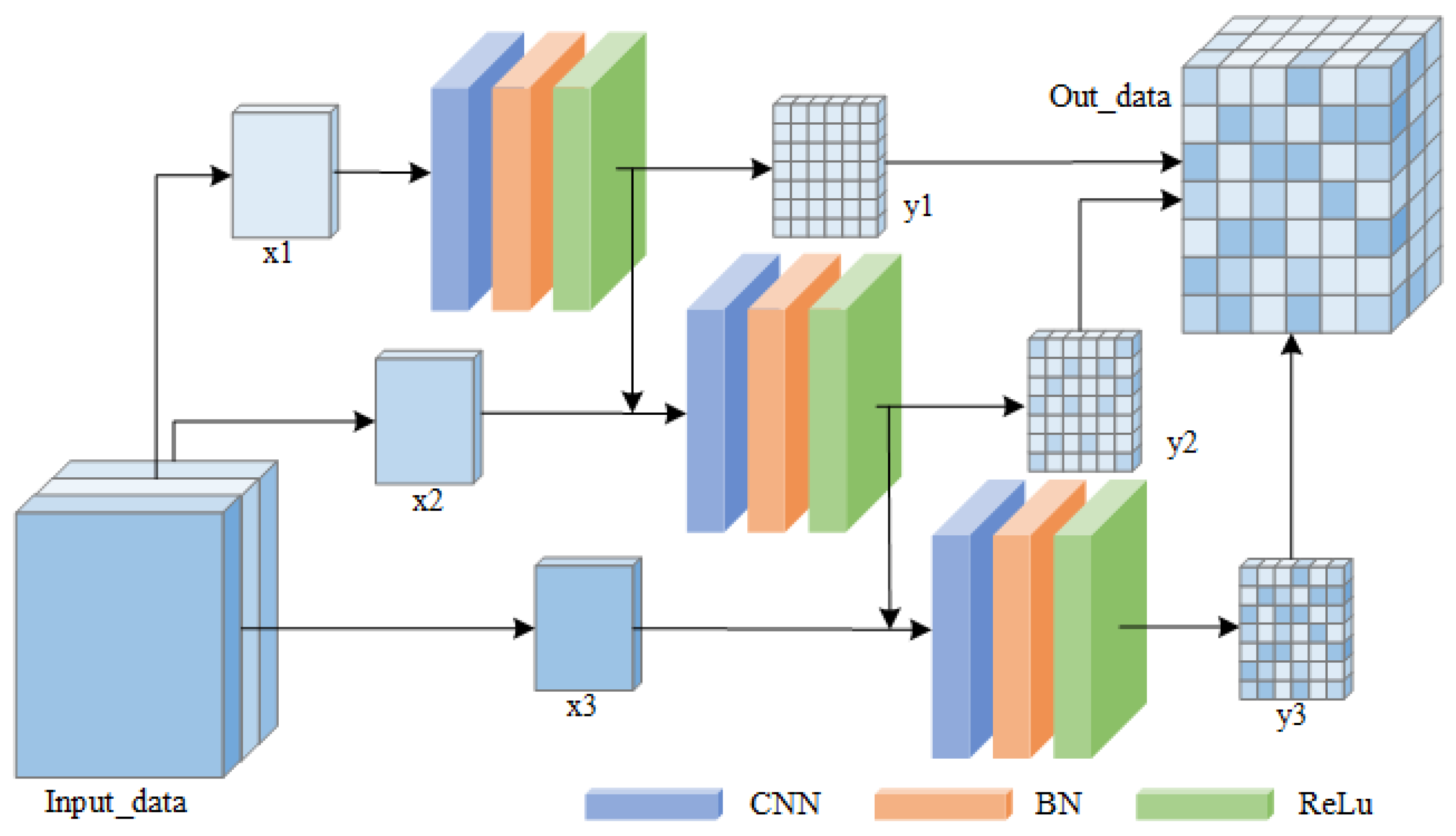
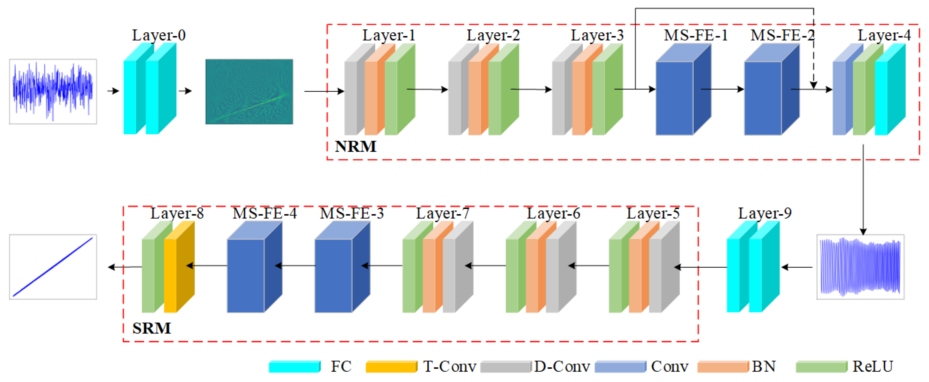
3.1. Design of HRRnet

The HRRnet proposed in this paper consists of two main parts, namely the noise reduction module (NRM) and the spectral representation module (SRM), as shown in Figure 5. The NRM is composed of the Dilated Convolution Layer (D-Conv) and the MS-FE. It is used to expand the receptive field, increase the diversity of feature extraction, and enhance the noise reduction ability of the network. The SRM is composed of the D-Conv, MS-FE, and Transposed Convolution Layer (T-Conv). Through the extraction of global and local features, it strengthens the expressiveness of the features. On this basis, the T-Conv is utilized to achieve a high-resolution representation of the time–frequency spectrum.

The HRRnet employs two FCs to transform one-dimensional time-domain signals into two-dimensional time–frequency signals. Subsequently, the NRM utilizes three layers of D-Conv to expand the receptive field of the network for signals. Meanwhile, it maps the signals to a high-dimensional space to extract global features and sets appropriate DR coefficients to prevent the loss of local information. Then, in the high-dimensional space, two layers of MS-FE are used to extract multi-scale local features, and the fusion of global features and multi-scale local features is achieved in the high-dimensional space by means of shortcut connections. Finally, 1 × 1 convolution is adopted to reduce the dimensionality, and the FC is used to convert the signals into one-dimensional time-domain signals after noise reduction processing. The specific parameters of the NRM are shown in

Table 1. NRM parameters.

Layer Name	Output Dimension	Convolution Kernel Size	Convolution Rate
Input	2 × 512	-	-
Layer-0	32 × 32	-	-
Layer-1	32 × 32 × 32	3 × 3	1
Layer-2	32 × 32 × 32	3 × 3	2
Layer-3	64 × 32 × 32	3 × 3	5
MS-FE-3	64 × 32 × 32	1 × 1/3 × 3	1
MS-FE-4	64 × 32 × 32	1 × 1/3 × 3	1
Layer-4	2 × 512	1 × 1	1

.

The HRRnet utilizes two FCs to convert the time-domain signals that have undergone noise reduction processing into two-dimensional time–frequency domain signals with low resolution. After that, the SRM employs three layers of D-Conv and two layers of MS-FE in the time–frequency domain to complete the extraction of global features and local multi-scale features. Finally, T-Conv is used to perform the upsampling operation to expand the data size to 5120, thereby achieving the purpose of improving the resolution and enhancing the estimation accuracy. The specific parameters of the SRM are shown in

Table 2. SRM parameters.

Layer Name	Output Dimension	Convolution Kernel Size	Convolution Rate
Layer-9	32 × 32 × 32	-	-
Layer-5	32 × 32 × 32	3 × 3	1
Layer-6	32 × 32 × 32	3 × 3	2
Layer-7	64 × 32 × 32	3 × 3	5
MS-FE-3	64 × 32 × 32	1 × 1/3 × 3	1
MS-FE-4	64 × 32 × 32	1 × 1/3 × 3	1
Layer-8	1 × 5120	3 × 3	1

.

In order to reduce the impact of burst noise on the performance of HRRnet, BN and ReLU are added between each layer. They are used to limit the range of the output data, achieve data decoupling between layers in the network, and thus accelerate the convergence speed of network parameters.

3.2. Parameter Optimization Algorithms for HRRnet

The parameter optimization algorithms pertaining to HRRnet encompass the algorithm for optimizing the parameters of the noise reduction module as well as that for the spectral line representation module. The computational procedure of the parameter optimization algorithm within the noise reduction module is illustrated in Equations (8)–(10).

$$\widehat{X}=\mathrm{Nrm}({\omega }_n,Y)$$

(8)

$$Los{s}_n=\mathrm{MSE}(\widehat{X},X)$$

(9)

$${\omega }_n^{*}=\underset{{\omega }_n}{\mathrm{argmin}}\left(Los{s}_n\right)$$

(10)

In the equation, Y represents the received time-domain signal; Nrm(•) stands for the noise reduction operation; $\widehat{X}$ is the signal after noise reduction; ${\omega }_n$ refers to the parameters of the noise reduction module; and MSE(•) represents the mean square error operation. The noise reduction module realizes the update of ${\omega }_n$ by minimizing $Los{s}_n$, reduces the error between $\widehat{X}$ and the transmitted signal X, and obtains the optimal parameter ${\omega }_n^{*}$ of the noise reduction module, thus completing the noise reduction of the received signal.

The computational process of the parameter optimization algorithm for the spectral line representation module is shown in Equations (11)–(13).

$$\widehat{R}=Srm({\omega }_s,\widehat{X})$$

(11)

$$Los{s}_s=MSE(\widehat{R}\left(0\right),f_0)+MSE\left[{\displaystyle \frac{|\widehat{R}\left(t_1\right)-\widehat{R}\left(t_2\right)|}{d_t}},\mu \right]+\alpha MSE(\widehat{R},R)$$

(12)

$${\omega }_s^{*}=\underset{{\omega }_s}{\mathrm{argmin}}\left(Los{s}_s\right)$$

(13)

In the formula, R represents the high-resolution time–frequency spectrum of the signal and is used as the training label, while $\widehat{R}$ is the estimated value of R; Srm(•) stands for the high-resolution spectral line representation estimation operation. $\widehat{R}\left(t_1\right)$ and $\widehat{R}\left(t_2\right)$, respectively, denote the estimated values of the instantaneous frequencies at time $t_1$ and $t_2$. $d_t$ is the time interval between $t_1$ and $t_2$, that is, $d_t=|t_1-t_2|$, and $\alpha$ is a hyperparameter, which is set to 0.3. The SRM completes the update of ${\omega }_s$ by minimizing $Los{s}_s$; reduces the errors among $\widehat{R}$ and R, $\widehat{R}\left(0\right)$ and $f_0$, and ${\displaystyle \frac{|\widehat{R}\left(t_1\right)-\widehat{R}\left(t_2\right)|}{d_t}}$ and $\mu$; obtains the optimal weight ${\omega }_s^{*}$ of the spectral line representation module; realizes the high-resolution representation of the time–frequency spectrum; and then achieves accurate estimations of the initial frequency $f_0$ and the frequency modulation coefficient $\mu$.

4. Simulation Verification and Analysis

4.1. Simulation Parameters

Under the condition of Gaussian noise, the SNR ranges from −15 dB to 0 dB with an interval of 1 dB. The main parameters of the training/testing samples under a single SNR are shown in

Table 3. Training/testing configuration parameters.

The Number of Training/ Testing Samples	Initial Frequency (Hz)	Frequency Modulation Coefficient (Hz)	Sampling Point Count	Sampling Frequency (Hz)
3000/500	15∼20	5∼10	$2\times 512$	256

. The total number of training samples is 48,000. The initial frequency and the frequency modulation coefficient are uniformly selected at equal intervals of 0.05 Hz within the given ranges. The total number of testing samples is 8000, and the initial frequency and the frequency modulation coefficient are randomly selected at non-equal intervals within the given ranges.

Table 4. Network training parameters.

Optimizer	Learning Rate	Number of Training Epochs	Validation Method	Learning Rate Decay Strategy
Adam	0.001	100	10-fold cross-validation	0.8

shows the training parameters of the network. Among them, the learning rate decay strategy means that during the training process, when the loss function fails to decrease continuously for five times, the learning rate will be reduced to 0.8 times its original value.

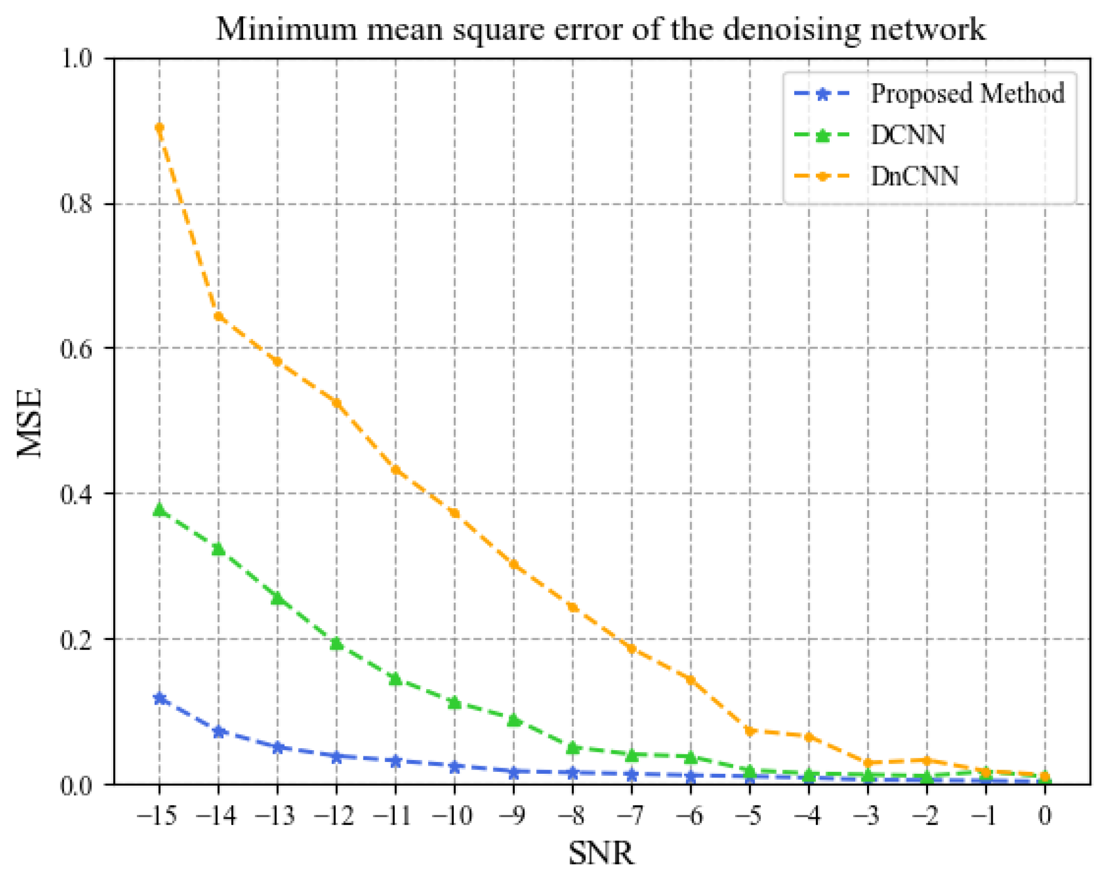
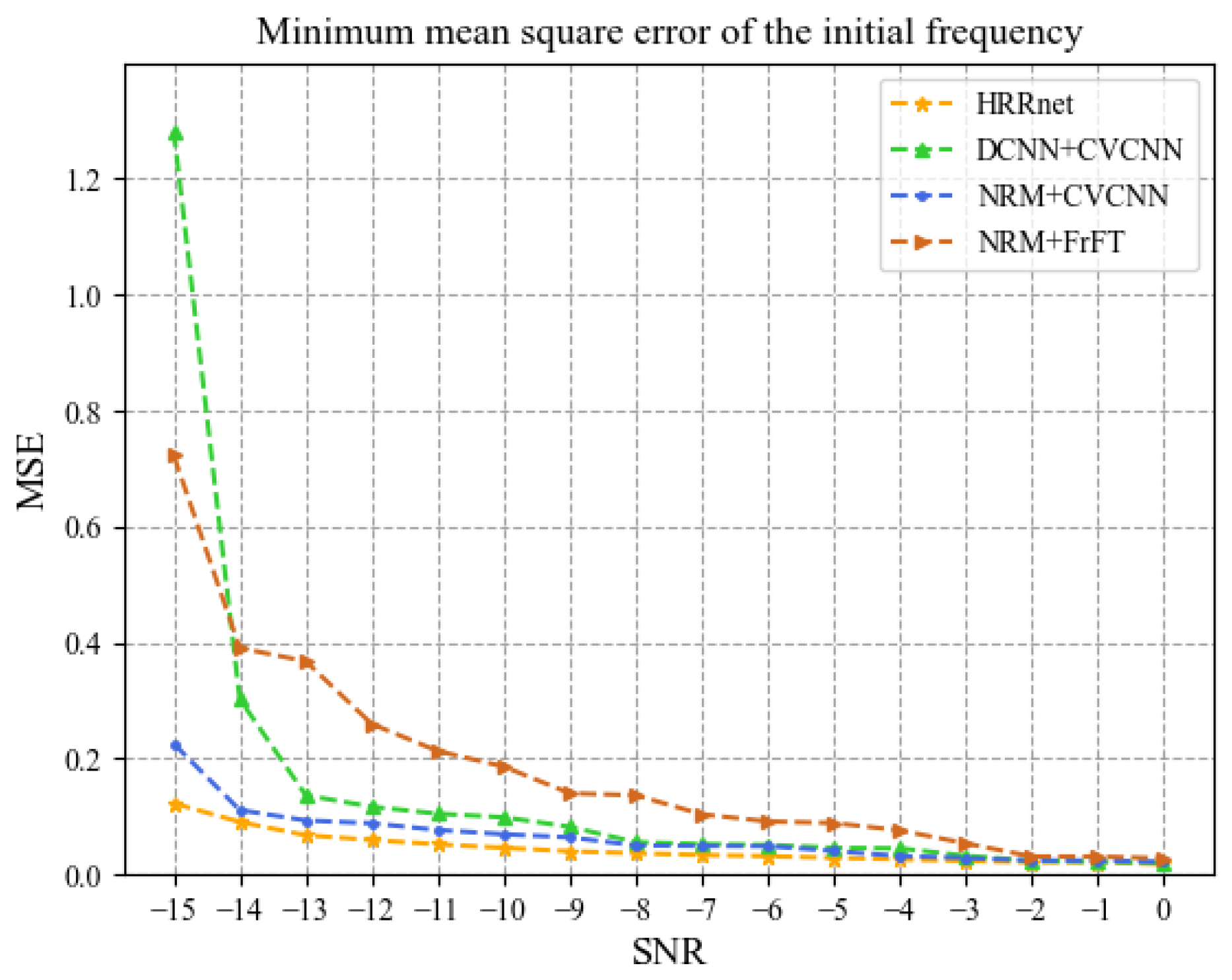
4.2. Analysis of Simulation Results

In this section, the performance of the method proposed in this paper is evaluated and verified from two aspects: noise reduction and parameter estimation. Under the same test conditions, DnCNN [21] and DCNN [18] are selected to compare the noise reduction performance with NRM.

Figure 6 presents the time–frequency diagrams of the signals after noise reduction using the above three methods when the SNR is −10 dB. Among them, (a) is the time–frequency diagram of the signal before noise reduction; (b) is the time–frequency diagram of the signal after noise reduction by DnCNN; (c) is the time–frequency diagram of the signal after noise reduction by DCNN; and (d) is the time–frequency diagram of the signal after noise reduction by NRM. It can be seen from the figure that all of the above methods can achieve noise reduction for the signals. By comparing the clarity of Figure 6b–d, it is obvious that NRM is significantly superior to the noise reduction methods of DnCNN and DCNN.

Figure 7 shows the comparison of the minimum mean square error (MSE) between the signals after noise reduction using the above three methods and the original signals under different SNRs. As shown in the figure, the MSE of NRM is lower than that of the other two noise reduction methods. Especially when $SNR\le -5$ dB, the mean values of the MSE of the NRM, DCNN, and DnCNN noise reduction methods are 0.037, 0.151, and 0.402, respectively, and the performance of the NRM method is significantly better than that of the other two methods.

The computational complexity and the number of parameters of NRM, DCNN, and DnCNN are shown in

Table 5. Network complexity.

Network Name	NRM	DCNN	DnCNN
Number of Parameters	4.21 M	4.35 M	4.37 M
Computational Complexity	122.66 M	183.9 M	198.97 M

. It can be seen from the table that the number of parameters of NRM is 4.21 M, which is lower than that of DCNN and DnCNN. The computational complexity of NRM is 122.66 M, much lower than that of the other two noise reduction methods. Through the above comparative analysis, it can be found that the noise reduction module constructed in this paper achieves a good noise reduction effect with relatively low network overhead, which further proves the effectiveness of using the method of expanding the receptive field and fusing multi-scale features to enhance the expressiveness of the inherent features of the signal.

The combinations of DCNN with CV-CNN [12], NRM with CV-CNN, and NRM with FrFT [24] are selected to conduct comparison and verification with HRRnet. Under the premise of noise reduction, parameter estimation of the LFM signals is achieved to ensure the objectivity and accuracy of the simulation verification.

$$ACC={\displaystyle \frac{N_{\left(\right|\partial -{\partial }^{\prime }|<\eta )}}{N_{\partial }}}\times 100\%$$

(14)

Equation (14) presents the calculation formula for the parameter estimation accuracy rate (ACC). Among them, $N_{\partial }$ represents the total number of test samples; ${\partial }^{\prime }$ is the estimated value of the parameter ∂. In this paper, ∂ represents the initial frequency or the frequency modulation coefficient; $\eta$ is the tolerable error; and $N_{\left(\right|\partial -{\partial }^{\prime }|<\eta )}$ represents the number of samples whose estimation deviation values are lower than $\eta$.

Figure 8 and Figure 9, respectively, show the estimation ACC of the initial frequency $f_0$ when $\eta$ = 0.1 and $\eta$ = 0.05. It can be seen from figures that the ACC of $f_0$ estimated by HRRnet is better than that of the other three methods. When the SNR is in the range of −12 dB to 0 dB and $\eta$ = 0.1, the average values of the ACC of HRRnet, NRM + CV-CNN, DCNN + CV-CNN, and NRM + FrFT are 95.53%, 87.25%, 84.1%, and 70.37% respectively. When $\eta$ = 0.05, the average value of the ACC of HRRnet is 75.86%, which is successively higher than that of the other three methods by 3.86%, 16.71%, and 20.82%. In addition, under the same conditions, the ACC of the NRM + CV-CNN method is higher than that of the DCNN + CV-CNN method, which further illustrates that the noise reduction ability of NRM is better than that of DCNN.

Figure 10 and Figure 11, respectively, show the estimation ACC of the frequency modulation coefficient when $\eta$ = 0.1 and $\eta$ = 0.05. It can be seen from the figures that the ACC of $\mu$ estimated by HRRnet is the best. When the SNR is in the range of −12 dB to 0 dB and $\eta$ = 0.1, the average value of the ACC of HRRnet is 91.19%, which is higher than that of the other three methods by 8.49%, 19.06%, and 29.88%, respectively. When $\eta$ = 0.05, the average value of the ACC is 66.63%, which is higher than that of the other three methods by 10.18%, 16.71%, and 27.55%, respectively.

Figure 12 and Figure 13, respectively, show the minimum mean square errors of the estimated values of the initial frequency and the LFM coefficient under different SNRs. It can be seen from the figures that when the SNR is in the range of −15 dB to 0 dB, the mean value of the minimum mean square error of the estimated value of the initial frequency by HRRnet is 0.045, and the error values of NRM + CV-CNN, NRM + FrFT, and DCNN + CV-CNN are 0.070, 0.183, and 0.172, respectively. The mean value of the minimum mean square error of the estimated value of the LFM coefficient by HRRnet is 0.058, and the error values of NRM + CV-CNN, NRM + FrFT, and DCNN + CV-CNN are 0.066, 0.325, and 0.155, respectively.

The number of parameters and computational complexity of HRRnet, NRM + CV-CNN, and DCNN + CV-CNN are shown in

Table 6. Network complexity.

Network Name	HRRnet	NRM + CV-CNN	DCNN + CV-CNN
Number of Parameters	56.81 M	277.33 M	277.47 M
Computational Complexity	246.05 M	1146.11 M	1207.35 M

. It can be seen from the table that the number of parameters and computational complexity of the HRRnet framework are significantly lower than those of the other two neural network-based parameter estimation methods. The number of parameters and computational complexity of NRM + CV-CNN and DCNN + CV-CNN are 4.87 times and 4.88 times, and 4.66 times and 4.91 times, those of HRRnet, respectively.

To sum up, under the conditions of different SNRs and different tolerable errors, the accuracy rates of HRRnet in estimating the initial frequency and the frequency modulation coefficient of the LFM signal are both higher than those of the other three methods, and its network overhead is the lowest. This result fully demonstrates that the parameter estimation method constructed based on the idea of high-resolution spectral line representation has practical feasibility and good effectiveness.

5. Conclusions

This paper proposes a high-resolution spectral line representation network named HRRnet to achieve the estimation of the parameters of LFM signals. Taking the optimization of receptive field expansion and multi-scale feature extraction and fusion as the design concepts, this network constructs a noise reduction module and a spectral line representation module, which are used to reduce noise interference and perform high-resolution representation of the time–frequency spectrum, and then realize the estimation of the parameters of LFM signals.

Under different SNRs, this paper verifies the noise reduction performance and parameter estimation performance of HRRnet. The simulation results show that under the same test conditions, HRRnet has superior noise reduction ability, higher parameter estimation accuracy, and lower network overhead. It is proven that HRRnet is an LFM signal parameter estimation network with high efficiency and high accuracy. However, although this research has made progress in the processing of LFM signals, there is still room for improvement. In the future, on the one hand, we plan to apply this neural network to actual radar monitoring systems to put the research results into practice. On the other hand, we will also focus on issues related to complex noise environments and the processing of multi-component radar signals, contributing to the development of high-performance radar systems.

References

1. Palmer, R.D.; Yeary, M.B.; Schvartzman, D.; Salazar-Cerreno, J.L.; Fulton, C.; McCord, M. Horus—A Fully Digital Polarimetric Phased Array Radar for Next-Generation Weather Observations. IEEE Trans. Radar Syst. 2023, 1, 96–117. [Google Scholar] [CrossRef]
2. Johannes, W.; Caris, M.; Stanko, S. 94 GHz Radar Used for Perimeter Surveillance with Wide Target Clarification. In Proceedings of the 2020 21st International Radar Symposium (IRS), Warsaw, Poland, 5–8 October 2020; pp. 15–18. [Google Scholar] [CrossRef]
3. Zhang, T.; Zeng, T.; Zhang, X. Synthetic Aperture Radar (SAR) Meets Deep Learning. Remote Sens. 2023, 15, 303. [Google Scholar] [CrossRef]
4. Bullecks, B.; Suresh, R.; Rengaswamy, R. Rapid impedance measurement using chirp signals for electrochemical system analysis. Comput. Chem. Eng. 2017, 106, 421–436. [Google Scholar] [CrossRef]
5. Czarnecki, K.; Moszynski, M. A novel method of local chirp-rate estimation of LFM chirp signals in the time-frequency domain. In Proceedings of the 2013 36th International Conference on Telecommunications and Signal Processing (TSP), Rome, Italy, 2–4 July 2013; pp. 704–708. [Google Scholar]
6. Akan, A.; Karabiber Cura, O. Time–frequency signal processing: Today and future. Digit. Signal Process. 2021, 119, 103216. [Google Scholar] [CrossRef]
7. Lu, L.; Ren, W.X.; Wang, S.D. Fractional Fourier transform: Time-frequency representation and structural instantaneous frequency identification. Mech. Syst. Signal Process. 2022, 178, 109305. [Google Scholar] [CrossRef]
8. Shi, J.; Zheng, J.; Liu, X.; Xiang, W.; Zhang, Q. Novel Short-Time Fractional Fourier Transform: Theory, Implementation, and Applications. IEEE Trans. Signal Process. 2020, 68, 3280–3295. [Google Scholar] [CrossRef]
9. Cao, W.; Yao, Z.; Xia, W.; Yan, S. Parameter Estimation of Linear Frequency Modulated Signals Based on Interpolated Short-Time Fractional Fourier Transform and Variable Weight Fitting. Acta Armam. 2020, 41, 9. [Google Scholar]
10. Sejdi, E.; Djurovi, I.; Stankovi, L. Fractional Fourier transform as a signal processing tool: An overview of recent developments. Signal Process. 2011, 91, 1351–1369. [Google Scholar] [CrossRef]
11. Wang, X.; Ying, T.; Tian, W. Spectrum Representation Based on STFT. In Proceedings of the 2020 13th International Congress on Image and Signal Processing, BioMedical Engineering and Informatics (CISP-BMEI), Chengdu, China, 17–19 October 2020; pp. 435–438. [Google Scholar] [CrossRef]
12. Brynolfsson, J.; Sandsten, M. Classification of one-dimensional non-stationary signals using the Wigner–Ville distribution in convolutional neural networks. In Proceedings of the 2017 25th European Signal Processing Conference (EUSIPCO), Kos, Greece, 28 August–2 September 2017; pp. 326–330. [Google Scholar]
13. Chen, J.Y.; Li, B.Z. The short-time Wigner–Ville distribution. Signal Process. 2024, 219, 109402. [Google Scholar] [CrossRef]
14. Guo, F.; Yang, L.; Zhang, Z. Fast algorithm for Radon-ambiguity transform. IET Radar Sonar Navig. 2015, 10, 553–559. [Google Scholar] [CrossRef]
15. Liu, F.; Sun, D.P.; Huang, Y.; Tao, R.; Wang, Y. Fast Parameter-Estimation of LFM Signal Based on Improved Combined WVD and Randomized Hough Transform. Acta Armam. 2009, 30, 1642–1646. [Google Scholar]
16. Feng, J.; Wu, Y.; Sun, H.; Zhang, S.; Liu, D. Panther: Practical Secure Two-Party Neural Network Inference. IEEE Trans. Inf. Forensics Secur. 2025, 20, 1149–1162. [Google Scholar] [CrossRef]
17. Chen, X.; Jiang, Q.; Su, N.; Chen, B.; Guan, J. LFM signal detection and estimation based on deep convolutional neural network. In Proceedings of the 2019 Asia-Pacific Signal and Information Processing Association Annual Summit and Conference (APSIPA ASC), Lanzhou, China, 18–21 November 2019; pp. 753–758. [Google Scholar]
18. Ben, G.; Zheng, X.; Wang, Y.; Zhang, X.; Zhang, N. Chirp Signal Denoising Based on Convolution Neural Network. Circuits Syst. Signal Process. 2021, 40, 5468–5482. [Google Scholar] [CrossRef]
19. Su, H.; Bao, Q. Deep Learning Enabled Parameters Estimation Using Time-Frequency Analysis of Chirp Signals. In Proceedings of the 2020 IEEE 5th International Conference on Signal and Image Processing (ICSIP), Nanjing, China, 23–25 October 2020; IEEE: New York, NY, USA, 2020. [Google Scholar] [CrossRef]
20. Jiang, Y.; Li, H.; Rangaswamy, M. Deep Learning Denoising Based Line Spectral Estimation. IEEE Signal Process. Lett. 2019, 26, 1573–1577. [Google Scholar] [CrossRef]
21. Zhang, K.; Zuo, W.; Chen, Y.; Meng, D.; Zhang, L. Beyond a Gaussian denoiser: Residual learning of deep CNN for image denoising. IEEE Trans. Image Process. 2016, 26, 3142–3155. [Google Scholar] [CrossRef] [PubMed]
22. Zou, H.; Lan, R.; Zhong, Y.; Liu, Z.; Luo, X. EDCNN: A novel network for image denoising. In Proceedings of the 2019 IEEE International Conference on Image Processing (ICIP), Taipei, Taiwan, 22–25 September 2019; pp. 1129–1133. [Google Scholar]
23. Gao, S.H.; Cheng, M.M.; Zhao, K.; Zhang, X.-Y.; Yang, M.-H.; Torr, P. Res2Net: A New Multi-Scale Backbone Architecture. IEEE Trans. Pattern Anal. Mach. Intell. 2021, 43, 652–662. [Google Scholar] [CrossRef] [PubMed]
24. Li, B.; Zhang, Z.; Zhu, X. Multitaper adaptive short-time Fourier transform with chirp-modulated Gaussian window and multitaper extracting transform. Digit. Signal Process. 2022, 126, 103472. [Google Scholar] [CrossRef]
Figure 1. LFM signal time–frequency representation diagram (SNR = 0 dB; SNR = −10 dB).
Electronics 14 01121 g001
Figure 2. Traditional neural network structure diagram.The solid line arrows represent direct connections, while the dashed line arrows indicate omissions.
Electronics 14 01121 g002
Figure 3. MS-FE structure diagram.The various colors in the figure represent the characteristics of different channels.
Electronics 14 01121 g003
Figure 4. Time–frequency spectral line diagram of LFM signal.
Electronics 14 01121 g004
Figure 5. HRRnet frame structure diagram. The color boxes are used to represent different network layer components in the HRRnet framework structure. The solid line arrows represent direct connections, while the dashed line arrows indicate omissions.
Electronics 14 01121 g005
Figure 6. Comparison of noise reduction time–frequency maps.
Electronics 14 01121 g006
Figure 7. Comparison of minimum mean square error.
Electronics 14 01121 g007
Figure 8. Initial frequency estimation accuracy ( η = 0.1).
Electronics 14 01121 g008
Figure 9. Initial frequency estimation accuracy ( η = 0.05).
Electronics 14 01121 g009
Figure 10. Frequency modulation coefficient estimation accuracy ( η = 0.1).
Electronics 14 01121 g010
Figure 11. Frequency modulation coefficient estimation accuracy ( η = 0.05).
Electronics 14 01121 g011
Figure 12. Minimum mean square error of initial frequency.
Electronics 14 01121 g012
Figure 13. Minimum mean square error of frequency modulation coefficient.
Electronics 14 01121 g013