4D Track Prediction Based on BP Neural Network Optimized by Improved Sparrow Algorithm

Abstract

The prediction accuracy of 4D (four-dimensional) trajectory is crucial for aviation safety and air traffic management. Firstly, the sine chaotic mapping is employed to enhance the sparrow search algorithm (Sine-SSA). This enhanced algorithm optimizes the threshold parameters of the BP (back propagation) neural network (Sine-SSA-BP), thereby improving the quality of the initial solution and enhancing global search capability. Secondly, the optimal weight thresholds obtained from the Sine-SSA algorithm are integrated into the BP neural network to boost its performance. Subsequently, the 4D trajectory data of the aircraft serve as input variables for the Sine-SSA-BP prediction model to conduct trajectory predictions. Finally, the prediction results from three models are compared against the actual aircraft trajectory. It is found that within the specified time series, the errors in longitude, latitude, and altitude for the Sine-SSA-BP prediction model are significantly smaller than those of the simple BP and SSA-BP models. This indicates that the Sine-SSA-BP model can achieve high-precision 4D trajectory prediction. The accuracy of trajectory prediction is notably improved by the sparrow search algorithm optimized with sine chaotic mapping, leading to faster convergence and better prediction outcomes, which better meet the requirements of aviation safety and control.

1. Introduction

The 4D trajectory encompasses the motion state of an aircraft in the air in latitude, longitude, height, and time, representing classical time-series correlated data. [1]. Four-dimensional trajectory prediction technology will be the core technology of air traffic management automation systems in the future and it is also an important component of civil aviation TBO (trajectory-based operation) plate. Judith Rosenow et al. (2017) demonstrated the positive impact of 4D-optimized trajectories on the air traffic flow, controller’s task load, and airspace complexity and emphasize the importance of an enhanced air traffic flow management considering dynamic sectorization and airspace [2]. There is a parameter-free method based on the Kalman filter or neural network estimation algorithm, which has a small amount of data and simple calculation. Ma Lan and Tian Shan (2020) put forward the aircraft maneuver mode using strategy and introduced the high-altitude wind information from weather information into the aircraft 4D model to optimize the aircraft 4D trajectory calculation model [3]. Tastamberkov, et al. (2014) combined the idea of “regression” in traditional mathematics with aircraft trajectory prediction and utilized mathematical methods such as multiple logistic regression and wavelet decomposition to integrate with machine learning model systems, effectively realizing the regression concept of aircraft trajectory prediction [4]. Jiang, S.-Y. et al. (2021) addressed the issues of low computational efficiency and prediction accuracy of optimization models by obtaining flight intentions and strategies coupled with weather information for trajectory prediction optimization [5]. Baek, K. and Bang, H. (2012) proposed an efficient and accurate algorithm to calculate conflict probability using ADS-B data by approximating the conflict zone with a set of blocks [6]. Gallego, C.E.V. et al. (2019) developed a probabilistic horizontal interdependency measure between aircraft supported by machine learning algorithms that can identify associated air traffic control actions upon them and their impact on the vertical profile of the trajectories [7]. Liu, Z. et al. (2020) presented a deep neural network-based online trajectory generation method for the aerodynamic characteristic description and terminal-area energy management of wave-rider aircrafts [8]. Pham, J. et al. (2019) predicted real-time 3D deformation field maps (DFMs) using Volumetric Cine MRI (VC-MRI) and adaptive boosting and multilayer perceptron neural network (ADMLP-NN) for 4D target tracking [9]. Xu, Z.F. et al. (2023) proposed a 4D trajectory prediction model of a social spatiotemporal graph convolutional neural network (S-STGCNN) based on pattern matching [10]. The traditional BP (back propagation) neural network model has the problem of low accuracy in 4D track prediction, while the swarm intelligence optimization algorithm seeks the global optimal solution, which can greatly improve the accuracy of track prediction [11]. This paper proposes optimizing the BP neural network based on the swarm intelligence optimization algorithm to explore the change rule between track and actual time and space. The sparrow search algorithm (SSA) is a relatively new swarm intelligence algorithm. It is mainly inspired by the feeding behavior of sparrows. It has strong global optimization ability, good parallelism, and fast convergence. Compared to other swarm intelligence optimization algorithms, it has better convergence accuracy, speed, and stability [12]. In this study, we train the obtained data through a BP neural network, initialize the sparrow population, and place it into the trained network for further updates to optimize the network’s weight threshold. Additionally, sine chaotic mapping expands the search range to better locate the global optimal solution. Experimental results demonstrate the effectiveness and superiority of the proposed 4D trajectory prediction method, enhancing trajectory prediction accuracy.

2. Sparrow Search Algorithm

The sparrow search algorithm (SSA) [13], proposed in 2020, is a swarm intelligence optimization algorithm inspired by the foraging behavior of sparrow populations. In SSA [14], each individual can be divided into discoverer, participant, and alerter. The discoverer is responsible for finding food and leading the population search. Participants follow the discoverer to snatch food. Alerters remain alert to environmental threats and warn sparrow populations to move to safe areas. When the finder does not find the threat (R₂ < ST), they are responsible for guiding the population foraging and conducting extensive searches. When an individual in a population detects a predator (natural enemy) and issues an alert (R₂ ≥ ST), it directs the population to a safe area. The location update is described as follows:

$$X_{i,j}^{t+1}=\left\{\begin{array}{ll}{X}_{i,j}^t·\exp \left({\displaystyle \frac{-i}{a·N}}\right)& \hfill R_2<ST\\ X_{i,j}^t+Q·L& \hfill R_2\ge ST\end{array}\right.$$

(1)

t represents the current iteration count, while N is a predefined constant that specifies the maximum number of iterations. $X_{i,j}$ indicates the positional information of the i-th sparrow in the j-th dimension. ɑ is a random number belonging to 0~1, Q is responsible for controlling the step size, and the step size is random. L is 1 × d, d denotes the size, and all elements are 1. The warning value R₂ is in the range of [0, 1] and the safety value ST is in the range of [0.5, 1]. In order to obtain food, participants followed and supervised the discoverer to grab food (i ≤ N/2) or find food alone (i > N/2). Therefore, the participant’s location update is described as follows:

$$X_{i,j}^{t+1}=\left\{\begin{array}{ll}Q·\exp \left({\displaystyle \frac{{X^t}_{Wp}-X_{i,j}^t}{i^2}}\right)& i>n/2\\ X_{i,j}^{t+1}+\left|X_{i,j}^t-X_p^{t+1}\right|·A^{+}·L& \mathrm{other}\end{array}\right.$$

(2)

X_Wp represents the worst position of the current population and X_p represents the best position currently occupied by the current discoverer. A is responsible for controlling the direction of the 1 × d matrix, the element is only 1 or −1, and A⁺ = A^T(AA^T)⁻¹. When aware of the danger, the sparrow population will make anti-predation behavior. The current fitness is greater than the fitness of the optimal position, indicating that the alerter is aware of the danger of the current position and they will approach other sparrows to reduce the risk of predation; when the current fitness is equal to the optimal position fitness, it means that the sparrow is on the edge of the population and the risk of attack by the predator is very high. In other cases, the joiner will follow the current finder in the vicinity of the optimal location foraging. The alarm location update formula is as follows:

$$X_{i,j}^{t+1}=\left\{\begin{array}{ll}{X}_{Bp}^t+\beta ·\left|X_{i,j}^t-X_{Bp}^t\right|& f_i>f_{Wp}\\ X_{i,j}^t+K·\left({\displaystyle \frac{X_{i,j}^t-X_{Wp}^t}{\left(f_i-fWp\right)+\epsilon }}\right)& f_i=f_{Bp}\end{array}\right.$$

(3)

β, as a step size control parameter, is a random number that follows a normal distribution with a mean of 0 and a variance of 1. $K\in [-1,1]$ is a random number. From the above mathematical expression, it is not difficult to see that with the change of the fitness value of the sparrow, as the population updates, the same sparrow may play three roles. As the discoverer, the sparrow has high energy. After the alerter detects the danger, the sparrows may evacuate to other safe areas. Due to the different flight trajectories, the followers with lower energy values are the first to evacuate to the safe area to feed and replenish energy to a certain value and play the discoverer to continue to find food. Therefore, each sparrow will change its role because of the warning signal. Finally, after a continuous iterative update, the global optimal value and the best fitness value are obtained.

3. Sine-SSA-BP Algorithm

The BP neural network possesses adaptive and nonlinear characteristics [15], which can address complex nonlinear problems and adapt to intricate input–output relationships. Therefore, it has been widely used in the field of track prediction. However, the BP neural network can be significantly influenced by the choice of learning rate due to its gradient correction, resulting in its slow convergence speed or oscillation [16]. Unknown disturbances and model selection can adversely affect the prediction accuracy of the neural network. The sparrow algorithm is an algorithm that adaptively adjusts the search parameters. It can automatically adjust the neural network parameters to improve the performance of the neural network [17]. The core concept of this algorithm involves refining the neural network’s output to align more closely with expected results through appropriate parameter adjustments. This process can be conceptualized as a “search” within the parameter space of the neural network, continuously seeking the optimal parameter combination based on the adjustment outcomes. The sparrow algorithm is a very effective neural network adjustment algorithm, which can achieve higher expected convergence accuracy to obtain better weights and thresholds, adapt to adjust neural network parameters, and improve the performance of neural networks. The sparrow algorithm is an optimization algorithm based on evolutionary computation. It can rapidly and efficiently adjust the neural network parameters, thus enhancing the model’s prediction accuracy.

Suppose that the matrix representation of the sparrow population is as follows, where n is the number of sparrows and d is the dimension of the variable:

$$X=\left[\begin{array}{cccc}{x}_{1,1}& x_{1,2}& \dots & x_{1,d}\\ x_{2,1}& x_{2,2}& \dots & x_{2,d}\\ ⋮& ⋮& \ddots & ⋮\\ x_{n,1}& x_{n,2}& \dots & x_{n,d}\end{array}\right]$$

(4)

Then the fitness value of each sparrow in the population can be expressed as follows:

$$Fx=\left[\begin{array}{c}f\left(\left[\begin{array}{cccc}{x}_{1,1}& x_{1,2}& \dots & x_{1,d}\end{array}\right]\right)\\ f\left(\left[\begin{array}{cccc}{x}_{2,1}& x_{2,2}& \dots & x_{2,d}\end{array}\right]\right)\\ ⋮\\ f\left(\left[\begin{array}{cccc}{x}_{n,1}& x_{n,2}& \dots & x_{n,d}\end{array}\right]\right)\end{array}\right]$$

(5)

Suppose that the number of neurons in the input layer, hidden layer, and output layer of the BP neural network are M, I, and J, then the dimension d of the sparrow population can be expressed as follows:

$$d=M+M\times I+I+I\times J+J$$

(6)

The fitness function selects the calculation formula of the reference mean square error, which is the average value of the mean square error of the training set and the test set. The smaller the fitness value, the more accurate the training and the better the prediction accuracy of the model. Its expression is:

$$f=\left({\sum _{i=1}^{n1}\sum _{j=1}^J\left(\widehat{X}train-X_0\right)}^2/n_1+{{\displaystyle \sum _{i=1}^{n2}{\displaystyle \sum _{j=1}^J\left(\widehat{X}test-X_0\right)}}}^2/n_2\right)/2$$

(7)

$X_0, \widehat{X}train, \widehat{X}test$ represents the original data, the output of the training set, and the output of the test set. n₁ and n₂ represent the number of training sets and test sets.

The SSA-BP algorithm flow is shown in Figure 1.

The specific process is as follows:

(1)

The topology of the BP neural network is determined. The number of nodes in the input layer is four and the number of nodes in the output layer is four. The optimal hidden layer m of the network structure is found by the minimum mean square error of the training set.

(2)

The 4D track data are preprocessed.

(3)

The weight threshold of BP is initialized. The initial weight experience value is between $(-2.4/F, 2.4/F)$ or $(-3/\sqrt{F}, 3/\sqrt{F})$. F is the number of neurons linked to the weight input.

(4)

SSA calculates the population fitness and updates the optimal individual and selects the population fitness function.

(5)

The SSA algorithm is initiated and the population engages in foraging and antipredation behaviors, with individual positions being dynamically updated.

(6)

The foraging and antipredation behavior of the population are determined, updating the individual position. In the SSA rule, the position of the individual will change constantly because of the different roles played by the individual and the individual position will be updated to the Formulas (1)–(3).

(7)

The termination condition of the algorithm is judged. It is substituted for the maximum number of iterations or less than or equal to the set convergence accuracy. If satisfied, continue to the next step; if not satisfied, return to step (4).

(8)

The optimal weights and thresholds obtained by the algorithm are substituted into the BP correction update and the training and simulation prediction are carried out again.

The sparrow algorithm is random in the individual search process and has strong search ability. Additionally, during the search process, the search parameters can be adaptively adjusted to meet the solution requirements of various problems. However, a limitation of the sparrow algorithm’s convergence mechanism is that if the optimal solution’s position is far from the origin, the algorithm may become trapped in local optima, leading to diminished global search performance. In this study, we improve the traditional spar-row algorithm by generating a random population sequence. The discrete chaotic mapping method [18], referred to as Sine-SSA [19,20], which is consistent with the algorithm and the problem, is used to optimize the initial population of the sparrow algorithm. It accelerates the optimization efficiency, reduces the likelihood of falling into local optima under the same population size and iteration count, and enhances the quality of the algorithm’s solutions. The improved sparrow algorithm based on sinusoidal chaotic mapping improves the initial population enriches the random sequence generated [21], improves the overall fitness value of the population and the initial quality of the population, is conducive to the selection and generation of the population, and improves the global search ability of the SSA algorithm. The expression of sinusoidal chaotic map [22] is:

$$X_{i+1}={\displaystyle \frac{\mu }{4}}·\sin (\pi ·X_i)$$

(8)

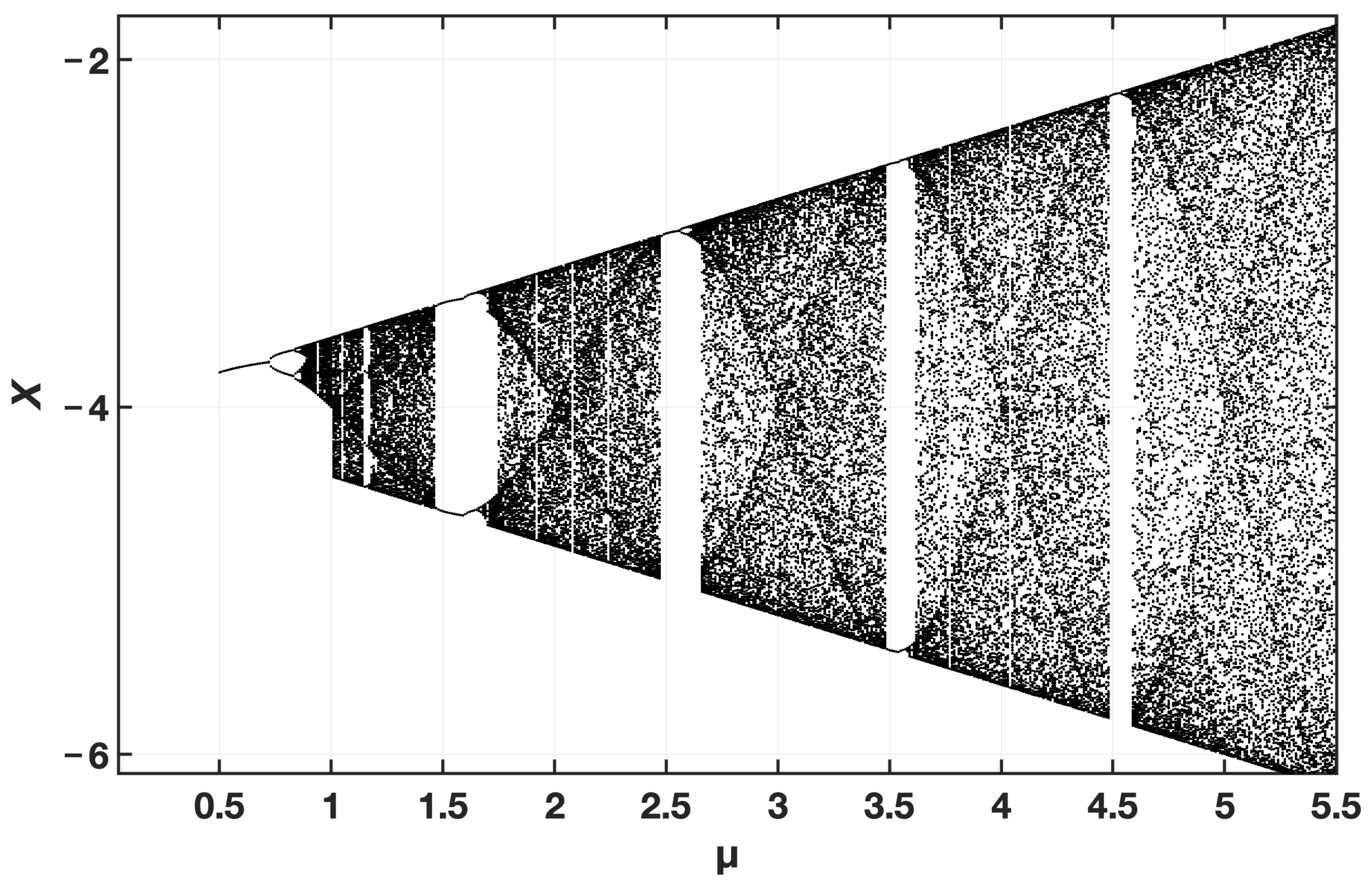
where μ is the control parameter in the range of [0, 4]. The sine chaotic map has obvious period-doubling bifurcation characteristics with many periodic windows, and its chaotic parameter interval is discontinuous. The sine map is distributed between [0, 1] and its chaos can replace random initialization, which can make the population more uniformly distributed in the search space. It is these characteristics that make the pseudorandom sequence generated by sinusoidal chaotic map more suitable for random requirements. The bifurcation diagram of the sine chaotic mapping is shown in Figure 2.

The chaotic sequence X generated by Equation (8) is used to obtain the sequence $X_{dim}$ with the best fitness:

$$X_{dim}=X_{f_{best}}$$

(9)

$f_{best}$ represents the highest fitness value. The initial population obtained by sine chaotic mapping is used as the initial population of the SSA algorithm, which enriches the diversity of the population, improves the overall fitness value of the population and the initial quality of the population, and improves the global search ability of the SSA algorithm. Therefore, this paper makes this algorithm an improved sparrow algorithm to optimize the BP neural network, referred to as Sine-SSA-BP. The specific process is shown in Figure 3.

The pseudo code of the Sine-SSA-BP algorithm is presented in Algorithm 1.

Algorithm 1 The Pseudocode of Sine-SSA-BP

begin Input the initial ADS-B data Output the prediction track set BP neural network parameters and structure net0=newff(inputdata,outputdata,hiddennum,{'tansig','purelin'},'trainlm'); net0=train(net0,inputdata,outputdata);%BP start training an0=sim(net0,inputtest);%BP forecast initial SSA parameters use Sine Chaotic mapping to initialize the position of population X0=sineInitialization;%The sine function initializes the population calculate initial fitness optimize parameters with SSA-foraging and antipredation behavior for i=1 to max generation   for j=1 to the numbers of finder     if Warning value< safety value       update the position of finder     else       not update     end   end   for j=the numbers of finder plus 1 to Population size     if j>the half of population       joiner find food by itself     else       update the position of joiner     end   end   for j=1 to the number of guard     if fitness>the best fitness       guard evacuate to safety place     elseif fitness=the best fitness       update the position of guard     end   end update positions update the weights and parameters of BP neural network net=train(net,input,output);%network training with new parameters an1=sim(net,input,out);%network forcasting

The primary parameters of the algorithm include:

• Population size, represented as an N × N matrix;
• Maximum evolution algebra, also known as the number of iterations;
• Safety value, which serves as the criterion for determining whether the discoverer’s position is updated according to Equation (1);
• Proportion of discoverers;
• Alert value, determined by Equation (3) to decide whether the alerter’s position is updated;
• Upper and lower limits of variables, essential for the proper implementation of the algorithm;
• Number of variables, determined by the number of neurons in the input layer, hidden layer, and output layer trained by the BP neural network, influencing the number of iterations within the algorithm.

Reasonable parameter settings are crucial for maximizing the algorithm’s performance and achieving optimal efficiency. For instance, the population size and the number of iterations directly impact the overall efficiency and runtime of the algorithm. The main parameter settings of the algorithm are summarized in

Table 1. The main parameter settings of the improved sparrow algorithm.

Network Parameter	Parameter Value
Popsize (number of initial populations)	30
Maxgen (maximum generation)	50
ST (safety value)	0.6
PD (proportion of discoverers)	0.7
SD (alert value)	0.2
Ub (upper limit)	3
Lb (lower limit)	−3
dim (dimension of the variable)	Calculated by Equation (6)

.

4. Experiments with ADS-B Data

The ADS-B system provides real-time and accurate monitoring information, such as the aircraft location [23], and has broad application prospects in air traffic services in high-density flight areas. The ADS-B data utilized in this study were obtained from the ADS-B receiving station of the Communication, Navigation, and Surveillance (CNS) Laboratory at the Civil Aviation Flight University of China. The receiving station uses a 1090ES data link with a coverage of 300 km. The ADS-B receiving subsystem comprises three functional modules: message reception, information conversion, and message generation. These modules are responsible for receiving, converting, and generating ADS-B messages. The system can receive S data link and other RF signals and output them to other airborne application subsystems after processing. The message receiving and conversion module includes receiving antenna and other RF signal processing equipment, while the message generation module is responsible for message conversion, message assembly, and output interface connected to the application layer. Subsequently, track prediction processing using the three algorithms was conducted in the MATLAB environment. The CNS laboratory ADS-B ground receiving equipment parameters are shown in

Table 2. The CNS laboratory ADS-B ground receiving equipment parameters.

Message Output Format	DF-17, DF-18, CAT-021
Information capacity	1500/s
Detection distance	350 km
Message output protocol	TCP
Communication interface	RJ45
1090 antenna interface	N type
GPS antenna interface	TNC
Power supply	28VDC 1A
Working environment	−20–55 °C

.

This dataset mainly includes aircraft arriving at and departing from Chengdu Shuangliu Airport as well as some aircraft passing through routes such as W230, G212, W233, and W81. The dataset spans a considerable time period and includes a large number of trajectories. The ground station is ADS-B standard signal format. Each dataset contains longitude (LON), latitude (LAT), time (TIME), GPS altitude (HEIGHT), barometric altitude (ALTITUDE), heading (HEADING), ground speed (GS), flight number (CALLSIGN), and other information. After decoding, this data can be utilized as a 4D trajectory prediction dataset. Data cleaning and interpolation were performed on the initially collected data and 11 flight datasets that met the specified criteria were selected. To evaluate the prediction performance of SSA and Sine-SSA after BP neural network optimization more objectively and comprehensively, this study selects datasets corresponding to five characteristic phases of flight: departure climb, cruise climb, cruise, cruise descent, and approach descent. The specific flights used for evaluation are CSC8843, CHB6335, CSN348, CSZ9238, and CSS6975.

4.1. Departure Climbing and Cruise Climbing

Due to potential signal blockage by obstacles, the ADS-B system in the laboratory generally cannot receive aircraft data at altitudes above approximately 4700 ft relative to Shuangliu Airport. Therefore, the process of an aircraft climbing from 4700 ft to 26,240 ft (approximately 8000 m) is defined as the off-site climbing stage. The subsequent climb from 8000 m to the designated cruise altitude is classified as the cruise climbing phase. Although the altitude changes during the cruise climbing phase, they are more gradual compared to the departure climbing phase due to the higher speed of the aircraft. In contrast, the altitude changes in the departure climbing phase are more frequent, which may affect the accuracy of altitude predictions. In this interval, the aircraft that meets the requirements is CSC8843 and the amount of data that meets the screening is 825. The training set is divided into 495 training sets for 8.25 min; the test set is 330 pieces for 5.5 min. Figure 4 and Figure 5 present a comparative analysis of the prediction outcomes and associated errors for four algorithms applied to the CSC8843 flight trajectory.

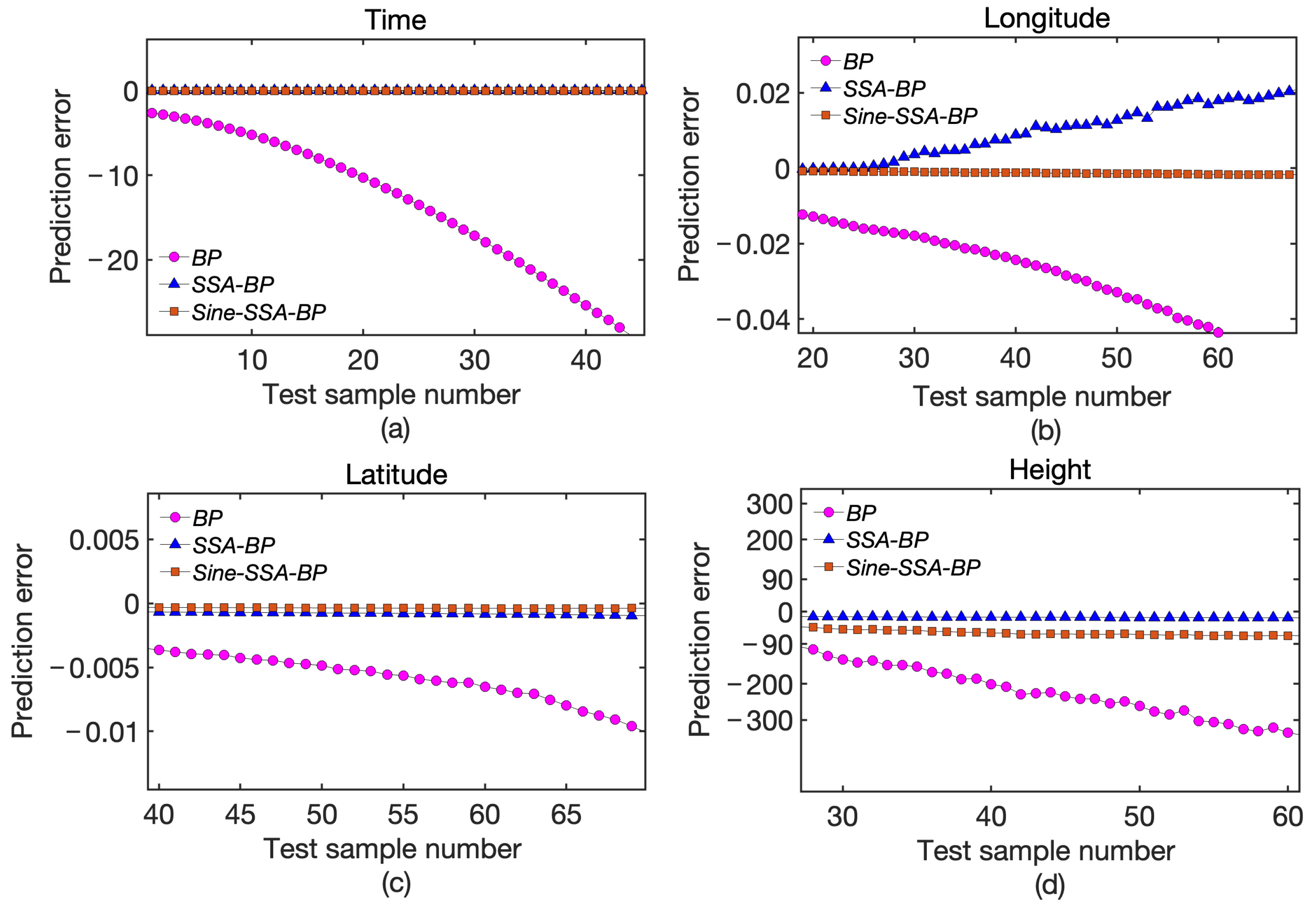
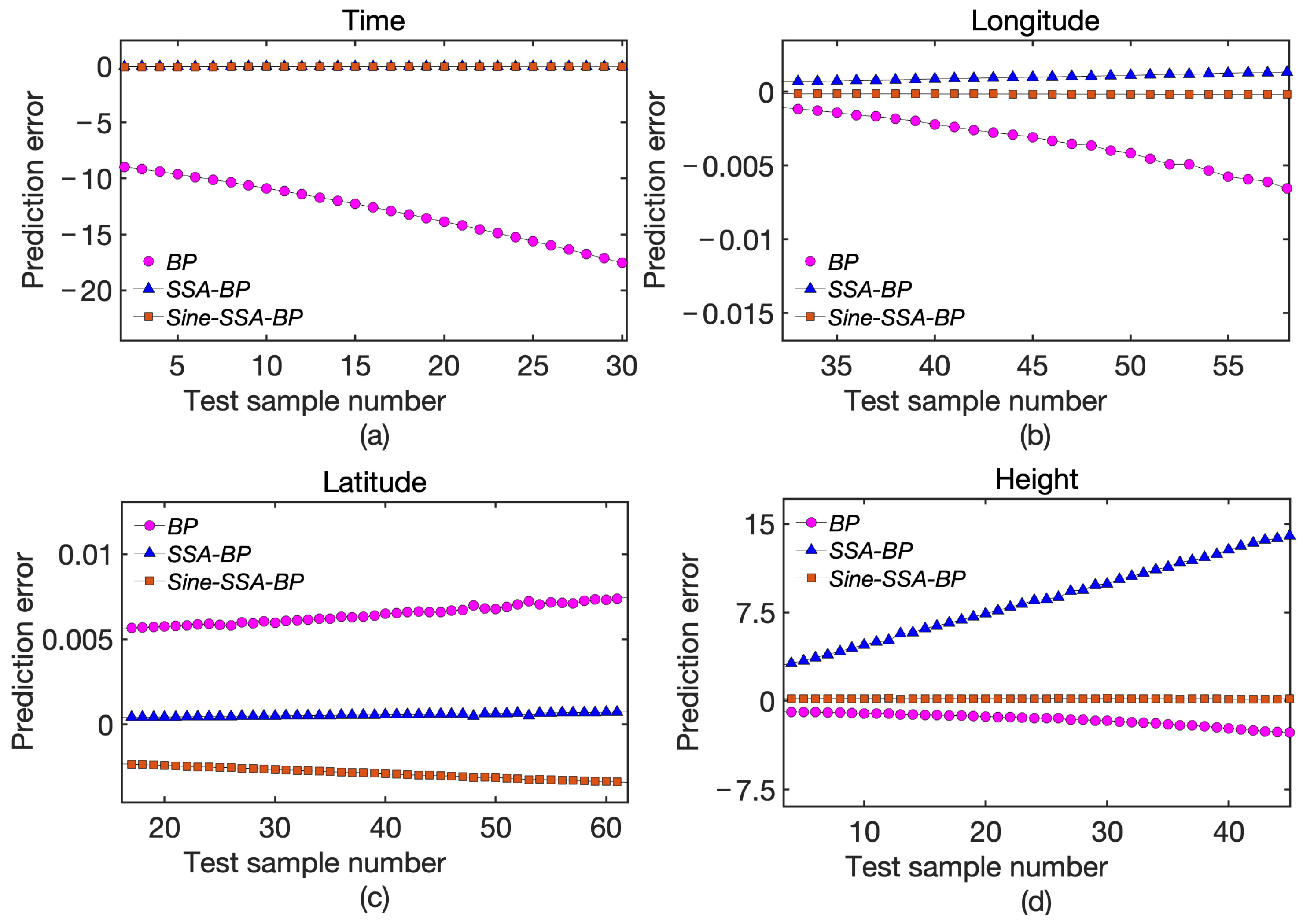
The results in Figure 4 demonstrate that the BP, SSA-BP, and Sine-SSA-BP algorithms exhibit high prediction accuracy in the early stages of the prediction sequence. However, as the prediction sequence progresses, the predicted values from the BP algorithm gradually deviate from the true values and approach the curve generated by the training function using the LM method, highlighting the limitations of the BP algorithm’s prediction capability with increasing data volume. Figure 5 shows that the deviation between the predicted and true values for SSA is relatively small but increases as the prediction sequence lengthens. Both the offsite climbing and cruise climbing phases are characterized by frequent changes in altitude. From the height prediction results obtained using the sparrow algorithm, there is almost no discernible difference between the predictions made by SSA and Sine-SSA and the true values. This indicates the effectiveness and applicability of the sparrow algorithm in predicting track height.

Figure 6 illustrates the prediction errors of various methods, clearly showing that the BP algorithm optimized by the sparrow algorithm exhibits significantly smaller errors compared to the standard BP algorithm. Specifically, the prediction accuracy for longitude and latitude has improved by more than an order of magnitude, while the accuracy for height has improved nearly two orders of magnitude. Additionally, the enhanced version of the sparrow algorithm has further improved performance, particularly in terms of latitude prediction, where accuracy has increased by approximately 20 times.

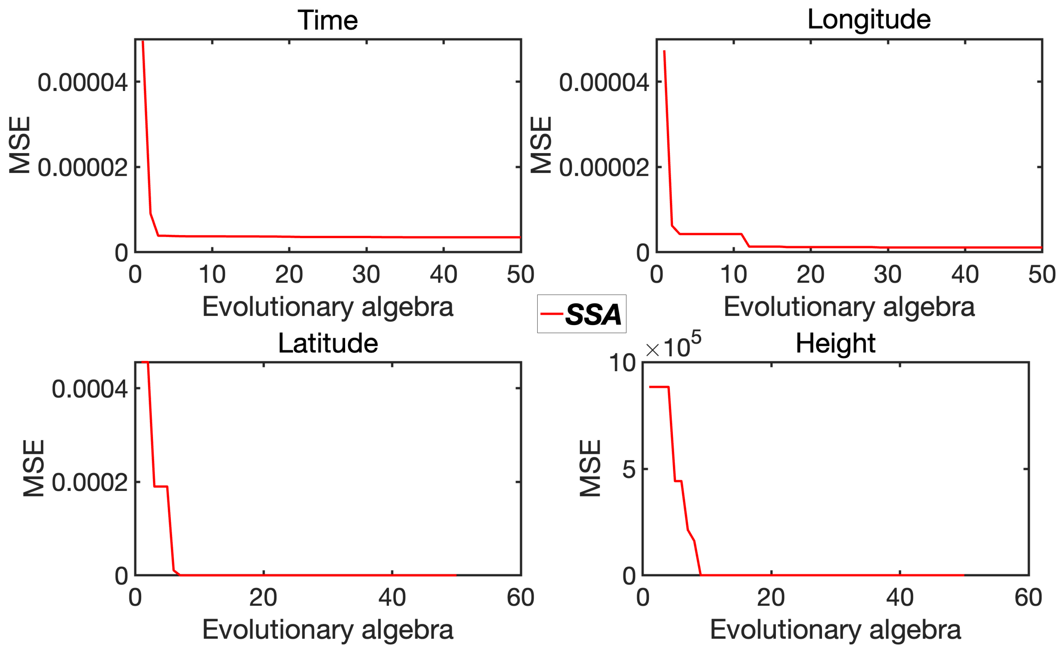
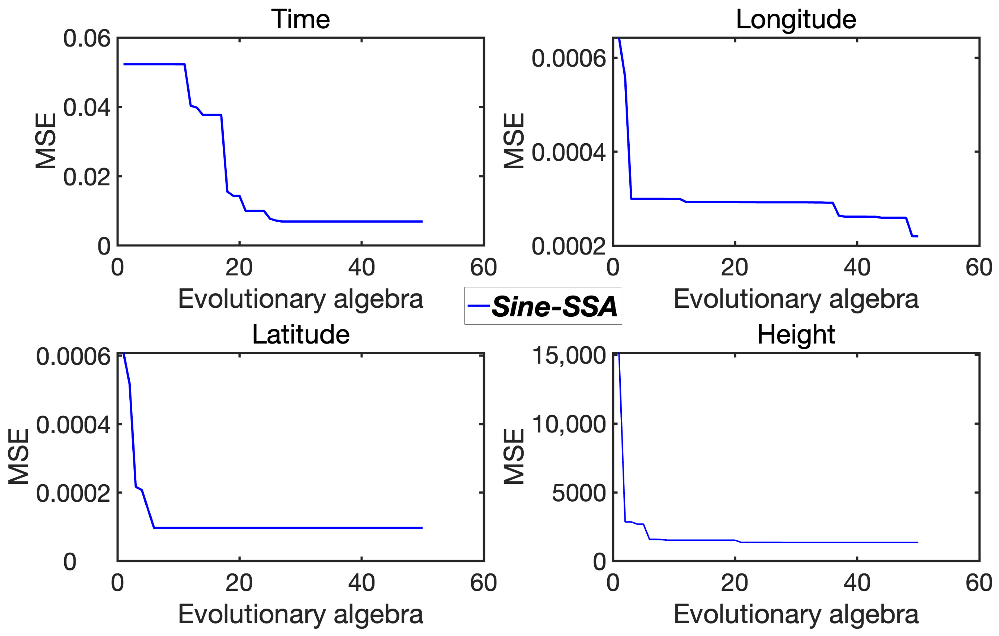
Figure 7 and Figure 8 depict the iterative convergence of each dimension for the sparrow algorithm (SSA) before and after improvement. It is evident that the convergence curve of the SSA (red) decreases rapidly, while the curve of the Sine-SSA (blue) compensates for both time and dimension. The original SSA exhibits slow convergence, whereas the Sine-SSA demonstrates faster convergence and a smaller mean square error, reflecting improvements in both accuracy and efficiency. The detailed error data are listed in

Table 3. CSC8843 track prediction error by different algorithms.

	Algorithm	MAE	MSE	RMSE	MAPE
Time	BP	149.81119	31,209.1945453	176.6612	0.210538
	SSA-BP	0.04742	0.0049932	0.0707	0.000068
	Sine-SSA-BP	0.00170	0.0000051	0.0023	0.000002
Longitude	BP	0.21650	0.0702382	0.2650	0.002058
	SSA-BP	0.01765	0.0004387	0.0209	0.000168
	Sine-SSA-BP	0.00112	0.0000016	0.0013	0.000011
Latitude	BP	0.12029	0.0240002	0.1549	0.003859
	SSA-BP	0.01008	0.0001943	0.0139	0.000323
	Sine-SSA-BP	0.00051	0.0000004	0.0006	0.000016
Height	BP	3169.3733	16,683,790.5253704	4084.5796	0.134937
	SSA-BP	42.22352	2663.6368545	51.6104	0.001833
	Sine-SSA-BP	27.16550	1339.4208888	36.5981	0.001371

.

In summary, the prediction accuracy can be quantified using the mean absolute percentage error (MAPE). By selecting the precise prediction segment (the first 10 data points) for calculation, the final prediction accuracy of the BP prediction model in the departure climb and cruise climb stages is 91.2%, that of the SSA-BP model is 99.4%, and that of the Sine-SSA-BP model is 99.6%.

4.2. Cruise

When the aircraft climbs above 8000 m, it can enter the cruising phase. However, due to the relatively low cruising altitude, cruising at this height is not economically optimal. Therefore, airlines typically set the cruising altitude within the RVSM airspace (8900 m to 12,500 m). The aircraft in this phase has a large number of points and complete data and can generally obtain data for more than 20 min. Moreover, the altitude of the aircraft entering the cruising altitude changes very little and the altitude change is mainly due to the influence of wind. In this study, flight CSN348 was selected as the aircraft that meets the specified criteria for this interval, with 2000 data points deemed eligible. The dataset is divided into a training set comprising 1200 data points covering 20 min and a test set consisting of 800 data points spanning 13.3 min. To illustrate the prediction performance and error characteristics of various algorithms across different dimensions, the results are depicted in Figure 9, Figure 10 and Figure 11.

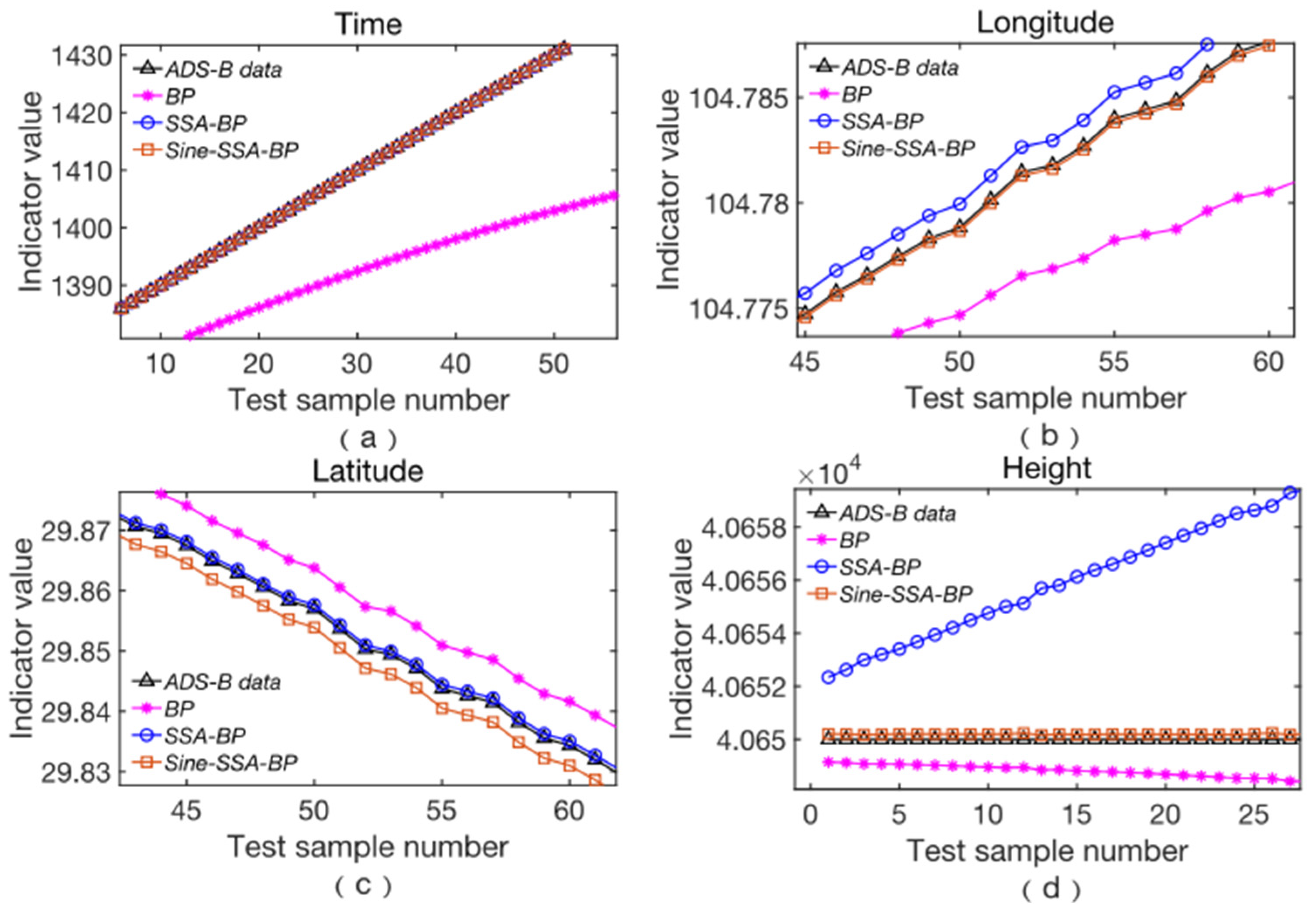
The data during the cruise phase are notably stable, leading to generally better prediction results compared to other flight phases. Figure 9 and Figure 10 illustrate the predictions of CSN348 in various dimensions. It is evident that the prediction accuracy of BP, SSA-BP, and Sine-SSA-BP has significantly improved compared to the departure climb stage. However, for longitude and altitude predictions, the BP algorithm still tends to follow the curve generated by the training function using the LM method. The sparrow algorithm exhibits a small deviation from the true values, with longitude remaining the dimension with the largest deviation. From the height prediction results obtained using the sparrow algorithm, it is clear that SSA-BP’s fitting to altitude is insufficient. In contrast, Sine-SSA-BP improves this by detecting changes as small as 10 feet, thereby refining altitude predictions. Figure 11 shows the prediction errors for the three methods applied to CSN348. The optimized BP algorithm demonstrates a significant reduction in error, while the enhanced sparrow algorithm further minimizes prediction errors.

Figure 12 and Figure 13 depict the iterative processes for the four dimensions after applying the two algorithms to predict the flight path of CSN348 during the cruise phase. Given that this is the cruise phase, changes in latitude and longitude are more pronounced. Consequently, the Sine-SSA algorithm can quickly converge and find the global optimal solution when predicting these dimensions. However, changes in altitude are less significant, requiring the Sine-SSA algorithm to undergo multiple iterations to escape local optima and identify the global optimal solution, thereby achieving higher prediction accuracy.

The deviation between the predictions of SSA and the true values remains relatively small, with longitude still exhibiting the largest deviation among all dimensions. From the height prediction results obtained using SSA, it is evident that SSA-BP has insufficient fitting for altitude. In contrast, Sine-SSA-BP improves this by detecting changes as small as 10 feet, thereby refining altitude predictions. The detailed error data are listed in

Table 4. CSN348 track prediction error by different algorithms.

	Algorithm	MAE	MSE	RMSE	MAPE
Time	BP	356.4150	177,668.4515062	421.5074	0.186812
	SSA-BP	1.13491	1.9757628	1.4056	0.000607
	Sine-SSA-BP	0.00017	0.0000000	0.0002	0.000000
Longitude	BP	0.28373	0.1174827	0.3428	0.002697
	SSA-BP	0.02394	0.0014988	0.0387	0.000227
	Sine-SSA-BP	0.07438	0.0116358	0.1079	0.000707
Latitude	BP	0.07802	0.0092105	0.0960	0.002715
	SSA-BP	0.00913	0.0001440	0.0120	0.000319
	Sine-SSA-BP	0.00787	0.0001104	0.0105	0.000273
Height	BP	163.66468	35,166.4710855	187.5273	0.004011
	SSA-BP	9.47823	132.4390239	11.5082	0.000233
	Sine-SSA-BP	0.58945	0.4828082	0.6948	0.000014

.

In summary, the prediction accuracy of the BP prediction model in the cruise phase is 95.1%, SSA-BP is 99.6%, and Sine SSA-BP is 99.7%.

4.3. Descent Approach and Cruise Descent

Due to the potential obstruction of ADS-B signals, this study defines the process of an aircraft descending from 26,240 ft (approximately 8000 m) to an altitude below 4700 ft as the descent and approach phase. The process of lowering the altitude from the cruise altitude to 8000 m is defined as the cruise descent phase. Contrary to the cruise climb phase, altitude changes during the cruise descent are relatively gradual, while those during the descent and approach phase are more frequent, potentially affecting the accuracy of altitude predictions.

In this interval, the flight that meets the specified criteria is CSS6975, with a total of 1079 data points deemed eligible. The dataset is divided into a training set comprising 648 data points covering 10.8 min and a test set consisting of 431 entries spanning 7.18 min. To illustrate the prediction performance and error characteristics of various algorithms across different dimensions, the results are depicted in Figure 14, Figure 15 and Figure 16.

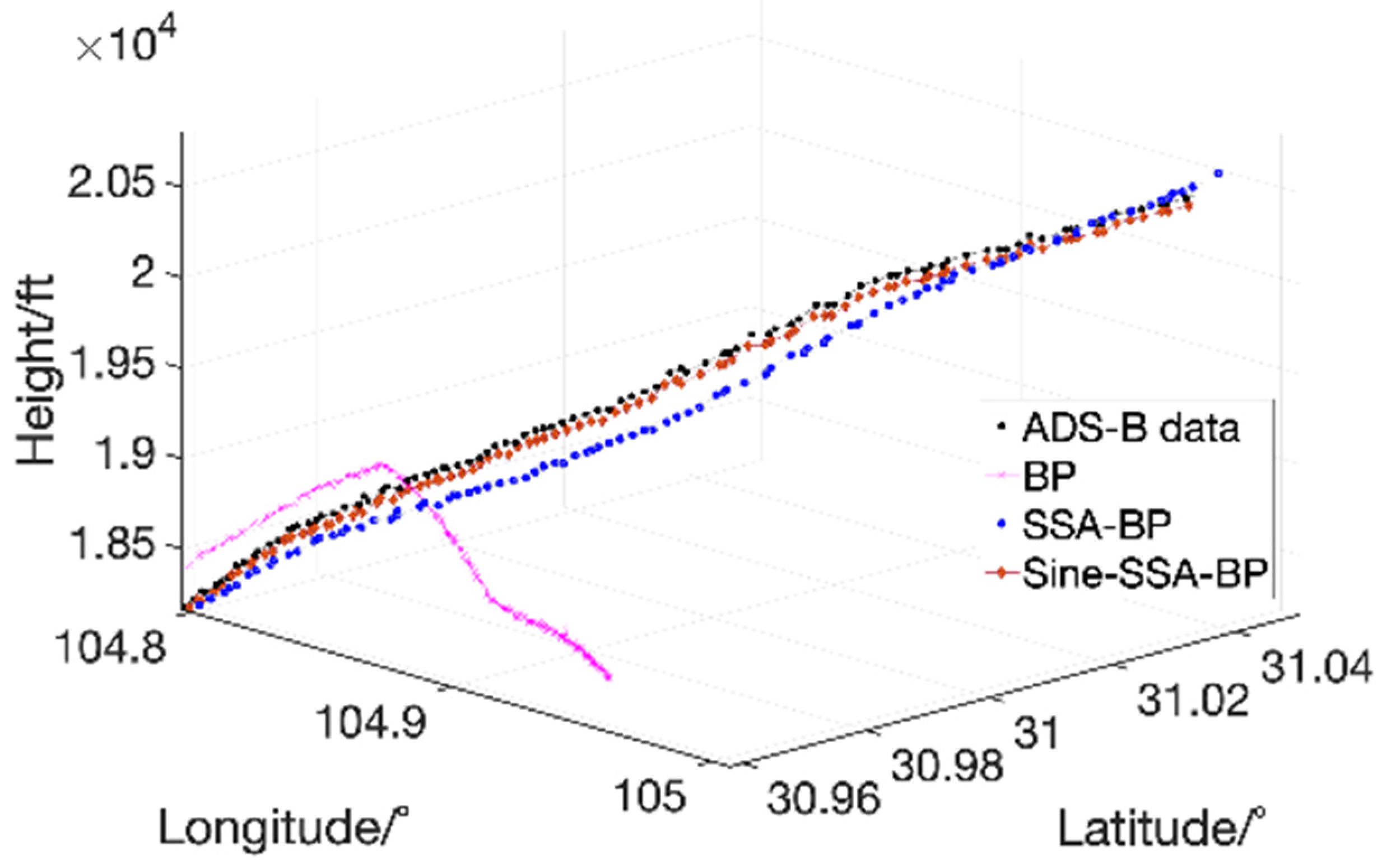
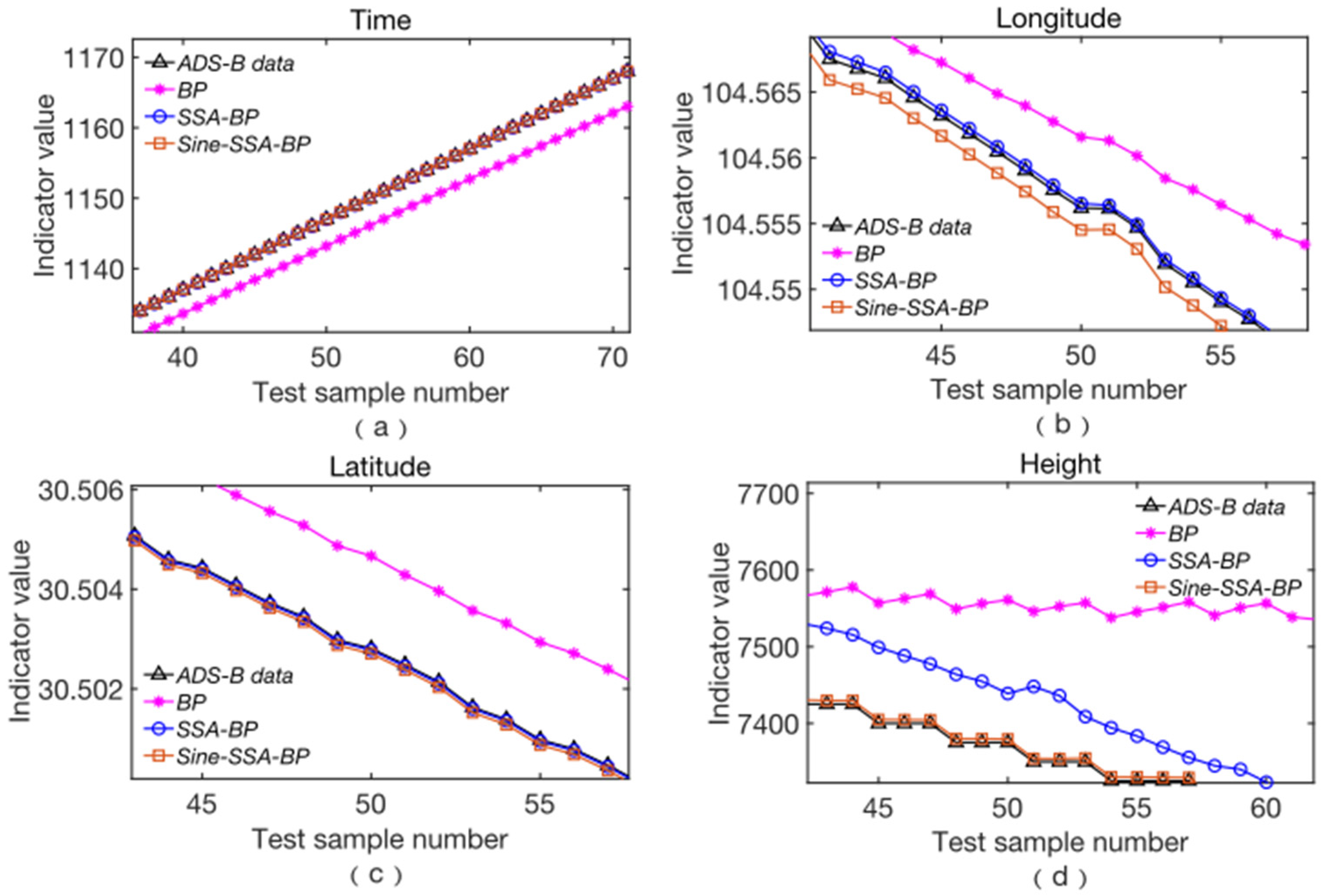
Figure 14 illustrates the prediction accuracy for each dimension during the descent and approach phase of flight CSS6975. Similar to the previous two phases, the prediction accuracy of BP, SSA-BP, and Sine-SSA-BP is high in the early stages of the prediction sequence. However, as the time series progresses, the prediction error of BP increases, approaching the curve generated by the training function using the LM method. In contrast, the deviation of the prediction of the sparrow algorithm from the true value is small, visually showing improvement after BP optimization, but its deviation increases as the prediction sequence increases. The departure climb and cruise climb phases are characterized by frequent changes in altitude. From the prediction results of the sparrow algorithm for height, the deviation of SSA and Sine-SSA from the true value is small, reflecting the applicability of the sparrow algorithm to predict the height of the flight path. The improved sparrow algorithm also shows significant enhancement compared to its preimprovement version.

Figure 15 illustrates the prediction errors for each method. It is evident that the error of the BP algorithm optimized by the sparrow algorithm is significantly smaller compared to the standard BP algorithm. Specifically, the prediction accuracy for longitude and latitude has improved by more than an order of magnitude, while the accuracy for height has improved nearly two orders of magnitude. Additionally, the enhanced version of the sparrow algorithm shows further improvements, particularly in latitude prediction, where accuracy has increased by approximately 20 times.

Figure 16 illustrates the comparison between track predictions and true values for four algorithms during the cruise descent phase of flight CSS6975. It is evident that in the early stages of prediction, there is no significant difference in the accuracy among the four methods. However, as the time series progresses, the BP algorithm becomes severely distorted. In contrast, SSA-BP and Sine-SSA-BP exhibit varying levels of accuracy in the later stages of the time series. Notably, SSA-BP shows a large deviation from the true ADS-B values in the later stages, while Sine-SSA-BP maintains a high degree of consistency with the true ADS-B values throughout the entire time series, demonstrating consistently high prediction accuracy.

Figure 17 and Figure 18 depict the iterative convergence of each dimension for the sparrow algorithm (SSA) before and after improvement. It is evident that the convergence curve of SSA (red) decreases rapidly, while the curve of Sine-SSA (blue) compensates for both time and dimensionality. The slower convergence of SSA and its higher mean square error highlight the improvements in accuracy and efficiency achieved by Sine-SSA. The detailed error data are listed in

Table 5. CSS6975 track prediction error by different algorithms.

	Algorithm	MAE	MSE	RMSE	MAPE
Time	BP	68.94177	9112.4301412	95.4590	0.048493
	SSA-BP	0.02897	0.0022299	0.0472	0.000021
	Sine-SSA-BP	0.00004	0.0000000	0.0000	0.000000
Longitude	BP	0.13285	0.0263737	0.1624	0.001275
	SSA-BP	0.00050	0.0000004	0.0006	0.000005
	Sine-SSA-BP	0.00325	0.0000146	0.0038	0.000031
Latitude	BP	0.02196	0.0010314	0.0321	0.000722
	SSA-BP	0.00083	0.0000015	0.0012	0.000027
	Sine-SSA-BP	0.00022	0.0000001	0.0003	0.000007
Height	BP	3590.52486	21,017,388.715	4584.47	0.646996
	SSA-BP	526.51471	355,144.640	595.9401	0.088499
	Sine-SSA-BP	6.06102	53.4573075	7.3115	0.000978

.

In summary, the prediction accuracy of the BP prediction model during the cruise descent phase is 82.6%, SSA-BP is 97.8%, and Sine-SSA-BP is 99.7%.

5. Discussion

The sparrow algorithm and the improved sparrow algorithm proposed in this study have significantly enhanced the accuracy of trajectory prediction, with acceptable prediction results for specific sequence feature segments. However, several important issues still need to be addressed.

The input data for trajectory prediction are not only four dimensional but should also incorporate practical factors such as heading, low speed, and atmospheric data. Additionally, the accuracy of trajectory prediction can be influenced by complex environmental factors, including meteorological conditions and changes in atmospheric density due to geographic location. Furthermore, trajectory prediction involves substantial computational workload, making the improvement of computational efficiency a critical issue.

Moreover, the sparrow search algorithm (SSA) exhibits rapid convergence due to its joiner mechanism. However, the presence of the alert mechanism causes some individuals to frequently flee from their current positions, which can prevent premature convergence and lead to unfavorable growth in population diversity in later stages.

Overall, the sparrow search algorithm (SSA) exhibits a faster population loss rate. However, due to its vigilance mechanism, some individuals exhibit increased diversity. Participants in SSA can jump directly to the current optimal solution with large step sizes, which may lead to missing better solutions and falling into local optima. Although chaotic mapping can alleviate some convergence issues, certain population initialization methods that introduce improved randomness do not guarantee absolute consistency during each initialization. The inherent limitations of the SSA algorithm still require addressing by integrating more effective mechanisms, which will be a focus of future research.

Therefore, further research is needed on neural network based trajectory prediction to address the aforementioned challenges. Additionally, combining other physical and mathematical models, deep learning techniques, and advanced optimization algorithms could enhance the accuracy and efficiency of trajectory prediction.

6. Conclusions

Based on the BP neural network prediction model, this study proposes a method for achieving 4D trajectory prediction and optimizes it using the sparrow search algorithm (SSA). By leveraging the preprocessed ADS-B trajectory dataset, an empirical formula is employed to iteratively determine the optimal number of hidden layers. Subsequently, the ratio of the training set to the test set is determined through preliminary neural network training to achieve the highest expected accuracy.

It is observed that as the time sequence increases, the sparrow algorithm significantly enhances the performance of the BP neural network, thereby improving trajectory prediction accuracy. Specifically, in the departure climb stage, the accuracy rates are 91.2% for BP, 99.4% for SSA-BP, and 99.6% for Sine-SSA-BP; in the cruise stage, the accuracies are 95.1% for BP, 99.6% for SSA-BP, and 99.7% for Sine-SSA-BP; and in the descent approach stage, the accuracies are 82.6% for BP, 97.8% for SSA-BP, and 99.7% for Sine-SSA-BP.

These results demonstrate that the Sine-SSA-BP algorithm achieves high accuracy in 4D trajectory prediction. According to the experimental findings, the proposed 4D trajectory prediction method exhibits both effectiveness and superiority, contributing to improved track prediction accuracy. Additionally, this method provides valuable insights for the development and advancement of trajectory prediction technology.

References

- Zeng, W.; Chu, X.; Xu, Z.; Liu, Y.; Quan, Z. Aircraft 4D Trajectory Prediction in Civil Aviation: A Review. Aerospace 2022, 9, 91. [Google Scholar] [CrossRef]
- Rosenow, J.; Fricke, H.; Schultz, M. Air Traffic Simulation With 4D Multi-Criteria Optimized Trajectories. In Proceedings of the Winter Simulation Conference (WSC), Las Vegas, NV, USA, 3–6 December 2017; pp. 2589–2600. [Google Scholar]
- Ma, L.; Tian, S. A Hybrid CNN-LSTM Model for Aircraft 4D Trajectory Prediction. IEEE Access 2020, 8, 134668–134680. [Google Scholar] [CrossRef]
- Tastambekov, K.; Puechmorel, S.; Delahaye, D.; Rabut, C. Aircraft trajectory forecasting using local functional regression in Sobolev space. Transp. Res. Part C-Emerg. Technol. 2014, 39, 1–22. [Google Scholar] [CrossRef]
- Jiang, S.-Y.; Luo, X.; He, L. Research on Method of Trajectory Prediction in Aircraft Flight Based on Aircraft Performance and Historical Track Data. Math. Probl. Eng. 2021, 2021, 6688213. [Google Scholar] [CrossRef]
- Baek, K.; Bang, H. ADS-B based Trajectory Prediction and Conflict Detection for Air Traffic Management. Int. J. Aeronaut. Space Sci. 2012, 13, 377–385. [Google Scholar] [CrossRef]
- Gallego, C.E.V.; Comendador, V.F.G.; Carmona, M.A.A.; Valdés, R.M.A.; Nieto, F.J.S.; Martínez, M.G. A machine learning approach to air traffic interdependency modelling and its application to trajectory prediction. Transp. Res. Part C-Emerg. Technol. 2019, 107, 356–386. [Google Scholar] [CrossRef]
- Liu, Z.; Yan, J.; Ai, B.; Fan, Y.; Luo, K.; Cai, G.; Qin, J. An Online Generation Method of Terminal-Area Trajectories for Wave-Rider Using Deep Neural Networks. Aerospace 2023, 10, 654. [Google Scholar] [CrossRef]
- Pham, J.; Harris, W.; Sun, W.; Yang, Z.; Yin, F.-F.; Ren, L. Predicting real-time 3D deformation field maps (DFM) based on volumetric cine MRI (VC-MRI) and artificial neural networks for on-board 4D target tracking: A feasibility study. Phys. Med. Biol. 2019, 64, 165016. [Google Scholar] [CrossRef]
- Xu, Z.; Liu, Y.; Chu, X.; Tan, X.; Zeng, W. Aircraft Trajectory Prediction for Terminal Airspace Employing Social Spatiotemporal Graph Convolutional Network. J. Aerosp. Inf. Syst. 2023, 20, 319–333. [Google Scholar] [CrossRef]
- Yue, Y.; Cao, L.; Lu, D.; Hu, Z.; Xu, M.; Wang, S.; Li, B.; Ding, H. Review and empirical analysis of sparrow search algorithm. Artif. Intell. Rev. 2023, 56, 10867–10919. [Google Scholar] [CrossRef]
- Liu, G.; Shu, C.; Liang, Z.; Peng, B.; Cheng, L. A Modified Sparrow Search Algorithm with Application in 3d Route Planning for UAV. Sensors 2021, 21, 1224. [Google Scholar] [CrossRef]
- Xue, J.; Shen, B. A novel swarm intelligence optimization approach: Sparrow search algorithm. Syst. Sci. Control Eng. 2020, 8, 22–34. [Google Scholar] [CrossRef]
- Yan, S.; Liu, W.; Li, X.; Yang, P.; Wu, F.; Yan, Z. Comparative Study and Improvement Analysis of Sparrow Search Algorithm. Wirel. Commun. Mob. Comput. 2022, 2022, 4882521. [Google Scholar] [CrossRef]
- Zheng, Y.; Lv, X.; Qian, L.; Liu, X. An Optimal BP Neural Network Track Prediction Method Based on a GA-ACO Hybrid Algorithm. J. Mar. Sci. Eng. 2022, 10, 1399. [Google Scholar] [CrossRef]
- Wu, Z.J.; Tian, S.; Ma, L. A 4D Trajectory Prediction Model Based on the BP Neural Network. J. Intell. Syst. 2019, 29, 1545–1557. [Google Scholar] [CrossRef]
- Zhang, X.; Sun, X.; Sun, W.; Xu, T.; Wang, P.; Jha, S.K. Deformation Expression of Soft Tissue Based on BP Neural Network. Intell. Autom. Soft Comput. 2022, 32, 1041–1053. [Google Scholar] [CrossRef]
- Ouyang, C.; Liu, Y.; Zhu, D. An adaptive chaotic sparrow search optimization algorithm. In Proceedings of the 2021 IEEE 2nd International Conference on Big Data, Artificial Intelligence and Internet of Things Engineering (ICBAIE), Nanchang, China, 26–28 March 2021. [Google Scholar]
- Zheng, Y.; Li, L.; Qian, L.; Cheng, B.; Hou, W.; Zhuang, Y. Sine-SSA-BP Ship Trajectory Prediction Based on Chaotic Mapping Improved Sparrow Search Algorithm. Sensors 2023, 23, 704. [Google Scholar] [CrossRef]
- Zhang, J.; Wang, J.S. Improved Salp Swarm Algorithm Based on Levy Flight and Sine Cosine Operator. IEEE Access 2020, 8, 99740–99771. [Google Scholar] [CrossRef]
- Neggaz, N.; Ewees, A.A.; Elaziz, M.A.; Mafarja, M. Boosting salp swarm algorithm by sine cosine algorithm and disrupt operator for feature selection. Expert Syst. Appl. 2020, 145, 113103. [Google Scholar] [CrossRef]
- Zeng, L.; Shi, J.; Li, M.; Wang, S. Sine Cosine Embedded Squirrel Search Algorithm for Global Optimization and Engineering Design. Clust. Comput.-J. Netw. Softw. Tools Appl. 2023, 27, 4415–4448. [Google Scholar] [CrossRef]
- Ali, B.S. System specifications for developing an Automatic Dependent Surveillance-Broadcast (ADS-B) monitoring system. Int. J. Crit. Infrastruct. Prot. 2016, 15, 40–46. [Google Scholar] [CrossRef]
Figure 1.
SSA-BP algorithm flow.
Figure 2.
Bifurcation diagram of sine map.
Figure 3.
Sine-SSA-BP algorithm flow.
Figure 4.
Comparison of fractal dimension between true value and predicted value of CSC8843: (a) refers to the prediction results in the time dimension; (b) refers to the prediction results in the longitude dimension; (c) refers to the prediction results in the latitude dimension; (d) refers to the prediction results in the height dimension.
Figure 5.
Comparison of fractal dimensions of CSC8843 prediction error: (a) refers to the prediction error in the time dimension; (b) refers to the prediction error in the longitude dimension; (c) refers to the prediction error in the latitude dimension; (d) refers to the prediction error in the height dimension.
Figure 6.
CSC8843 3D track comparison between actual and predicted values.
Figure 7.
Iterative convergence of SSA of CSC8843.
Figure 8.
Iterative convergence of Sine-SSA of CSC8843.
Figure 9.
Comparison of fractal dimension between true value and predicted value of CSN348: (a) refers to the prediction results in the time dimension; (b) refers to the prediction results in the longitude dimension; (c) refers to the prediction results in the latitude dimension; (d) refers to the prediction results in the height dimension.
Figure 10.
Comparison of fractal dimensions of CSN348. Prediction error: (a) refers to the prediction error in the time dimension; (b) refers to the prediction error in the longitude dimension; (c) refers to the prediction error in the latitude dimension; (d) refers to the prediction error in the height dimension.
Figure 11.
CSN348 3D track comparison between actual and predicted values.
Figure 12.
Iterative convergence of SSA of CSN348.
Figure 13.
Iterative convergence of Sine-SSA of CSN348.
Figure 14.
Comparison of fractal dimension between true value and predicted value of CSS6975: (a) refers to the prediction results in the time dimension; (b) refers to the prediction results in the longitude dimension; (c) refers to the prediction results in the latitude dimension; (d) refers to the prediction results in the height dimension.
Figure 15.
Comparison of fractal dimensions of CSS6975 prediction error: (a) refers to the prediction error in the time dimension; (b) refers to the prediction error in the longitude dimension; (c) refers to the prediction error in the latitude dimension; (d) refers to the prediction error in the height dimension.
Figure 16.
CSS6975 3D track comparison between actual and predicted values.
Figure 17.
Iterative convergence of SSA of CSS6975.
Figure 18.
Iterative convergence of Sine-SSA of CSS6975.