A Semi-Supervised Clustering Algorithm for Underground Disaster Monitoring and Early Warning

Abstract

Due to complex geological conditions and external environmental factors, the structural safety of tunnels faces many challenges. In order to achieve real-time monitoring and early warning for tunnel safety, this paper proposes a semi-supervised clustering algorithm, named SSCME. First, in the traditional concept drift detection stage, this algorithm improves traditional methods by utilizing data distribution to calculate the concept deviation and accurately identify four different types of concept drift. Second, in the incremental update stage, the EM algorithm is further optimized to remove the outlier data used for incrementally updating the classifier, thus resolving the sensitivity issue of DBSCAN in parameter selection. Finally, a large number of sensors are installed in multiple tunnels to collect data and construct datasets. The experimental results on multiple datasets demonstrate that, compared with existing baseline methods, this algorithm has higher effectiveness and reliability.

1. Introduction

With the accelerated pace of urbanization and the increasing demand for transportation, tunnel engineering has seen widespread application in modern infrastructure development. Due to their deep embedding within geological layers, tunnels often face challenges, such as complex geological structures and high environmental uncertainties, making tunnel structures vulnerable to external influences that can lead to deformation and even collapse, creating significant safety risks. In recent years, tunnel safety incidents have seriously threatened lives and property; for example, a serious fire broke out in the Radal Tunnel in Norway, causing smoke to spread rapidly and trapping dozens of people. Had the fire monitoring and intelligent warning system been able to sense temperature anomalies earlier and initiate automatic ventilation and evacuation plans, casualties would have been greatly reduced. This highlights the urgent need for an efficient monitoring and early warning system to identify potential risks and enable early warnings [1].

Recently, with advances in artificial intelligence and data processing technologies, the integration of machine learning algorithms into tunnel monitoring and warning systems has become an essential approach for improving monitoring accuracy and warning reliability. Therefore, developing a tunnel safety [2] monitoring and early warning algorithm based on machine learning has significant theoretical and practical value. Since marking underground data requires a significant amount of manpower and material resources, adopting a semi-supervised approach is a feasible solution. That is to say, a clustering model is trained by integrating a small amount of labeled data and a large amount of unlabeled data, and this model is then utilized to classify the subsequent data, thereby predicting whether danger will occur.

In the field of machine learning, geological data stream classification is characterized by real-time processing, high speed, and large data volume. To address these characteristics, data stream classification typically employs incremental learning algorithms, such as online learning and incremental clustering. In data stream classification tasks, it is usually difficult to obtain sufficient labeled data to train an accurate classifier [3]. Therefore, introducing semi-supervised data stream classification can effectively utilize a large amount of unlabeled data to improve the accuracy of the classifier. The challenges faced by semi-supervised data stream classification algorithms include (1) dynamic and infinite data streams, which require real-time processing and model updates, and (2) concept drift in the data stream, which refers to the change in data distribution over time and the need to adapt to new environments.

To address the above challenges, concept drift detection and incremental model updates are commonly employed. SPASC [4] is a semi-supervised data stream classification algorithm based on an ensemble model and accuracy that can handle concept drift and class imbalance problems. Based on this, the SSCLCR [5] algorithm utilizes a local component replacement strategy for classifiers, addressing the shortcomings of the SPASC algorithm and better coping with concept drift. However, after the SSCLCR algorithm detects a new concept, replacing the clustering in the classifier pool with the clustering of the component classifier (new concept) trained with the current data block may lead to the replaced classifier containing or mixing knowledge of different concepts. Therefore, the updated classifier cannot adapt well to the new environment. In addition, the concept drift detection method of the SSCLCR algorithm requires manual threshold definition, which significantly impacts detection accuracy. Therefore, we propose the SSCME algorithm. The main contributions of this work are as follows:

(1) We conduct field investigations on certain construction tunnels, deploy numerous sensors, collect relevant on-site data, and perform data integration and cleaning to establish an underground tunnel dataset suitable for machine learning model processing.

(2) We propose a method for detecting concept drift by using computational deviation. This method defines four different types of concept drift based on the data distribution.

(3) We introduce an outlier detection mechanism into the traditional EM algorithm and improve the traditional DBSCAN algorithm.

The rest of this paper is organized as follows. Section 2 discusses related works. Section 3 introduces the proposed SSCME algorithm for monitoring and early warning. Section 4 presents the experimental evaluation of the proposed algorithm. The final section concludes this paper.

2. Related Works

In the field of tunnel safety monitoring and early warning research, substantial work has been dedicated to efficiently and accurately identifying and predicting potential tunnel risks [6]. These studies can be broadly categorized into three types: traditional physical methods, sensor network-based data collection methods, and machine learning-based intelligent early warning methods.

Traditional methods primarily analyze tunnel stress and deformation patterns through mechanical models and numerical simulations [7]. These methods generally rely on mathematical models to describe the interaction between tunnel structures and the surrounding geology, using techniques such as finite element analysis for simulation calculations. However, complex geological conditions limit the accuracy of these predictions, and these methods lack responsiveness to real-time data.

Sensor network-based monitoring methods benefit from advances in sensor networks, where various sensors, including displacement meters, stress gauges, and accelerometers, are deployed on the surface and within the tunnel to collect real-time data on internal stress, temperature, humidity, and other parameters [8]. This directly supports safety monitoring with real-time data. However, these systems lack advanced data analysis and mining capabilities, making it challenging to identify potential safety hazards within the data.

In recent years, machine learning has become a research focus for tunnel safety early warning due to its strong predictive and classification capabilities [9]. Machine learning models can automatically extract data features, enabling intelligent identification of potential risks and improving the accuracy and reliability of risk prediction. For example, algorithms like SmSCluster and ReaSC [10] adopt ensemble models that train classifiers on the current data block and add them to the ensemble model to ensure adaptability to the current concept. Algorithms such as SPASC [4] and SSCLCR [5] actively detect concept drift, updating the classifier pool based on the detection results. The CPSSDS-R [11] algorithm detects concept drift by analyzing data distribution. CORAL [12] is a simple yet effective method for learning representations of concept drift by modeling time series as an evolving ecosystem. These algorithms share similar classification methods but have progressively optimized clustering updates to more accurately characterize data distribution. Future research will increasingly focus on refining clustering updates to enhance monitoring accuracy and early warning reliability.

In addition, some studies now focus on the fusion of multi-source data, using data fusion techniques to integrate different types of monitoring data in order to build more comprehensive and accurate early warning models [13]. Multimodal data fusion employs deep learning models such as Convolutional Neural Networks (CNNs) [14] and Long Short-Term Memory (LSTM) [15] networks, which are capable of processing multidimensional information, including images, time series, and sensor data. For example, image-based monitoring, such as tunnel wall image analysis, can be combined with sensor data to construct a multimodal deep learning framework that better detects subtle deformations or cracks inside a tunnel [16]. Additionally, LSTM models can model time-series data to predict potential deformation trends in a tunnel and issue early warning signals in a timely manner [17]. Li et al. [18] used GAN-based reviewers as automatic feature extractors and trained a random forest classifier using about 700,000 seismic and noise waveforms. A GAN can learn a compact and efficient representation of seismic waves, which has a wide range of potential applications in earthquake early warning. H. Thirugnanam et al. [19] discussed two machine learning approaches, present prediction and future prediction, to improve reliability. Both algorithms use historical data on landslide monitoring parameters to understand the slope changes that cause landslides to occur. The knowledge learned is used to predict real-time and future slope conditions based on real-time landslide monitoring parameters. To ensure reliability, (i) if the data collection component or data transmission component of LEWS fails, the prediction algorithm provides an alternative solution, and (ii) the prediction algorithm offers additional preparation time for early warning, addressing the problem of limited preparation time.

In addition, for tunnel risk monitoring under complex geological conditions, an increasing number of studies have introduced reinforcement learning (RL) methods [20]. Reinforcement learning continuously adjusts strategies through interactions with the environment to maximize long-term rewards. In tunnel safety monitoring, RL can be used to dynamically adjust early warning strategies [21]. When abnormal data are detected, the system can automatically adjust warning levels and response measures based on the current risk assessment. This method is adaptive and can continuously optimize the performance of early warning systems in complex environments [22].

In practical applications, tunnel safety monitoring and early warning not only rely on high-precision algorithms but also require optimization in terms of real-time performance and system reliability [23]. To achieve real-time warnings, machine learning models must quickly respond to large volumes of real-time monitoring data, requiring researchers to explore model computational efficiency and data processing capabilities [24]. The introduction of distributed computing and edge computing technologies provides new approaches to address this issue [25]. By offloading some data processing and model computations to edge devices, data transmission delays can be reduced, thereby improving real-time performance and enabling faster early warning responses.

3. Proposed Algorithm

In this section, we delve into the key steps and details of the algorithm, with a particular focus on concept drift detection and outlier detection. Before doing so, it is essential to understand some foundational concepts: data streams, semi-supervised learning, concept drift, and incremental updates.

Data streams are continuous, rapidly generated sequences of data, typically coming from dynamic data sources and requiring real-time processing. These data items arrive in sequence, exhibiting temporal continuity, with each item usually accompanied by a timestamp and other relevant information [26]. A key feature of data streams is their infinite nature, making it impossible to pre-define or store the complete dataset; therefore, data must be processed individually or in chunks as it arrives. In the underground tunnel environment, data streams consist of various types of sensor data [27], such as stress–strain measurements. In this algorithm, we divide the data stream into chunks based on time-series data for processing, with a new data block $D_t$ received at each time point t. Each data block contains only a small number of labeled samples, denoted as $(B_t,L_t)$, with labels provided by experts to ensure accuracy and reliability.

Semi-supervised learning is a machine learning method that lies between supervised learning and unsupervised learning. It leverages a large amount of unlabeled data and a small amount of labeled data for training. In traditional supervised learning, a large amount of labeled data is required to train the model, but in underground environments, obtaining labeled data is often expensive, time-consuming, and risky [28]. On the other hand, unsupervised learning does not rely on any labeled data but usually yields poorer results. Therefore, this algorithm adopts semi-supervised learning, combining a small amount of labeled data with a large amount of unlabeled data. This approach enhances the model’s learning performance without relying on large-scale manual labeling, thus reducing the cost of data annotation.

Concept drift refers to the phenomenon in machine learning applications where, over time, the distribution of data, or the relationships between data points, changes. Typically, models are trained under the assumption that data are static, meaning that the training data and future data are drawn from the same distribution [29]. However, in real-world scenarios, the data generation process can be influenced by changes in the environment, system adjustments, or external factors, leading to alterations in the data distribution. These changes can cause previously trained models to become ineffective, as they cannot adapt to the new data distribution, thus impacting the accuracy of predictions. Concept drift can be classified into two types: real concept drift, in which the input-output relationship changes, and virtual concept drift, in which the input data distribution changes but the input-output relationship remains the same [30]. In tunnel construction and monitoring, detecting concept drift is particularly crucial. Over time, the construction environment of a tunnel undergoes changes in geological conditions, equipment status, and construction methods, all of which may lead to variations in monitoring data, such as pressure, deformation, and temperature. If these changes are not detected and addressed in a timely manner, predictive models based on historical data may fail to accurately reflect the current construction environment, thereby affecting risk assessment and early warning decisions [31]. By detecting concept drift, models can be adjusted promptly to adapt to the new data distribution, ensuring that the tunnel monitoring system continues to provide accurate early warnings and decision support in a dynamic environment, thereby ensuring construction safety and efficiency.

Incremental updates are a technique used for gradually and continuously updating a system in response to model or data changes. In incremental updating, new data or changes are added to an existing model one by one, with the model being updated through local adjustments rather than complete reconstruction. This approach is particularly suitable for scenarios where large amounts of data are continuously generated, as it avoids the need to retrain the entire model, saving time and computational resources. In tunnel construction and monitoring, incremental updates are of significant importance. During construction, monitoring data, such as geological changes, temperature, pressure, and displacement, are generated continuously [32]. Since the construction environment and geological conditions are dynamic, the tunnel monitoring system needs to continuously adjust and update the model based on new real-time data to provide accurate risk assessments and early warnings. If traditional batch training methods were used, retraining the model could face challenges like handling large volumes of data and high computational costs. However, incremental updates allow the system to quickly respond to new monitoring data and adjust prediction results in real-time without rebuilding the entire model, ensuring that the monitoring system can flexibly adapt to various changes during the construction process. Therefore, incremental updates can effectively improve the real-time performance, accuracy, and computational efficiency of tunnel monitoring systems, ensuring construction safety.

3.1. SSCME

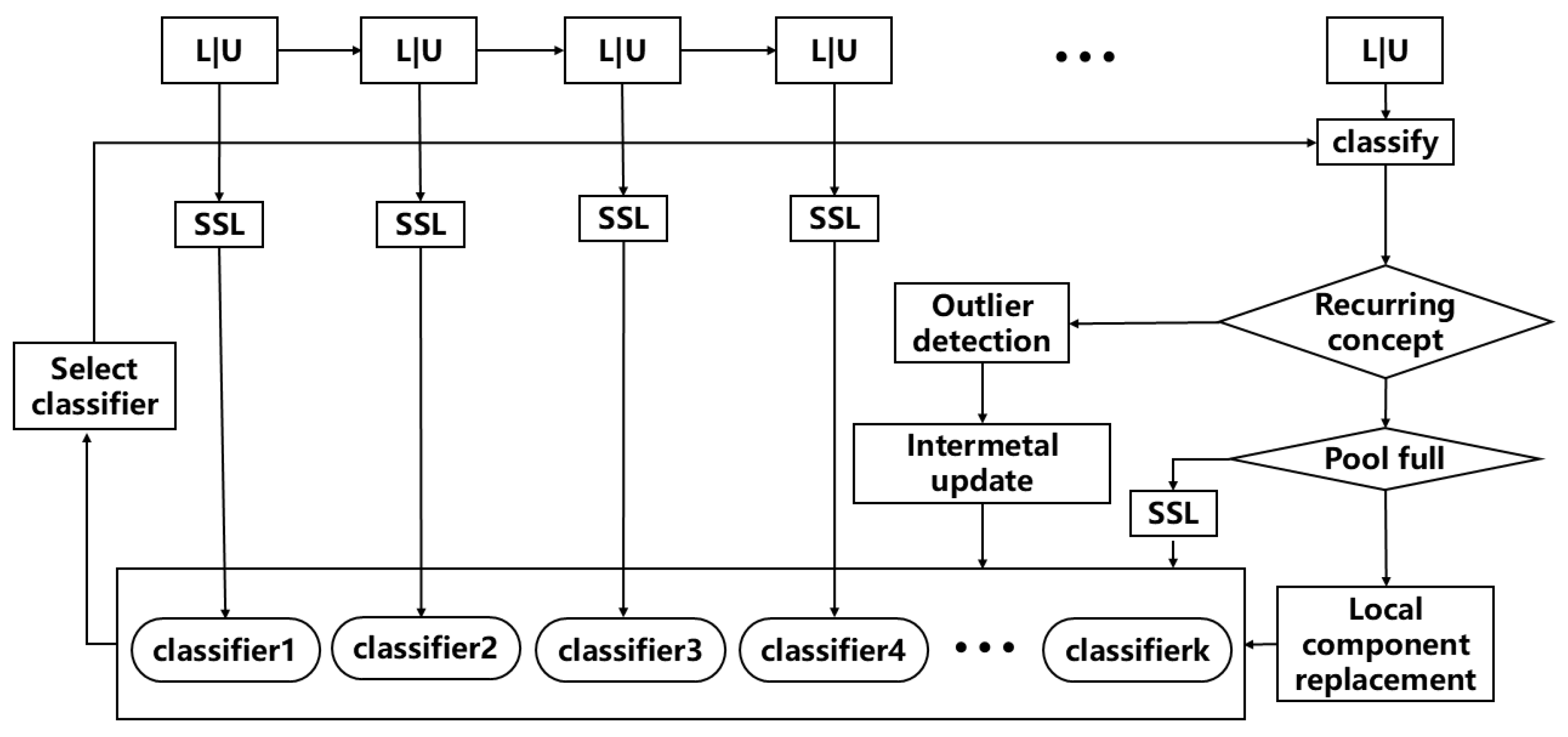
The flowchart of the SSCME algorithm is shown in Figure 1. When data streams arrive, the data are transmitted in the form of data blocks. Initially, a semi-supervised clustering algorithm is used to train the samples in the first data block (Block $D_0$), generating a classifier and placing it into the classifier pool with an initial weight of 1. As subsequent data blocks arrive, we first select the classifier with the highest weight in the pool to predict the sample’s classification. Based on the prediction result, the weight of the classifier is adjusted: if the prediction is correct, the weight remains unchanged, but if the prediction is incorrect, the weight is reduced. After classifying all the samples in the current data block, concept drift detection is performed to determine whether it represents a recurring concept, i.e., the reappearance of a previously encountered concept.

If the current data block represents a different concept than the one in the classifier pool, a new classifier is retrained using a semi-supervised classification algorithm and added to the classifier pool. If the classifier pool is full, we select the classifier that matches the classification criteria and meets the conditions for local component replacement. If the concept represented by the current data block is a recurring concept, we first perform anomaly detection on the samples in the data block and remove the abnormal data. The remaining samples are then updated incrementally using the appropriate classifier. Finally, the potential hazard trend is analyzed based on the prediction results. This approach allows for efficient handling of the data stream while maintaining an adaptive and accurate prediction system in dynamic environments.

3.2. Concept Drift Detection

Traditional concept drift detection methods are often based on accuracy, such as assuming that no concept drift has occurred if the classifiers in the classifier pool maintain high prediction accuracy on the current data block. However, this approach has several obvious issues, especially in dynamic environments like tunnel construction monitoring data. Specifically, accuracy-based detection methods mainly rely on the model’s prediction results to determine whether concept drift has occurred. The main problems with this method include lagging, inefficiency, and difficulty in handling high-dimensional and complex data.

Concept drift detection in the SSCME algorithm consists of two steps. In the first step, we determine whether the current data block is sufficiently similar to the historical classifiers to satisfy the conditions for calculating concept drift. If the conditions are met, we proceed to the second step. In this step, we train the current data block into a clustering-based classifier, where the k clusters are referred to as concept clusters ${\mu }_{new}$. We then select the classifiers from $C_1$ that meet the conditions, and their cluster centers are denoted as ${\mu }_{last}$. To measure the deviation between the clustering of ${\mu }_{new}$ and ${\mu }_{last}$, we define two variables: (i) r, which specifies the radius of the concept clusters ($r_{new}$ and $r_{last}$ represent the concept cluster radii in ${\mu }_{new}$ and ${\mu }_{last}$, respectively), and (ii) dist, which represents the distance between concept clusters, as shown in Equation (1):

$$\begin{array}{c}\hfill r=\sum _{i=1}^{m_p}\sqrt{\sum _{j=1}^{\left|A\right|}{\displaystyle \frac{{\left(m_{pj}-e_{ij}\right)}^2}{\left|m_p\right|}}}\end{array}$$

(1)

Here, $m_p$ refers to the current centroid of the $p^{th}$ cluster, $e_i$∈$m_p$, and $\left|A\right|$ represents the dimensionality of the attributes, with $|m_p|$ indicating the number of instances. The distance between two concept clusters, $m_l$ and $m_h$, refers to the Euclidean distance between their centroids with respect to the attribute set A, as shown in Figure 1.

$$\begin{array}{c}\hfill dist=\sqrt{\sum _{i=1}^{\left|A\right|}{(m_{l_i}-m_{h_i})}^2}\end{array}$$

(2)

In this case, we consider four different scenarios:

(1)

0 < dist ≤ |$r_{new}-r_{last}$|;

(2)

max($r_{new}$, $r_{last}$) < dist < $\alpha$ ($r_{new}+r_{last}$);

(3)

|$r_{new}-r_{last}$| < dist ≤ max($r_{new}$, $r_{last}$);

(4)

dist ≥ $r_{new}+r_{last}$.

When the first condition is met, we consider it as satisfying the condition of concept reproduction. The second case also falls under concept reproduction but may be influenced by noise. The third case is regarded as the result of gradual concept drift and incremental concept drift. The fourth case is considered as the result of abrupt concept drift. Next, based on the calculation results of concept deviation, we select a subset of clusters from the current data block to perform incremental updates to alleviate the problem of the EM algorithm’s inability to reach global optimality.

3.3. Outlier Detection

The Expectation-Maximization (EM) algorithm is a commonly used iterative optimization technique, primarily for handling problems involving hidden variables (or unlabeled data). It estimates model parameters by maximizing the likelihood function and consists of two steps: (1) E-step—Given the current parameter estimates, calculate the conditional expectation of the hidden variables. In other words, based on the current model parameters and observed data, infer the distribution of the unobserved latent variables. (2) M-step—Using the expected values obtained from the E-step, update the model parameters to maximize the log-likelihood function of the complete data. Specifically, based on the expectations computed in the E-step, the model parameters are re-estimated in a way that maximizes the likelihood of the data.

The EM algorithm alternates between the E-step and M-step until convergence or until a stopping criterion is met. It typically converges to a local optimum rather than a global optimum, especially when dealing with high-dimensional, complex data. The algorithm may become stuck in suboptimal solutions, which means its results can be influenced by the choice of initial parameters and may not guarantee the global optimum. To address this issue, before performing incremental updates, we need to eliminate anomalous data points to prevent them from negatively influencing the optimization process. Next, we describe how to detect anomalous points.

For sample $x_i$ in the data block, its $ϵ-$ neighborhood is defined as shown in Equation (3):

$$\begin{array}{c}\hfill N_{ϵ}\left(x_i\right)=\left\{x_j\in D|dist(x_i,x_j)\le ϵ|\right\}\end{array}$$

(3)

where D represents the data block and $dist(x_i,x_j)=\sqrt{{\sum }_{k=1}^n{(x_{i,k}-x_{j,k})}^2}$ represents the distance from point $x_a$ to point $x_b$. If $\left|N_{ϵ}\left(x_i\right)\right|<MinPts$, $x_a$ is marked as a noise point and removed from the data block, where $MinPts$ is the minimum point threshold we set. On this basis, we use kernel density estimation to determine $ϵ$, as shown in the following equation:

$$\begin{array}{c}\hfill f\left(x\right)={\displaystyle \frac{1}{nh}}\sum _{i=1}^{n}K\left({\displaystyle \frac{x-x_i}{h}}\right)\end{array}$$

(4)

where $f\left(x\right)$ is the density estimate at point X, n is the size of the data block, $K(•)$ is the kernel function, and h is the bandwidth. We calculate density estimates for each data point by selecting appropriate $K(•)$ and h, and select an appropriate density threshold $\rho$ based on the density estimation results, defining $ϵ$ such that the average density in the V domain of point x is equal to $\rho$, as shown in Equation (5):

$$\begin{array}{c}\hfill {\displaystyle \frac{1}{|N_{ϵ}\left(x\right)|}}\sum _{y\in N_{ϵ}\left(x\right)}f\left(y\right)=\rho \end{array}$$

(5)

In addition, $MinPts$ can be adjusted according to the distribution of the data. We use local density information, calculate the k-nearest distance $d_k\left(x_i\right)$ for each point $x_i$, and then define the following equation:

$$\begin{array}{c}\hfill {\rho }_i={\displaystyle \frac{k}{{\left(d_k\left(x_i\right)\right)}^{\alpha }}}\end{array}$$

(6)

where $\alpha$ is an adjustment parameter. We set $MinPts$ as a function related to the local density, i.e., $MinPts=\beta ·{\rho }_i$, where $\beta$ is a constant. The value of $MinPts$ is relatively large in higher-density regions and relatively small in lower-density regions.

3.4. Local Component Replacement

If the conditions for component replacement are met, we create a new classifier using the current data block. Then, we evaluate the classification ability of each component ${\varphi }_{ij}$ in the classifier pool $h_i$, using a vector, as shown in Formula (7), to assess the adaptability of each component in $h_i$ to the current data block:

$$\begin{array}{c}\hfill V_{ij}={\displaystyle \frac{NU{h}_{ij}}{N{U}_{ij}}}\end{array}$$

(7)

$N{U}_{ij}$ represents the number of samples in $D_t$ that the component ${\varphi }_{ij}$ of $h_i$ is involved in classifying, and $NU{h}_{ij}$ represents the number of samples in $D_t$ that it classifies correctly. Then, we replace the poorly performing components in $h_i$ with the closest components in $h_{new}$. The specific replacement method is shown in Equation (8):

$$\begin{array}{c}\hfill {\varphi }_{ij}=\left\{\begin{array}{c}{\varphi }_{new,k},\mathrm{if}N{U}_{ij}\ne 0\mathrm{and}{V}_{ij}<\tau \mathrm{and}arg\underset{1⩽m⩽\mu }{min}\left|{\mu }_{{\varphi }_{ij}}-{\mu }_{{\varphi }_{new,m}}\right|=k\\ {\varphi }_{ij},\mathrm{else}\end{array}\right.\end{array}$$

(8)

The symbol ${\mu }_{ij}$ represents the center of the $j^{th}$ component of the $i^{th}$ classifier, and $\tau$ is a pre-set constant that represents the minimum adaptability threshold. In the experiment, the value of $\tau$ is set to 0.5.

4. Experiments

4.1. Datasets

The dataset we created was sourced from multiple underwater tunnels. For each tunnel, we installed corresponding sensors and laser vibrometers to collect data, and the collected data were manually labeled. In addition, we selected several commonly used datasets in the field of machine learning, such as NEweather and Spam data, and generated some synthetic datasets using the MOA tool and version 3.7 Weka. Our dataset included both binary and multiclass samples, with varying sizes and block size settings for each dataset. The specific influence is shown in the following

Table 1. Properties of the datasets.

Dataset	Features	Classes	Instances	Chunk Size
Metro	4	2	1500	100
Spam data	5	2	9324	100
Hyperplane	10	2	200,000	1000
Sea	3	2	50,000	500
Gaussian	2	4	6000	300
NEweather	8	2	18,159	360
Spambase	57	2	4601	100
Cover type	54	7	581,012	1000
Electricity	8	2	45,312	1000
Kddcup99	41	23	494,020	1000
Poker hand	10	10	829,201	1000

. The other datasets we selected are described below.

Metro: This is a real dataset. The authors collected data by placing sensors in multiple tunnels to measure temperature, stress, pressure, etc. However, it is not yet possible to determine which concept drift this dataset conforms to. Further research is needed to improve the dataset.

Spam data: This dataset is derived from the Spam Assassin Collection. Each email is classified as either spam or ham, and the spam ratio is approximately 20%. The characteristics of spam messages in this dataset gradually change over time, i.e., gradual concept drift is simulated.

Hyperplane: This is an artificial dataset created using MOA. In dimensional space, the decision boundary of the hyperplane is determined by $f\left(x\right)=w_0-{\sum }_{i-1}^d{w}_i{x}_i=0$. Hyperplane is used to simulate incremental concept drift. The magnitude of change for each instance is set to 0.001.

Sea: This is an artificial dataset created using MOA, containing three features with values ranging between 0 and 10. Only two of the three attributes are relevant, while the other is redundant with a random value. The decision boundary of the concept is determined by $f\left(x\right)=a{x}_1+b{x}_2-\theta =0$. The threshold value is set to 8, 9, 7, and 9.5, corresponding to four concepts, denoted as f1, f2, f3, and f4, respectively. Concept drift occurs every 5000 samples, and the concept changes according to f1 -> f4 -> f3 -> f2 -> f3 -> f4 -> f3 -> f2 -> f1 -> f4.

NEweather: Initially introduced by Elwell et al., this dataset is collected from the Offutt Air Force Base in Bellevue, Nebraska, the target is to predict whether it will rain on a certain day. The imbalance toward no rain is 69%.

Cover type: This dataset contains information on forest cover types for 30 × 30 m cells in four wilderness areas located in the Roosevelt National Forest of northern Colorado. Only forests with minimal human-caused disturbances were used, so that the resulting forest cover types are primarily determined by ecological processes.

Electricity: This dataset contains information on price variation in the New South Wales (Australia) Electricity Market. A class label identifies the change in price relative to a moving average for the last 24 h. The concept changes result from changes in consumption habits, unexpected events, and seasonality.

Kddcup99: This dataset contains TCP connection records from two weeks of a network, which is widely used in the field of concept drift data streams. A subset of 10% of the data is used in our experiments.

Poker hand: This dataset contains instances representing all possible poker hands. Each card in a hand is described by two attributes: suit and rank. The class indicates the value of a hand. Here, we use the version described in [33], which sorts instances by rank and suit to simulate virtual concept drift while removing duplicate instances.

4.2. Experimental Setup

To evaluate the proposed algorithm, we compared it with two other algorithms: SPASC (the foundation of our work) and SSCLCR, an excellent clustering-based classifier. In SSCLCR, the detection of reoccurring concept drift employs a semi-supervised Bayesian approach. To ensure a fair comparison, the size of the classifier pool was set to 10, the proportion of labeled instances in the data blocks was set to 20%, the number of clusters K for all algorithms was set to 5, and the parameter $\tau$ was set to 0.5.

The proposed algorithm was implemented using the Weka package in a Java environment, with experiments conducted on a Windows Server 2012 R2 configured with 64 GB of RAM and a six-core CPU. During the experimental process, each data block was first used to test the current model, and then the model was updated before the next data block arrived. All experiments were repeated 10 times, with the positions of the labeled samples in the sample sequence changed each time to ensure the reliability of the results.

4.3. Proof of Innovation

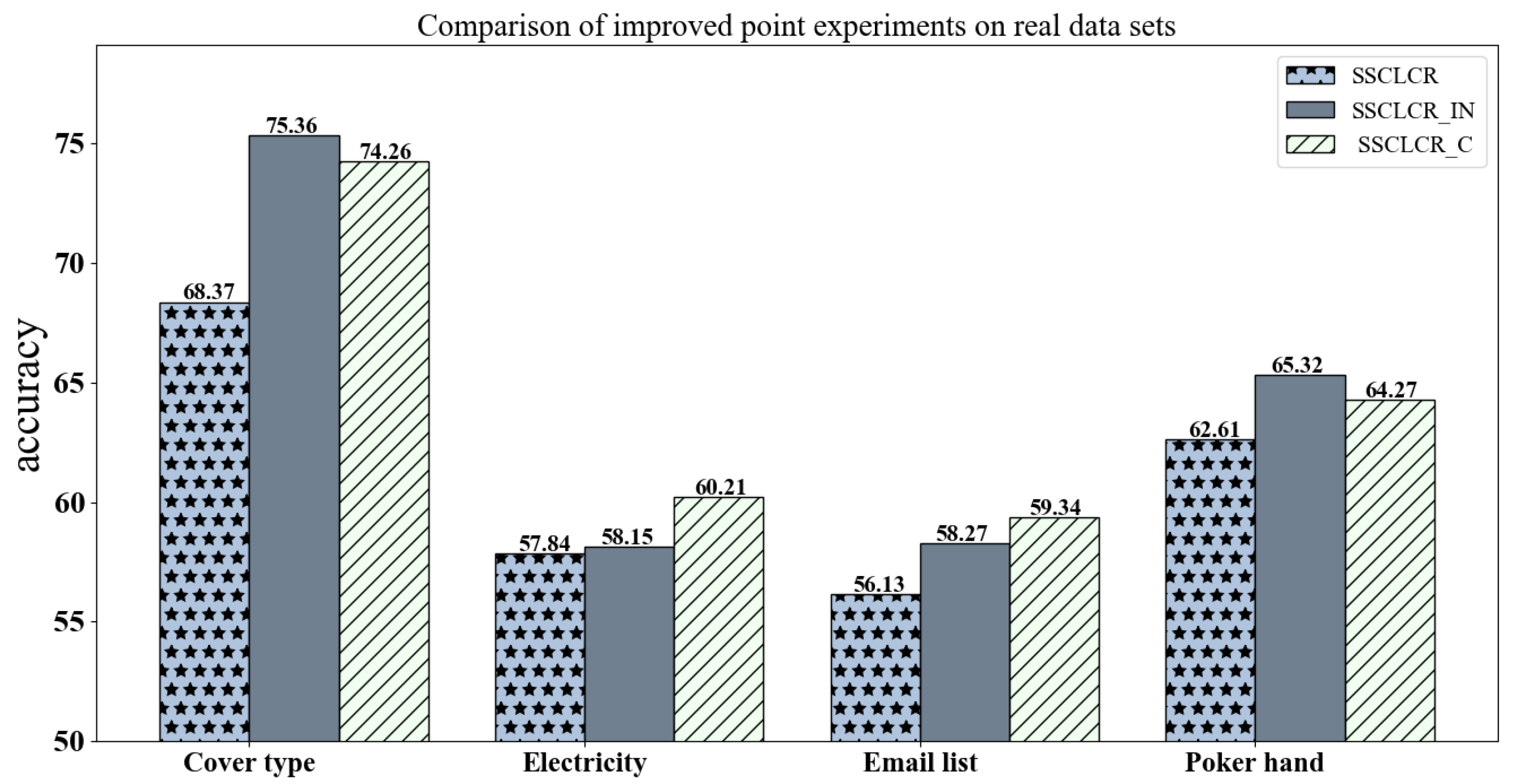
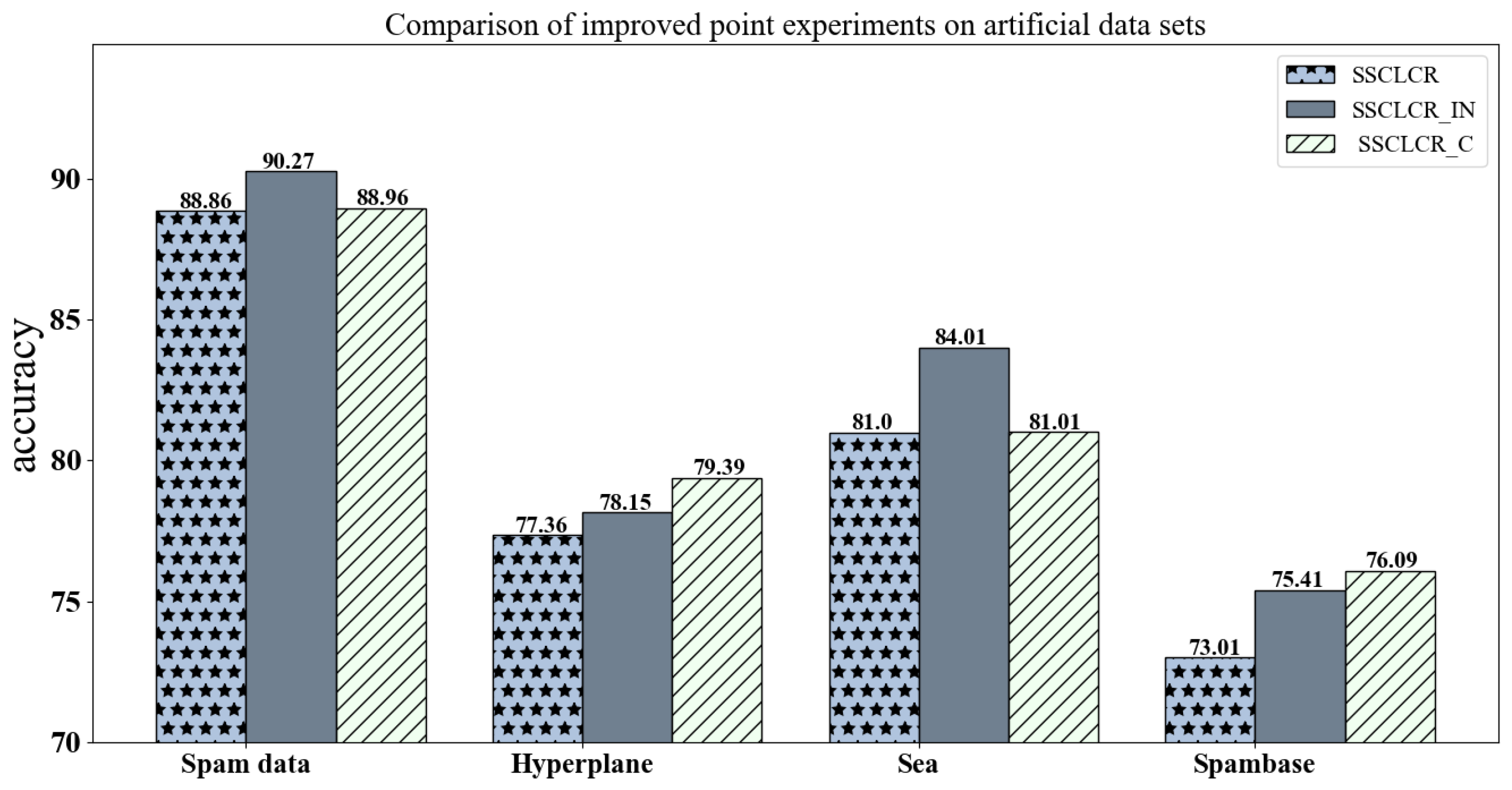
To validate the effectiveness of the proposed innovations, experiments were conducted on both real datasets, as shown in Figure 2, and artificial datasets, as shown in Figure 3, where SSCLCR_IN refers to the version with only improved incremental updates, and SSCLCR_C refers to the version with only updated concept drift detection.

The experimental results show that on the synthetic datasets, both improved algorithms performed better than the original algorithm, confirming the effectiveness of our innovations. At the same time, the results on the real-world datasets outperformed those on the synthetic datasets. This can be attributed to the fact that the synthetic datasets simulated sudden concept drift, where existing concept drift detection algorithms typically perform poorly due to their lack of robustness in handling abrupt changes. In contrast, the real-world “Cover type” dataset demonstrated a marked improvement, mainly because this dataset simulated gradual concept drift, and concept drift detection algorithms based on data distribution are more effective in handling gradual changes. These results highlight the advantages of our proposed methods, particularly in the context of more realistic, gradual concept drift scenarios commonly found in real-world applications.

4.4. Algorithm Comparison

Table 2. The average accuracy results (±standard deviation) over ten runs on each dataset.

Dataset	SSCME	SSCLCR	SPASC
Spam data	89.78 ± 0.57	88.86 ± 0.75	88.15 ± 1.08
Hyperplane	82.71 ± 0.55	77.36 ± 0.82	69.07 ± 0.97
Sea	81.97 ± 0.78	81.00 ± 0.56	78.86 ± 1.76
NEweather	68.32 ± 0.77	68.54 ± 0.86	68.70 ± 1.02
Spambase	98.01 ± 0.31	97.65 ± 0.33	97.52 ± 0.47
Gaussian	79.85 ± 1.54	73.01 ± 2.00	60.57 ± 0.90
Cover type	75.26 ± 1.30	68.37 ± 0.64	51.31 ± 5.52
Metro	61.06 ± 0.76	57.84 ± 0.63	56.61 ± 1.26
Electricity	59.20 ± 2.56	56.13 ± 3.01	56.27 ± 2.71
Kddcup99	97.83 ± 0.29	96.81 ± 0.37	96.82 ± 1.12
Poker hand	63.09 ± 0.18	62.61 ± 0.28	60.59 ± 1.36

shows the average accuracy results of the SSCME, SSCLCR, and SPASC algorithms on the 11 datasets. The average classification accuracy of SSCME was higher than that of SSCLCR and SPASC on ten datasets, especially on the Hyperplane, Cover type, Electricity, and Gaussian datasets, where the accuracy of the SSCME algorithm was significantly higher than that of SSCLCR and SPASC. Across all datasets, the accuracy of SPASC was generally lower than that of SSCLCR. This is because after the classifier pool is full, the SPASC algorithm always performs incremental updates regardless of whether the data corresponding to the current data block represent a concept drift, resulting in the updated classifiers not being able to adapt well to the new environment. The SSCLCR algorithm mitigates this problem by using component replacement. However, due to the classifier pool size being set to 10 and datasets such as NEweather, Electricity, and Kddcup99 containing fewer data, SSCLCR has to wait until the classifier pool is full before performing component replacement. This led to a small difference in the average accuracy between the two algorithms, and even on the NEweather dataset, the accuracy of SPASC was slightly lower than that of SSCLCR. On the Metro dataset, which is of particular focus, the proposed algorithm significantly outperformed the comparison algorithms, demonstrating that the chosen improvements are highly suitable for underground tunnel data. However, it is important to note that despite the overall lower performance of the algorithm on this dataset, we identified two primary reasons through analysis. First, noise issues during data collection were quite significant, which highlights a clear direction for future work. Specifically, it indicates the need for further data processing, including data augmentation and denoising steps, to improve the quality of the dataset. Second, our proposed algorithm’s model exhibited relatively weak noise resistance when handling high-dimensional data, another key factor influencing its performance. This limitation suggests the need for further refinement in the model’s ability to handle high-dimensional, noisy data, potentially through enhanced regularization techniques or more advanced noise-filtering strategies.

Table 3. Experimental results with different labeling ratios.

Dataset	Algorithm	0.1	0.2	0.3	0.4	0.5	0.6	0.7	0.8
Spam data	SSCME	92.87	93.74	93.84	94.18	94.26	94.79	95.01	95.51
	SSCLCR	87.20	88.86	89.48	89.90	89.88	90.30	91.07	90.36
	SPASC	85.71	88.15	88.98	89.37	89.98	90.46	91.00	90.96
Hyperplane	SSCME	79.30	80.71	81.72	81.89	81.76	81.91	82.32	83.50
	SSCLCR	73.60	77.36	78.83	79.62	79.44	80.45	80.20	80.26
	SPASC	50.24	50.49	50.31	51.25	54.91	61.92	71.40	81.03
Sea	SSCME	84.01	84.97	84.15	85.37	83.01	82.58	85.31	86.38
	SSCLCR	79.24	81.00	81.78	82.04	82.40	82.67	82.95	83.29
	SPASC	76.63	78.86	80.47	80.72	81.43	81.74	81.69	81.87
NEweather	SSCME	69.71	71.32	72.07	74.27	74.75	75.49	75.57	75.01
	SSCLCR	67.73	68.54	69.56	70.06	70.24	70.93	70.80	71.78
	SPASC	66.55	68.70	69.69	70.40	70.99	71.63	72.23	72.97
Spambase	SSCME	97.63	98.47	98.51	98.75	98.94	99.01	99.02	99.02
	SSCLCR	97.05	97.65	97.78	97.91	97.96	97.94	98.02	98.02
	SPASC	96.42	97.52	97.77	97.91	97.94	97.94	98.02	98.02
Gaussian	SSCME	73.76	75.85	76.07	76.59	76.94	77.67	78.06	78.09
	SSCLCR	71.53	73.01	74.76	75.60	74.92	75.35	76.42	76.15
	SPASC	59.21	60.57	61.07	61.60	62.33	62.34	62.87	62.52
Cover type	SSCME	77.36	78.26	78.89	79.21	80.31	80.45	82.98	84.07
	SSCLCR	67.74	68.37	68.73	69.29	69.93	69.89	69.91	69.71
	SPASC	53.37	51.31	55.62	54.18	57.76	57.96	58.78	57.84
Electricity	SSCME	61.37	62.20	64.07	64.41	65.39	65.87	65.96	66.42
	SSCLCR	53.69	56.13	59.62	62.32	64.81	66.81	69.34	69.80
	SPASC	53.69	56.27	59.44	62.71	64.96	66.89	69.29	69.73
Metro	SSCME	56.56	57.82	57.37	58.25	58.89	59.08	60.91	62.31
	SSCLCR	57.24	57.84	58.05	58.20	58.43	58.63	58.61	58.48
	SPASC	56.84	56.61	56.53	56.56	57.19	57.33	57.41	57.18
Kddcup99	SSCME	97.69	97.83	98.07	98.21	98.20	98.75	98.64	98.45
	SSCLCR	97.29	96.81	96.71	97.03	97.22	97.06	97.13	97.09
	SPASC	95.78	96.81	96.76	97.07	97.03	97.08	97.16	97.27
Poker hand	SSCME	62.94	63.09	63.24	63.98	64.41	64.76	64.81	65.12
	SSCLCR	61.94	62.61	62.84	62.88	62.88	62.86	62.97	62.74
	SPASC	61.05	60.59	61.19	61.25	61.02	61.09	60.76	60.40

shows the results of the influence of different labeling ratios on the classification accuracy of each algorithm. We increased the proportion of labeled samples from 10% to 80% at intervals of 10%. In most cases, the performance of SSCME was better than that of SPASC and SSCLCR. SSCME was particularly effective when the labeling ratio was low, as can be seen from datasets such as Spambase. On certain datasets, such as NEweather, Spam data, and Hyperplane, regardless of how the labeling ratio changed, the proposed algorithm consistently outperformed the comparison algorithms. Additionally, the classification accuracy of all three algorithms improved as the proportion of labeled samples increased. This is because, with more labeled samples, the model’s learning and generalization capabilities are enhanced, leading to better predictive performance. For the Metro dataset, when the labeling ratio was increased to eight times its original size, the classification accuracy improved by approximately 10%. This demonstrates that from an economic and time-efficiency standpoint, using a semi-supervised learning approach is a reasonable and effective choice. It allows for substantial improvements in performance without the need for a fully labeled dataset, making it a cost-effective solution in scenarios where labeled data are scarce or expensive to obtain.

5. Conclusions

This paper proposes a semi-supervised data stream classification algorithm, SSCME, for underground disaster monitoring and early warning. The algorithm first trains a model using data, and as new data arrive, the model is continuously updated. The updated model then predicts future trends, and appropriate responses are implemented based on the prediction results. The algorithm has two main innovations: (1) using data distribution to detect concept drift, and (2) an improved outlier detection method based on DBSCAN. The experimental results validate the effectiveness of the proposed algorithm.

Currently, predicting tunnel disasters using semi-supervised machine learning methods for data streams faces numerous challenges. The geological conditions, environmental changes, and construction processes in tunnels cause the monitored data to be time-varying, noisy, and incomplete, which makes it difficult for models to adapt to new data in real time. Furthermore, tunnel disaster data are often incomplete and imbalanced, and labeling is costly. Traditional methods, however, rely heavily on large amounts of labeled data. With the development of deep learning and incremental learning technologies, future efforts will focus on solving concept drift and missing data issues through more efficient model updates and adaptive learning methods. By integrating real-time monitoring data with multi-source information, future prediction systems will not only improve accuracy but also enhance tunnel disaster prediction and early warnings, providing intelligent decision support for tunnel construction.