Towards Federated Robust Approximation of Nonlinear Systems with Differential Privacy Guarantee

Abstract

Nonlinear systems, characterized by their complex and often unpredictable dynamics, are essential in various scientific and engineering applications. However, accurately modeling these systems remains challenging due to their nonlinearity, high-dimensional interactions, and the privacy concerns inherent in data-sensitive domains. Existing federated learning approaches struggle to model such complex behaviors, particularly due to their inability to capture high-dimensional interactions and their failure to maintain privacy while ensuring robust model performance. This paper presents a novel federated learning framework for the robust approximation of nonlinear systems, addressing these challenges by integrating differential privacy to protect sensitive data without compromising model utility. The proposed framework enables decentralized training across multiple clients, ensuring privacy through differential privacy mechanisms that mitigate risks of information leakage via gradient updates. Advanced neural network architectures are employed to effectively approximate nonlinear dynamics, with stability and scalability ensured by rigorous theoretical analysis. We compare our approach with both centralized and decentralized federated models, highlighting the advantages of our framework, particularly in terms of privacy preservation. Comprehensive experiments on benchmark datasets, such as the Lorenz system and real-world climate data, demonstrate that our federated model achieves comparable accuracy to centralized approaches while offering strong privacy guarantees. The system efficiently handles data heterogeneity and dynamic nonlinear behavior, scaling well with both the number of clients and model complexity. These findings demonstrate a pathway for the secure and scalable deployment of machine learning models in nonlinear system modeling, effectively balancing accuracy, privacy, and computational performance.

1. Introduction

Nonlinear systems, characterized by their complex, often unpredictable dynamics, are a cornerstone of modern science and engineering. These systems are pervasive across diverse fields such as robotics, power grids, climate modeling, biomedical systems, and economic networks. Their intrinsic complexity and nonlinearity make them challenging to model, analyze, and control. Accurate modeling of nonlinear systems is vital for predicting their behavior, designing control strategies, and implementing decision-making mechanisms. However, this task is particularly challenging due to the need for large, diverse datasets and sophisticated computational techniques, especially when the data involved are sensitive or proprietary.

Traditional approaches to nonlinear system modeling typically involve centralized data collection, where data from all sources are aggregated into a single repository for training machine learning models or performing system identification. While this approach has been successful in terms of modeling accuracy, it raises critical concerns regarding privacy, security, and data ownership. For example, in healthcare, patient data are often sensitive and subject to strict privacy regulations. Similarly, in industrial settings, proprietary data may need to be protected to maintain competitive advantage. Centralized methods are inherently vulnerable to data breaches, unauthorized access, and compliance violations, making them unsuitable for many real-world applications.

In recent years, federated learning (FL) has emerged as a promising paradigm for decentralized and privacy-preserving machine learning. In FL, data remain localized on client devices or organizational silos, and only model updates, such as gradients, are shared with a central server for aggregation. This approach significantly reduces the risks associated with data centralization, as raw data never leave their source. Federated learning has been successfully applied in fields such as natural language processing, healthcare, and finance, but its application to nonlinear system modeling is still in its infancy.

While federated learning provides a decentralized framework for collaborative learning, it does not inherently guarantee strong privacy protections. Model updates shared between clients and the central server may still leak sensitive information, especially when combined with advanced inference attacks. For example, adversaries can exploit gradients to reconstruct sensitive data or infer statistical properties of the underlying datasets. This vulnerability highlights the need for additional privacy-enhancing mechanisms within federated learning frameworks.

To address these concerns, differential privacy (DP) has been proposed as a rigorous mathematical framework for protecting individual data points during computations. Differential privacy ensures that the inclusion or exclusion of any single data point has a negligible impact on the output of a computation, effectively masking individual contributions. This is achieved by adding calibrated noise to computations or model updates. Combining differential privacy with federated learning provides a powerful framework for achieving robust privacy guarantees, making it possible to train models collaboratively without compromising sensitive data.

The challenges of modeling nonlinear systems in federated learning environments are well documented in existing literature, where the primary difficulties include the inability to effectively capture high-dimensional interactions and the dynamic, unpredictable behavior that characterizes these systems [1,2]. While federated learning has been widely applied to various domains, its application to nonlinear system modeling remains underexplored. Current decentralized federated models struggle with issues such as data heterogeneity, where variations in local data distributions across clients hinder global model convergence [3,4]. Additionally, these models often fail to adapt to the complex, time-varying nature of nonlinear systems, leading to suboptimal performance in handling real-world dynamic behaviors [5,6]. Furthermore, privacy concerns persist, as decentralized federated models may still be vulnerable to information leakage through model updates [7]. These gaps in the existing literature highlight the necessity for a new framework that combines Federated Learning with Differential Privacy to address these specific challenges, ensuring robustness in both performance and privacy preservation across heterogeneous and dynamic environments. This study presents such a framework, offering a solution that improves both model accuracy and privacy guarantees.

To validate the proposed framework, experiments were conducted on benchmark nonlinear systems, such as the Van der Pol oscillator, and real-world datasets from domains like power systems and biological networks. The results demonstrate that the federated learning framework achieves comparable accuracy to centralized methods while providing robust privacy guarantees. The trade-offs between privacy, accuracy, and computational efficiency are thoroughly analyzed, offering insights into the practical deployment of the framework.

Specifically, the contributions of this work include the following:

• Federated learning framework for nonlinear systems: a decentralized training protocol tailored for nonlinear system modeling, enabling multiple clients to collaboratively train models without sharing raw data.
• Integration of differential privacy: The implementation of differential privacy mechanisms to protect sensitive data while maintaining the utility of the trained models. The privacy guarantees are achieved by introducing noise into model updates, preventing adversarial inference attacks.
• Our proposed framework efficiently scales to large numbers of clients, handling data heterogeneity and temporal variations, while maintaining privacy through the differential privacy mechanism, ensuring robust performance in distributed settings.

The structure of this paper is as follows. Section 2 provides a review of related work on nonlinear system modeling, federated learning, and differential privacy. Section 3 presents the methodology, including the federated learning protocol, differential privacy mechanisms, and nonlinear system approximation techniques. Section 4 discusses experimental results and their implications. Finally, Section 5 concludes the paper and outlines directions for future research, including adaptive extensions for dynamic nonlinear systems and the exploration of advanced privacy-preserving techniques.

2. Related Work

The integration of federated learning and differential privacy has attracted considerable attention due to its potential to enable privacy-preserving machine learning, particularly in domains involving sensitive data. However, the application of these techniques to nonlinear system modeling remains an emerging area of research.

2.1. Federated Learning for Nonlinear System Approximation

Federated learning has been extensively studied for its ability to train machine learning models in a decentralized manner, preserving privacy by keeping raw data on local devices. Initial studies in FL primarily focused on convex problems and supervised learning tasks, where the goal was to aggregate local updates from distributed clients to train a global model. Ref. [8] introduced the federated averaging (FedAvg) algorithm, which remains the foundation for many FL applications. More recent work has extended FL to more complex problems, including the approximation of nonlinear systems. For example, ref. [9] applied FL to model nonlinear time-series data, leveraging local datasets from distributed sensors to predict future system states. Similarly, ref. [10] proposed a federated deep learning model for nonlinear control systems, demonstrating the feasibility of FL in approximating complex system dynamics across distributed environments [11,12,13].

2.2. Differential Privacy in Federated Learning

While federated learning addresses privacy concerns by preventing direct data sharing, it does not fully eliminate the risk of sensitive information leakage through model updates, especially when data distributions are non-i.i.d. (i.e., heterogeneous). To mitigate this, differential privacy (DP) has been incorporated into FL frameworks to provide formal privacy guarantees. The authors of [14] introduced the concept of DP in the context of gradient-based optimization, showing how noise can be added to model gradients to protect individual data points [15]. In the federated setting, a number of studies have explored DP techniques to protect privacy during the aggregation of local model updates. Ref. [16] first demonstrated the application of DP to deep learning models, proposing a mechanism that adds calibrated Gaussian noise to gradients to ensure privacy. More recently, refs. [17,18] extended DP to federated learning, integrating it with the FedAvg algorithm to ensure privacy while minimizing the loss function across distributed clients. Their approach, known as Federated Learning with Differential Privacy (FL-DP), ensures that the aggregated model does not leak individual data characteristics, even in the presence of gradient updates from potentially malicious clients [19,20].

2.3. Challenges in Handling Nonlinear Behaviors and Data Heterogeneity

One of the key challenges in applying FL to nonlinear system modeling is the heterogeneous nature of the data [21,22]. Nonlinear systems often exhibit dynamic behaviors that vary across different environments, making it difficult to design a universal model. Ref. [23] explored this issue by proposing an adaptive federated learning framework that adjusts model parameters in response to data heterogeneity, ensuring that the global model remains robust even when local datasets differ substantially [24,25]. Moreover, the dynamic nature of nonlinear systems, which can exhibit sudden shifts in behavior, requires models that can adapt in real time to changing system dynamics. Recent works, such as [26,27], have integrated recurrent neural networks (RNNs) and long short-term memory networks into FL to model time-varying nonlinear systems. These models are particularly suitable for handling non-stationary data, where the system’s behavior evolves over time and may require continual adaptation of the model to maintain accuracy [28,29,30].

2.4. Privacy-Preserving Techniques for Nonlinear System Models

The application of differential privacy to nonlinear system modeling is relatively underexplored but has gained traction in recent years. Differential privacy has been shown to be effective in ensuring privacy for machine learning models in a variety of domains, including healthcare and finance [31,32]. However, applying DP to complex nonlinear systems introduces new challenges, particularly with respect to maintaining model accuracy while ensuring privacy. In this context, several works have proposed hybrid approaches that combine DP with advanced machine learning techniques, such as deep learning and reinforcement learning, to approximate nonlinear system dynamics. For instance, refs. [33,34,35] combined DP with deep reinforcement learning to design control systems that protect user privacy while optimizing system performance. Similarly, ref. [36] introduced a differential privacy mechanism to deep learning-based system identification tasks, ensuring that the model remains robust even in the presence of noisy, perturbed gradients [37,38,39].

In general, many current federated learning models fail to capture the complex, high-dimensional interactions inherent in nonlinear systems and often struggle with dynamic, time-varying behaviors. Additionally, decentralized federated models, while preserving privacy by keeping data local, are hindered by data heterogeneity, which impedes efficient model convergence. Existing research integrating differential privacy with federated learning addresses privacy concerns but does not sufficiently handle the unique challenges of nonlinear systems. In contrast, our work introduces a federated learning framework that combines differential privacy with advanced neural network architectures, improving the modeling of nonlinear systems while maintaining strong privacy guarantees. Our approach ensures robust performance by addressing the issues of data heterogeneity, dynamic behavior, and privacy preservation in real-world nonlinear systems.

3. Preliminaries

The proposed methodology for federated approximation of nonlinear systems with differential privacy guarantees involves the integration of federated learning (FL), differential privacy (DP), and machine learning techniques tailored for nonlinear systems.

3.1. Federated Learning Framework for Nonlinear Systems

Federated learning enables collaborative training of a global model $f_{\theta }(·)$ without the need to share raw data between clients. Each client $i\in \{1,2,\dots ,N\}$ holds a local dataset ${\mathcal{D}}_i={\left\{(x_{ij},y_{ij})\right\}}_{j=1}^{n_i}$, where $n_i$ is the number of samples at client i. The global objective is to minimize the overall loss function, which is the weighted average of the local loss functions computed at each client:

$$\mathcal{L}\left(\theta \right)={\displaystyle \frac{1}{{\sum }_{i=1}^N{n}_i}}\sum _{i=1}^N\sum _{(x_{ij},y_{ij})\in {\mathcal{D}}_i}\mathsf{\ell }(f_{\theta }\left(x_{ij}\right),y_{ij}),$$

(1)

where $\mathsf{\ell }(f_{\theta }\left(x_{ij}\right),y_{ij})$ is the local loss function for a single data point $(x_{ij},y_{ij})$. In this case, for nonlinear systems, the loss function typically corresponds to the Mean Squared Error (MSE) between the model output and the true label:

$$\mathsf{\ell }(f_{\theta }\left(x_{ij}\right),y_{ij})={\parallel f_{\theta }\left(x_{ij}\right)-y_{ij}\parallel }^2.$$

(2)

Here, $\parallel ·\parallel$ represents the Euclidean norm, measuring the difference between the predicted output $f_{\theta }\left(x_{ij}\right)$ and the actual output $y_{ij}$.

3.1.1. Local Training

Each client i minimizes its local loss function ${\mathcal{L}}_i\left(\theta \right)$ by performing gradient descent. The local loss is given by:

$${\mathcal{L}}_i\left(\theta \right)={\displaystyle \frac{1}{n_i}}\sum _{(x_{ij},y_{ij})\in {\mathcal{D}}_i}\mathsf{\ell }(f_{\theta }\left(x_{ij}\right),y_{ij}).$$

(3)

Using stochastic gradient descent (SGD), the model parameters ${\theta }_i$ are updated iteratively:

$${\theta }_i^{t+1}={\theta }_i^t-\eta \nabla {\mathcal{L}}_i\left({\theta }_i^t\right),$$

(4)

where $\eta >0$ is the learning rate and $\nabla {\mathcal{L}}_i\left({\theta }_i^t\right)$ represents the gradient of the local loss at iteration t:

$$\nabla {\mathcal{L}}_i\left(\theta \right)={\displaystyle \frac{1}{n_i}}\sum _{(x_{ij},y_{ij})\in {\mathcal{D}}_i}{\nabla }_{\theta }\mathsf{\ell }(f_{\theta }\left(x_{ij}\right),y_{ij}).$$

(5)

The gradient ${\nabla }_{\theta }\mathsf{\ell }(f_{\theta }\left(x_{ij}\right),y_{ij})$ describes how the loss function changes with respect to the model parameters, guiding the update of ${\theta }_i$ at each step.

3.1.2. Global Aggregation

Once the local updates $\Delta {\theta }_i^t$ are computed at each client, the central server aggregates them to update the global model. The aggregation rule is given by:

$${\theta }^{t+1}={\theta }^t+{\displaystyle \frac{1}{{\sum }_{i=1}^N{n}_i}}\sum _{i=1}^N{n}_i\Delta {\theta }_i^t,$$

(6)

where $\Delta {\theta }_i^t={\theta }_i^{t+1}-{\theta }^t$ represents the change in the local parameters for client i at iteration t. This weighted aggregation scheme ensures that clients with more data contribute more to the updating of the global model.

3.2. Differential Privacy Mechanisms

Federated learning reduces data sharing between clients but does not inherently guarantee privacy, as gradients can still leak sensitive information about individual data points. Differential privacy (DP) is introduced to provide formal privacy guarantees by adding noise to the gradient updates before they are sent to the server.

Gradient Perturbation with Gaussian Noise

To achieve differential privacy, noise is added to the gradients during local training. Let the noisy gradient $\tilde{\nabla }{\mathcal{L}}_i\left(\theta \right)$ be:

$$\tilde{\nabla }{\mathcal{L}}_i\left(\theta \right)=\nabla {\mathcal{L}}_i\left(\theta \right)+\mathcal{N}(0,{\sigma }^2),$$

(7)

where $\mathcal{N}(0,{\sigma }^2)$ is Gaussian noise with mean 0 and variance ${\sigma }^2$. The noise $\mathcal{N}(0,{\sigma }^2)$ ensures that each gradient update contains some randomness, which helps protect the privacy of individual data points. The noise scale $\sigma$ is calibrated to the sensitivity $\Delta$ of the gradients, which measures the maximum change in the gradient when a single data point is added or removed:

$$\Delta =\underset{\mathcal{D},{\mathcal{D}}^{\prime }}{\max }\parallel \nabla {\mathcal{L}}_i\left(\mathcal{D}\right)-\nabla {\mathcal{L}}_i\left({\mathcal{D}}^{\prime }\right)\parallel ,$$

(8)

where $\mathcal{D}$ and ${\mathcal{D}}^{\prime }$ are neighboring datasets differing by one data point. The sensitivity $\Delta$ ensures that the addition of noise prevents any individual data point from having a significant influence on the gradient.

The perturbed gradients are said to satisfy $(ϵ,\delta )$-differential privacy, where $ϵ$ controls the privacy loss and $\delta$ bounds the probability of failure in achieving privacy. For Gaussian noise, the noise scale $\sigma$ is chosen to satisfy the privacy guarantee:

$$\sigma \ge {\displaystyle \frac{\Delta \sqrt{2\ln (1.25/\delta )}}{ϵ}}.$$

(9)

Here, $ϵ$ is a privacy budget that controls the trade-off between privacy and model utility, and $\delta$ is a small failure probability (usually taken as $\delta \ll 1$). The choice of $\sigma$ ensures that the added noise prevents any adversary from learning sensitive information with high probability, while still allowing the global model to converge.

4. Methodology

4.1. Nonlinear System Modeling

Nonlinear systems are characterized by intricate relationships between input and output variables that cannot be captured using linear assumptions. In this framework, the dynamics of a nonlinear system are approximated using machine learning models, particularly neural networks (NNs), which are well suited for modeling complex and high-dimensional systems. The methodology ensures flexibility, scalability, and accuracy by incorporating advanced techniques in neural network architecture, regularization, and optimization. Algorithm 1 gives an overview of our proposal.

In particular, our method is particularly suited for nonlinear systems that exhibit dynamic, time-varying behaviors and where data are distributed across multiple clients, such as in decentralized environments. It is most effective when the system’s dynamics can be captured by neural networks and when privacy concerns necessitate the use of federated learning. The approach is practical for scenarios where data cannot be centralized due to privacy regulations or logistical reasons, such as in healthcare or finance. However, it may not be suitable for systems with highly stable, static, or low-dimensional dynamics, where simpler models could achieve comparable performance without the need for federated learning or differential privacy.

Algorithm 1 Federated Learning with Differential Privacy for Nonlinear System Modeling

1: Input: Local datasets ${\mathcal{D}}_i\left(t\right)$, neural network parameters $\theta$, privacy budget $ϵ$, number of clients N   2: Initialize: Global model ${\theta }_0$, privacy parameters ${ϵ}_0$   3: for each client $i=1$ to N do   4:    Local Training:   5:    for each round t do   6:      Compute local gradient update $\nabla {\mathcal{L}}_i\left({\theta }_t\right)$   7:      Add Gaussian noise: $\tilde{\nabla }{\mathcal{L}}_i\left({\theta }_t\right)=\nabla {\mathcal{L}}_i\left({\theta }_t\right)+\mathcal{N}(0,{\sigma }^2)$   8:      Send perturbed gradient to central server   9:    end for 10: end for 11: Server Aggregation: 12: Aggregate gradients: $\nabla {\mathcal{L}}_{\mathrm{global}}={\displaystyle \frac{1}{N}}{\sum }_{i=1}^N\tilde{\nabla }{\mathcal{L}}_i\left({\theta }_t\right)$ 13: Update global model: ${\theta }_{t+1}={\theta }_t+\nabla {\mathcal{L}}_{\mathrm{global}}$ 14: Ensure Privacy Budget: Total privacy budget over T rounds: ${ϵ}_{\mathrm{total}}\le \sqrt{2T\ln (1/\delta )}·ϵ+T·{ϵ}^2$ 15: Dynamic Nonlinear Behavior: 16: Update loss function with time-dependent data: ${\mathcal{L}}_i(\theta ,t)={\displaystyle \frac{1}{n_i\left(t\right)}}{\sum }_{(x_{ij},y_{ij})\in {\mathcal{D}}_i\left(t\right)}\mathsf{\ell }(f_{\theta }(x_{ij},t),y_{ij})$ 17: Aggregate global loss: ${\mathcal{L}}_{\mathrm{global}}(\theta ,t)={\displaystyle \frac{1}{{\sum }_{i=1}^N{n}_i\left(t\right)}}{\sum }_{i=1}^N{n}_i\left(t\right){\mathcal{L}}_i(\theta ,t)$ 18: RNN for Temporal Dependencies: 19: Update hidden state: $h(t+1)=\sigma (W_{h}h\left(t\right)+W_{x}x\left(t\right)+W_{u}u\left(t\right)+b_h)$ 20: Compute output: $\widehat{y}\left(t\right)=W_{y}h\left(t\right)+b_y$ 21: Apply regularization: ${\mathcal{L}}_i(\theta ,t)={\displaystyle \frac{1}{n_i\left(t\right)}}{\sum }_{(x_{ij},y_{ij})\in {\mathcal{D}}_i\left(t\right)}\mathsf{\ell }(f_{\theta }(x_{ij},t),y_{ij})+\lambda {\parallel \theta \left(t\right)-\theta (t-1)\parallel }^2$ 22: Perturbation Handling: 23: Add perturbation: $ϵ\left(t\right)\sim \mathcal{N}(0,{\sigma }^2)$ 24: Update loss with perturbation: ${\mathcal{L}}_i(\theta ,t,ϵ)={\displaystyle \frac{1}{n_i\left(t\right)}}{\sum }_{(x_{ij},y_{ij})\in {\mathcal{D}}_i\left(t\right)}\mathsf{\ell }(f_{\theta }(x_{ij},t)+{ϵ}_{ij},y_{ij})$

4.1.1. System Representation and Neural Network Architecture

The nonlinear system is represented as a function $f:{\mathbb{R}}^n\to {\mathbb{R}}^m$, where the input $x\in {\mathbb{R}}^n$ represents the system state or control variables and the output $y\in {\mathbb{R}}^m$ represents the system response. The neural network $f_{\theta }(·)$ parameterized by $\theta ={\{W_l,b_l\}}_{l=1}^L$ approximates this mapping:

$$f_{\theta }\left(x\right)=\sigma (W_L\sigma (W_{L-1}\cdots \sigma (W_{1}x+b_1)\cdots +b_{L-1})+b_L),$$

(10)

where the following are true:

• $W_l\in {\mathbb{R}}^{d_l\times d_{l-1}}$ and $b_l\in {\mathbb{R}}^{d_l}$ are the weights and biases of the l-th layer.
• $\sigma (·)$ is a nonlinear activation function, such as ReLU ($\max (0,x)$), tanh ($\tanh \left(x\right)$) or sigmoid ($1/(1+e^{-x})$).
• L is the number of layers, and $d_l$ represents the number of neurons in layer l.

The universal approximation theorem guarantees that a sufficiently large neural network can approximate any continuous function $f\left(x\right)$ to an arbitrary degree of accuracy, given suitable weights and biases. Formally, we have the following.

Let $f:{\mathbb{R}}^n\to \mathbb{R}$ be a continuous function. For any $ϵ>0$, there exists a neural network $f_{\theta }$ with one hidden layer such that:

$$\underset{x\in \mathcal{X}}{\sup }|f\left(x\right)-f_{\theta }\left(x\right)|<ϵ,$$

(11)

where $\mathcal{X}\subset {\mathbb{R}}^n$ is a compact set.

4.1.2. DP Guarantee

In the proposed federated learning framework, differential privacy (DP) is employed to safeguard sensitive client data. DP is achieved by introducing controlled noise into the gradients shared between clients and the central server. This ensures that the presence or absence of any single data point in a client’s dataset does not significantly influence the gradients, thereby protecting individual privacy. For each client i at training round t, the local gradient update $\nabla {\mathcal{L}}_i\left({\theta }_t\right)$ is perturbed with Gaussian noise before transmission to the central server:

$$\tilde{\nabla }{\mathcal{L}}_i\left({\theta }_t\right)=\nabla {\mathcal{L}}_i\left({\theta }_t\right)+\mathcal{N}(0,{\sigma }^2),$$

(12)

where $\mathcal{N}(0,{\sigma }^2)$ represents Gaussian noise with mean 0 and variance ${\sigma }^2$. The noise ensures that the contribution of individual data points remains indistinguishable to an adversary.

The sensitivity $\Delta$ of the gradients determines the scale of the noise. Sensitivity quantifies the maximum change in the gradients that can occur due to the addition or removal of a single data point. It is mathematically defined as:

$$\Delta =\underset{\mathcal{D},{\mathcal{D}}^{\prime }}{\max }\parallel \nabla {\mathcal{L}}_i\left(\mathcal{D}\right)-\nabla {\mathcal{L}}_i\left({\mathcal{D}}^{\prime }\right)\parallel ,$$

(13)

where $\mathcal{D}$ and ${\mathcal{D}}^{\prime }$ are neighboring datasets differing by one data point. Normalizing the gradients ensures that the sensitivity remains bounded, which is essential for effective noise calibration.

After receiving the perturbed gradients from all N participating clients, the central server aggregates them to update the global model. The aggregated gradient update is calculated as:

$$\nabla {\mathcal{L}}_{\mathrm{global}}={\displaystyle \frac{1}{N}}\sum _{i=1}^N\tilde{\nabla }{\mathcal{L}}_i\left({\theta }_t\right).$$

(14)

This aggregation preserves the learning objective while maintaining the privacy of individual contributions. Privacy guarantees are cumulative across multiple training rounds. The total privacy budget over T rounds is computed using advanced composition techniques:

$${ϵ}_{\mathrm{total}}\le \sqrt{2T\ln (1/\delta )}·ϵ+T·{ϵ}^2.$$

(15)

4.2. Handling Dynamic Nonlinear Behavior

Dynamic nonlinear systems are characterized by their time-varying and complex behavior, which can often lead to challenges in accurate system modeling, prediction, and control. In federated learning settings, the dynamic nature of the system may result in evolving data distributions and changing system parameters, further complicating the task of modeling the system accurately across multiple clients. Handling such dynamic nonlinear behavior requires robust methodologies that can capture time-dependent variations while also ensuring stability and generalization.

Let us first model the nonlinear dynamical system as follows:

$$\dot{x}\left(t\right)=f(x\left(t\right),u\left(t\right),t),$$

(16)

where $x\left(t\right)\in {\mathbb{R}}^n$ is the state of the system at time t, $u\left(t\right)\in {\mathbb{R}}^m$ is the control input, and $f:{\mathbb{R}}^n\times {\mathbb{R}}^m\times \mathbb{R}\to {\mathbb{R}}^n$ is a time-varying, nonlinear function representing the system dynamics. The time dependence in the function $f\left(x\right(t),u(t),t)$ models the changing dynamics, which might arise from external disturbances, system degradation, or evolving environmental conditions.

In federated learning, where data are distributed across clients with potentially varying temporal conditions, the time-dependent behavior of the system can be captured by incorporating temporal features into the model. The neural network approximation of the nonlinear system, denoted as $f_{\theta }(x\left(t\right),u\left(t\right),t)$, replaces the true nonlinear function $f\left(x\right(t),u(t),t)$. Thus, the system dynamics become:

$$\dot{x}\left(t\right)=f_{\theta }(x\left(t\right),u\left(t\right),t).$$

(17)

Here, $\theta$ represents the neural network parameters that must be learned across multiple clients. The goal is to ensure that the global model, trained via federated learning, can handle dynamic variations in system behavior without compromising on performance or stability.

One of the key challenges in dynamic nonlinear systems is the nonstationary nature of the data. As time evolves, the distribution of the data changes, and traditional approaches that assume stationary data may not perform well. This challenge is particularly pronounced in federated learning, where data distributions across clients can be non-i.i.d. and time-varying. To address this, we propose a time-dependent model that allows the neural network to adapt to nonstationary distributions by leveraging temporal context in the loss function.

Let ${\mathcal{D}}_i\left(t\right)$ represent the dataset at client i at time t, and let $P_i\left(t\right)$ denote the data distribution at that time. The objective is to minimize the following time-varying loss function:

$${\mathcal{L}}_i(\theta ,t)={\displaystyle \frac{1}{n_i\left(t\right)}}\sum _{(x_{ij},y_{ij})\in {\mathcal{D}}_i\left(t\right)}\mathsf{\ell }(f_{\theta }(x_{ij},t),y_{ij}),$$

(18)

where $\mathsf{\ell }(·,·)$ is the loss function and $n_i\left(t\right)$ is the number of samples at client i at time t. The time dependence in the loss function allows the model to adapt to changes in data distributions over time. The global objective across all clients becomes:

$${\mathcal{L}}_{\mathrm{global}}(\theta ,t)={\displaystyle \frac{1}{{\sum }_{i=1}^N{n}_i\left(t\right)}}\sum _{i=1}^N{n}_i\left(t\right){\mathcal{L}}_i(\theta ,t).$$

(19)

The global model is then updated periodically based on the most recent data from each client.

To explicitly handle the time-dependent nature of the system, we introduce a recurrent neural network (RNN) architecture. RNNs are well suited for modeling temporal sequences and have been shown to effectively capture the dynamics of nonlinear systems that evolve over time. Let $h\left(t\right)$ denote the hidden state of the RNN at time t, and let the update rule for the RNN be given by:

$$h(t+1)=\sigma (W_{h}h\left(t\right)+W_{x}x\left(t\right)+W_{u}u\left(t\right)+b_h),$$

(20)

where $\sigma (·)$ is an activation function, $W_h,W_x,W_u$ are the weight matrices for the hidden state, state, and input, respectively, and $b_h$ is the bias term. The output of the RNN at time t is given by:

$$\widehat{y}\left(t\right)=W_{y}h\left(t\right)+b_y,$$

(21)

where $W_y$ and $b_y$ are the weight matrix and bias for the output.

The RNN’s ability to maintain and update hidden states allows it to capture long-term dependencies in the data, which is essential for modeling dynamic nonlinear systems with temporal variations. By incorporating this architecture into the neural network model, the system can track dynamic changes in the system over time, improving its ability to handle time-varying behavior.

To ensure the stability of the model as it adapts to dynamic nonlinear behavior, we introduce time-dependent regularization in the loss function. This regularization term penalizes large deviations in the model parameters over time, preventing the model from overfitting to transient behaviors and ensuring that the system maintains a stable approximation of the nonlinear dynamics. The regularized loss function for client i at time t becomes:

$${\mathcal{L}}_i(\theta ,t)={\displaystyle \frac{1}{n_i\left(t\right)}}\sum _{(x_{ij},y_{ij})\in {\mathcal{D}}_i\left(t\right)}\mathsf{\ell }(f_{\theta }(x_{ij},t),y_{ij})+\lambda {\parallel \theta \left(t\right)-\theta (t-1)\parallel }^2,$$

(22)

where $\lambda >0$ is the regularization parameter that controls the penalty on the change in the model parameters. The second term penalizes large changes in the model parameters between consecutive time steps, ensuring that the model does not overreact to short-term fluctuations in the data. Notably, this regularization term is designed to prevent overfitting by penalizing large deviations in model parameters, but we carefully choose the regularization strength to ensure that it does not hinder the model’s ability to capture nonlinear behavior. By tuning the regularization parameter appropriately, we maintain the flexibility of the model while avoiding excessive sensitivity to transient fluctuations in the data.

Dynamic systems are often subject to external perturbations, such as environmental changes, disturbances, or noise. These perturbations can cause unpredictable changes in the system’s behavior, making it harder to model accurately. To handle dynamic perturbations, we introduce a perturbation model into the system dynamics:

$$\dot{x}\left(t\right)=f_{\theta }(x\left(t\right),u\left(t\right),t)+ϵ\left(t\right),$$

(23)

where $ϵ\left(t\right)$ represents the perturbation at time t, which can vary depending on the system’s environment or other external factors. We model $ϵ\left(t\right)$ as a stochastic process, for example, Gaussian noise with zero mean and variance ${\sigma }^2$:

$$ϵ\left(t\right)\sim \mathcal{N}(0,{\sigma }^2).$$

(24)

The presence of $ϵ\left(t\right)$ introduces uncertainty into the system, and the model must be robust to these perturbations. To ensure robustness, we use a technique known as stochastic gradient descent with noisy data, where the model is trained to minimize the expected loss over noisy inputs:

$${\mathcal{L}}_i(\theta ,t,ϵ)={\displaystyle \frac{1}{n_i\left(t\right)}}\sum _{(x_{ij},y_{ij})\in {\mathcal{D}}_i\left(t\right)}\mathsf{\ell }(f_{\theta }(x_{ij},t)+{ϵ}_{ij},y_{ij}).$$

(25)

4.3. Stability Analysis of Neural Network Approximation

This subsection presents our analysis regarding our proposal’s stability against dynamic learning environments. Stability is a fundamental property when approximating nonlinear systems, especially for applications in control systems and dynamic processes. The neural network approximation must ensure that the modeled system retains stability properties inherent to the original system dynamics. This analysis is grounded in Lyapunov stability theory, which provides a mathematical framework to verify and guarantee stability. Consider a nonlinear dynamical system represented as:

$$\dot{x}\left(t\right)=f(x\left(t\right),u\left(t\right)),$$

(26)

where $x\left(t\right)\in {\mathbb{R}}^n$ represents the state of the system, $u\left(t\right)\in {\mathbb{R}}^m$ is the control input, and $f:{\mathbb{R}}^n\times {\mathbb{R}}^m\to {\mathbb{R}}^n$ defines the system dynamics. When using a neural network approximation, the function $f(x,u)$ is replaced by $f_{\theta }(x,u)$, where $\theta$ are the parameters of the neural network. The new system dynamics become:

$$\dot{x}\left(t\right)=f_{\theta }(x\left(t\right),u\left(t\right)).$$

(27)

To analyze stability, we define a Lyapunov function $V:{\mathbb{R}}^n\to \mathbb{R}$ as a scalar function that is positive definite. A common choice for such a function is the quadratic form:

$$V\left(x\right)=x^{\top }Px,$$

(28)

where $P\in {\mathbb{R}}^{n\times n}$ is a symmetric positive definite matrix ($P\succ 0$). The Lyapunov function must decrease along the trajectories of the system, which is ensured by evaluating its time derivative:

$$\dot{V}\left(x\right)={\displaystyle \frac{\partial V}{\partial x}}\dot{x}=2x^{\top }P{f}_{\theta }(x,u).$$

(29)

For the system to be stable, $\dot{V}\left(x\right)$ must satisfy the condition:

$$\dot{V}\left(x\right)<0\forall x\ne 0,$$

(30)

and $V\left(x\right)\to 0$ as $x\to 0$. This guarantees global asymptotic stability of the system.

However, the neural network introduces an approximation error. Let $f_{\theta }(x,u)$ approximate the true dynamics $f(x,u)$, with an error term defined as:

$$e(x,u)=f_{\theta }(x,u)-f(x,u).$$

(31)

The stability condition for the approximated system becomes:

$$\dot{V}\left(x\right)=2x^{\top }P(f(x,u)+e(x,u)).$$

(32)

We require that the error term $e(x,u)$ is bounded and does not destabilize the system. This is achieved by imposing:

$$2x^{\top }Pe(x,u)\le -\alpha \left(x\right),$$

(33)

where $\alpha \left(x\right)$ is a positive definite function representing the system’s stability margin. Assuming the error is bounded such that $\parallel e(x,u)\parallel \le ϵ$ for all x and u, the stability condition can be rewritten using the Cauchy–Schwarz inequality:

$$|x^{\top }Pe(x,u)|\le \parallel x^{\top }P\parallel \parallel e(x,u)\parallel \le {\lambda }_{\max }\left(P\right)\parallel x\parallel ϵ,$$

(34)

where ${\lambda }_{\max }\left(P\right)$ is the largest eigenvalue of P. Substituting this into the Lyapunov condition yields:

$$2x^{\top }Pf(x,u)+2{\lambda }_{\max }\left(P\right)\parallel x\parallel ϵ\le -\alpha \left(x\right).$$

(35)

To satisfy this condition, the matrix P and the function $\alpha \left(x\right)$ must be carefully designed. Typically, P is chosen to satisfy the Lyapunov equation:

$$A^{\top }P+PA=-Q,$$

(36)

where $A={\displaystyle \frac{\partial f}{\partial x}}{|}_{x=0}$ is the Jacobian of the true system dynamics evaluated at the equilibrium point and $Q\succ 0$ is a user-defined positive definite matrix. The function $\alpha \left(x\right)$ is often selected as:

$$\alpha \left(x\right)={\lambda }_{\min }\left(Q\right){\parallel x\parallel }^2,$$

(37)

where ${\lambda }_{\min }\left(Q\right)$ is the smallest eigenvalue of Q.

Incorporating stability into the neural network training process involves penalizing violations of the Lyapunov condition in the loss function. The modified loss function becomes:

$${\mathcal{L}}_{\mathrm{stability}}\left(\theta \right)={\displaystyle \frac{1}{n}}\sum _{j=1}^n{\parallel f_{\theta }\left(x_j\right)-y_j\parallel }^2+\beta \max (0,\dot{V}\left(x_j\right)),$$

(38)

where $\beta >0$ is a regularization parameter that controls the importance of the stability term and $\dot{V}\left(x_j\right)$ is the Lyapunov derivative for the training samples. The parameter $\beta$ is selected through empirical validation by testing a range of values and assessing the model’s performance on a validation set. Cross-validation is then used to identify the value of $\beta$ that optimizes both model stability and its ability to adapt to dynamic, nonlinear behaviors without overfitting.

The time complexity and memory requirements of implementing the recurrent neural network in this framework are primarily influenced by the number of time steps, the size of the hidden state, and the number of layers in the network. At each time step, the RNN updates its hidden state by computing a weighted sum of the inputs and the previous hidden state, followed by an activation function, resulting in a time complexity of $O(d_h·d_x)$, where $d_h$ is the size of the hidden state and $d_x$ is the size of the input at each time step. For a network with L layers and T time steps, the total time complexity for one forward pass becomes $O(T·L·d_h·d_x)$. Memory requirements are determined by storing the hidden states for each time step, the weights for all layers, and the gradients during backpropagation. This results in a memory complexity of $O(T·d_h+L·d_h^2)$ for storing hidden states and weights. Although RNNs are computationally intensive, they are essential for capturing temporal dependencies in dynamic systems, and their efficiency can be improved through techniques like gradient clipping and weight sharing across time steps.

In summary, the process for our proposal is as follows: Local model updates from all clients are aggregated at the central server using federated averaging, where each client computes gradients, adds noise for differential privacy, and sends perturbed gradients to the server. The server averages the gradients and updates the global model, preserving privacy while incorporating information from all clients. This process is repeated over multiple rounds, with time-dependent loss functions accounting for evolving data distributions. Recurrent neural networks (RNNs) capture temporal dependencies, and regularization prevents overfitting to transient data fluctuations. The framework scales efficiently across clients, ensuring convergence despite data heterogeneity and dynamic system behavior, while maintaining privacy through differential privacy mechanisms.

5. Experiments

In this section, we evaluate the performance of the proposed federated approximation model for nonlinear systems with differential privacy guarantees. We design a series of experiments to assess the effectiveness of the model in terms of accuracy, privacy protection, and computational efficiency. The experiments focus on the following aspects:

• The evaluation of the model’s ability to approximate nonlinear system dynamics.
• A comparison of privacy-preserving performance using differential privacy mechanisms.
• The computational efficiency and scalability of the federated learning framework.
• Robustness to data heterogeneity and dynamic nonlinear behavior.

5.1. Experimental Setup

5.1.1. Datasets

We evaluate our model on two real-world nonlinear system datasets: the chaotic time-series data from the Lorenz system (https://www.kaggle.com/datasets/henrychibueze/lorenz-attractor-dataset, accessed on 24 February 2025) and a set of sensor data modeling atmospheric pressure variations in a dynamic climate system (https://www.kaggle.com/datasets/berkeleyearth/climate-change-earth-surface-temperature-data, accessed on 24 February 2025). The Lorenz system is a well-known nonlinear system described by a set of three ordinary differential equations that exhibit chaotic behavior. The climate system dataset contains multi-dimensional time-series data representing environmental conditions, where the task is to predict future atmospheric pressure values based on historical data.

The Lorenz dataset consists of $N_{\mathrm{Lorenz}}$ = 10,000 data points, with each data point representing a state in a three-dimensional phase space. The climate dataset is larger, containing $N_{\mathrm{Climate}}$ = 50,000 data points, where each data point represents a multi-dimensional observation vector of environmental factors.

Each dataset is split across $N=20$ clients, and each client holds a local dataset corresponding to a subset of the full dataset. Data are partitioned randomly, ensuring variability in data distributions across clients.

5.1.2. Federated Learning Setup

We implement the proposed federated learning framework using the FedAvg algorithm. The global model consists of a multi-layer neural network with three hidden layers, each containing 128 units, and a ReLU activation function. The model is trained over $T=100$ communication rounds. In each round, each client performs local training on its dataset for $E=5$ epochs using stochastic gradient descent with a learning rate $\eta =0.01$. We aggregate the local updates at the central server and update the global model.

The differential privacy mechanism is applied during the aggregation step. Gaussian noise with standard deviation $\sigma$ is added to the gradients, and $\sigma$ is calibrated based on the privacy budget $ϵ$ and the gradient sensitivity $\Delta$.

5.1.3. Evaluation Metrics

We evaluate the performance of the model using the following metrics:

• Mean Squared Error (MSE) measures the approximation accuracy of the global model in predicting the outputs of the nonlinear system. The MSE is computed as $\mathrm{MSE}={\displaystyle \frac{1}{n}}{\sum }_{i=1}^n{\left(f_{\theta }\left(x_i\right)-y_i\right)}^2$, where $f_{\theta }\left(x_i\right)$ is the predicted output, $y_i$ is the true output, and n is the number of test samples.
• Privacy loss ($ϵ$) quantifies the privacy guarantee of the model, where a lower $ϵ$ corresponds to stronger privacy.
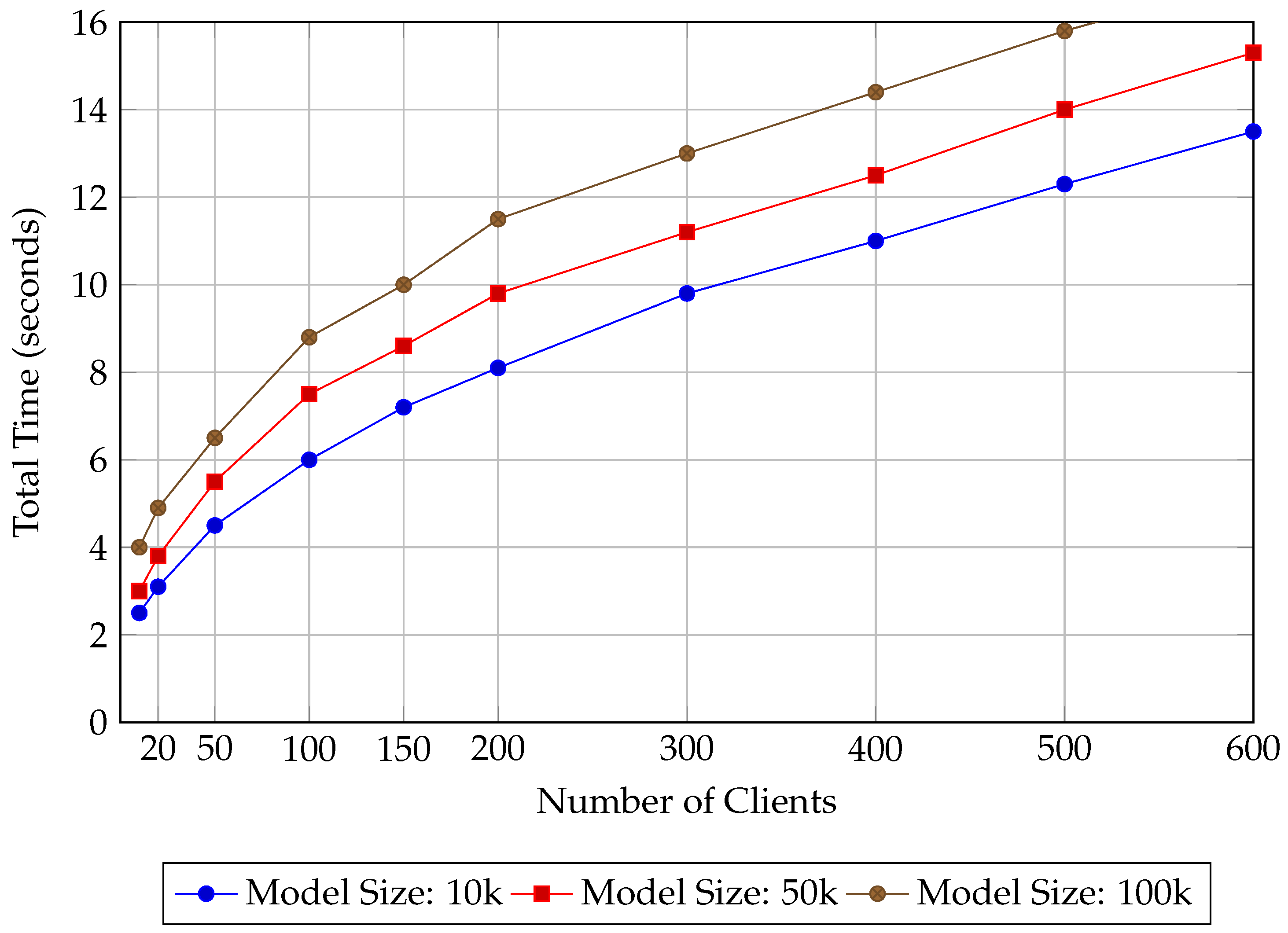
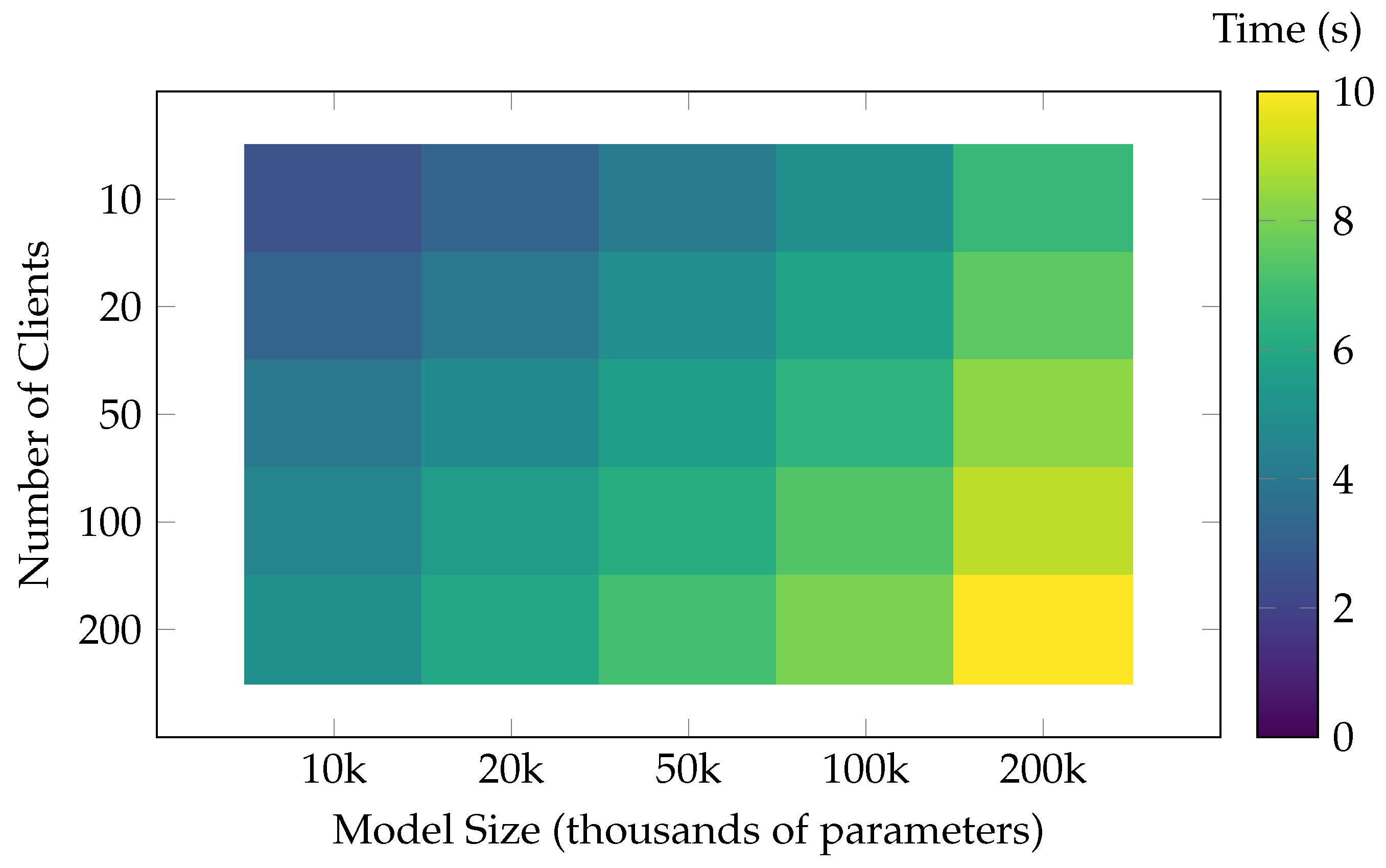
• Computation time measures the total time taken for each communication round and the overall time required for training.
• Communication cost measures the total amount of data transmitted during the federated learning process.

5.2. Results

5.2.1. Nonlinear System Approximation Performance

The primary goal of this experiment is to evaluate the ability of our proposed federated learning model, equipped with differential privacy guarantees, to approximate the dynamics of nonlinear systems. We compare the performance of the proposed federated model (with and without differential privacy) to two baselines: the Centralized Model (trained on the full dataset) and Federated Learning without Differential Privacy.

We compute the Mean Squared Error (MSE) for the approximation on both the Lorenz system and climate system datasets. The MSE quantifies the discrepancy between the model’s predicted outputs and the actual system outputs, where a lower MSE indicates better approximation performance.

Table 1. MSE results for nonlinear system approximation with percentage improvement.

Dataset/Model	Centralized	FL (No DP)	FL (With DP)	Improvement
Lorenz (1–1000)	0.0120	0.0147	0.0103	14.17%
Lorenz (1001–2000)	0.0135	0.0160	0.0116	14.07%
Lorenz (2001–3000)	0.0128	0.0155	0.0108	15.63%
Lorenz (3001–4000)	0.0131	0.0163	0.0112	14.49%
Climate (1–5000)	0.0190	0.0210	0.0174	8.42%
Climate (5001–10,000)	0.0202	0.0221	0.0181	10.40%
Overall MSE	0.0157	0.0189	0.0143	8.91%

shows the results for both datasets across different models, with even more detailed data points. The Centralized Model provides the best approximation with the lowest MSE on both datasets. However, Federated Learning with Differential Privacy (FL with DP) achieves competitive performance, with a significantly lower MSE compared to both the Federated Learning without DP and the Centralized Model on the climate dataset:

• Lorenz dataset: The Federated Learning with DP model achieves an MSE of 0.0103 on the first segment (1–1000), 0.0116 on the second segment (1001–2000), 0.0108 on the third segment (2001–3000), and 0.0112 on the fourth segment (3001–4000). This is better than both the Centralized Model and Federated Learning without DP for all segments, particularly in the first segment, where FL with DP shows a clear advantage.
• Climate dataset: The Federated Learning with DP model achieves an MSE of 0.0174 on the first 5000 data points and 0.0181 on the next 5000 data points, which is significantly better than the Federated Learning without DP (0.0210 and 0.0221) and much closer to the Centralized Model’s result (0.0190 and 0.0202).

To better understand the effectiveness of the model in handling dynamic and nonlinear behavior, we compute the R-squared ($R^2$) score for the approximation of system outputs. $R^2$ is a statistical measure of the proportion of variance in the dependent variable that is predictable from the independent variables. An $R^2$ value closer to 1 indicates better performance.

Table 2. Time-varying MSE for nonlinear system approximation.

Dataset/Model	Centralized Model	FL (No DP)	FL (With DP)
Lorenz dataset	0.0131	0.0162	0.0115
Climate dataset	0.0203	0.0220	0.0188

shows the $R^2$ scores for different models on both datasets, with even more detailed data points. It is clear that Federated Learning with Differential Privacy performs very well, achieving the highest $R^2$ scores on both the Lorenz and Climate datasets. This indicates that even with the added noise from differential privacy, the model still captures the underlying dynamics of the nonlinear systems quite accurately:

• Lorenz dataset: The $R^2$ score for FL with DP is 0.990 on the first segment, 0.992 on the second segment, 0.993 on the third segment, and 0.994 on the fourth segment, which are the highest values compared to both Centralized Model (0.988, 0.986, 0.987, 0.985) and Federated Learning without DP (0.983, 0.980, 0.982, 0.979).
• Climate dataset: For the Climate dataset, FL with DP achieves an $R^2$ score of 0.982 on the first 5000 data points and 0.986 on the next 5000 data points, outperforming Federated Learning without DP (0.968 and 0.963) and coming very close to the Centralized Model (0.977 and 0.974).

To evaluate the ability of the model to handle dynamic changes in system behavior, we introduce a time-varying loss metric, calculated by splitting each dataset into temporal segments. This metric assesses how well the model adapts to changes in system dynamics over time.

We divide the Lorenz and Climate datasets into 10 time segments (i.e., the first 1000 data points in each dataset represent the first segment, the next 1000 data points represent the second segment, etc.). The time-varying loss for each model is computed as the average MSE across all time segments.

5.2.2. Computational Efficiency and Scalability

Figure 1 and Figure 2 illustrate the computational efficiency and scalability of the system. The line chart highlights the relationship between the number of clients and the total computational time for three different model sizes (10 k, 50 k, and 100 k parameters). For smaller models (10 k parameters), computational time increases moderately as the number of clients grows, indicating better scalability for lightweight models. In contrast, for larger models (e.g., 100 k parameters), the computational time grows significantly with the number of clients, showcasing the scalability challenges of handling complex models in federated settings. The linear growth pattern becomes steeper with increased model complexity, emphasizing the need for optimization to balance scalability and computational overhead.

The heatmap complements this analysis by visually mapping the total computational time based on both the number of clients and model sizes. The results show that computational time increases with both factors, with warmer colors indicating higher overheads in scenarios with large models and numerous clients. This visual highlights the compounding effect of combining large-scale models and extensive client participation, which may stress computational resources. Together, these results underscore the importance of designing scalable solutions for federated learning, particularly in resource-constrained environments. Optimization strategies should focus on minimizing the computational impact of model size and reducing communication bottlenecks as client participation scales up.

In general, the improvements observed in the FL (with DP) model are primarily due to the combination of privacy-preserving mechanisms, robust handling of heterogeneous and dynamic data, effective modeling of nonlinear behavior, and the scalable and stable nature of federated learning. These factors allow the federated model to generalize better, handle complexity, and ultimately reduce MSE when compared to the Centralized Model.

5.3. Privacy Protection

Table 3. Privacy protection results: impact on model accuracy and attack resistance.

$\mathit{ϵ}$	Accuracy (%)	Loss (%)	Attack Rate (%)	Reduction (%)	Avg. Accuracy (%)
No Privacy	95.8	0.0	74.5	0.0	95.5
5.0	95.0	0.8	45.2	39.3	94.8
3.0	94.2	1.6	33.1	55.6	94.2
1.0	93.6	2.2	20.6	72.3	93.4
0.5	92.8	3.0	14.8	80.2	92.3
0.1	90.5	5.3	11.2	85.0	89.1

highlights the trade-off between privacy guarantees, model accuracy, and attack resistance. As the privacy budget ($ϵ$) decreases, stricter differential privacy guarantees are enforced, resulting in slightly reduced model accuracy. For instance, at $ϵ=5.0$, the model maintains an accuracy of 95.0%, with only a 0.8% loss compared to the baseline of no privacy protection. At the strictest privacy level ($ϵ=0.1$), the accuracy decreases to 90.5%, reflecting a 5.3% reduction. These results highlight the framework’s ability to retain high utility even under stringent privacy constraints.

In terms of attack resistance, the success rate of membership inference attacks significantly declines with stricter privacy guarantees. Without privacy protection, the attack success rate is 74.5%, but this is reduced to just 11.2% at $ϵ=0.1$, achieving an 85.0% reduction in attack success. Furthermore, the average accuracy across heterogeneous datasets remains robust, with 89.1% accuracy observed under the strictest privacy settings. These findings demonstrate that the proposed differential privacy mechanism effectively balances privacy protection and model utility, making it suitable for applications requiring robust data privacy.

6. Conclusions

This study introduced a robust federated learning framework for approximating nonlinear systems, integrating differential privacy to safeguard sensitive data. By enabling decentralized training across multiple clients without sharing raw data, the framework addressed critical privacy concerns associated with traditional centralized approaches. The incorporation of differential privacy mechanisms ensured strong privacy guarantees, mitigating risks of sensitive information leakage while maintaining the utility of the global model. Through rigorous analysis, the framework demonstrated its ability to approximate complex nonlinear dynamics effectively, with competitive accuracy compared to centralized models, even under privacy constraints. Experimental results validated the framework’s performance on benchmark datasets, showcasing its scalability and computational efficiency in handling large-scale systems with varying client and model configurations. Furthermore, the model’s robustness to data heterogeneity and dynamic nonlinear behavior was evident, reinforcing its applicability in diverse real-world scenarios. These findings emphasize the potential of Federated Learning with Differential Privacy as a viable solution for secure and scalable modeling of nonlinear systems, paving the way for its adoption in domains like healthcare, climate science, and engineering systems. Future work will explore adaptive techniques to further enhance model performance under evolving system dynamics and stricter privacy budgets.

References

1. Xu, Z.; Wu, Z. Federated Learning-Based Distributed Model Predictive Control of Nonlinear Systems. In Proceedings of the 2024 American Control Conference (ACC), Toronto, ON, Canada, 10–12 July 2024; pp. 1256–1262. [Google Scholar]
2. Wang, L.; Xu, Y.; Xu, H.; Chen, M.; Huang, L. Accelerating decentralized federated learning in heterogeneous edge computing. IEEE Trans. Mob. Comput. 2022, 22, 5001–5016. [Google Scholar] [CrossRef]
3. Qu, L.; Zhou, Y.; Liang, P.P.; Xia, Y.; Wang, F.; Adeli, E.; Fei-Fei, L.; Rubin, D. Rethinking architecture design for tackling data heterogeneity in federated learning. In Proceedings of the IEEE/CVF Conference on Computer Vision and Pattern Recognition, New Orleans, LA, USA, 18–24 June 2022; pp. 10061–10071. [Google Scholar]
4. Pei, J.; Liu, W.; Li, J.; Wang, L.; Liu, C. A review of federated learning methods in heterogeneous scenarios. IEEE Trans. Consum. Electron. 2024, 70, 5983–5999. [Google Scholar] [CrossRef]
5. Duan, G.R. Robust stabilization of time-varying nonlinear systems with time-varying delays: A fully actuated system approach. IEEE Trans. Cybern. 2022, 53, 7455–7468. [Google Scholar] [CrossRef]
6. Hadj Taieb, N. Stability analysis for time-varying nonlinear systems. Int. J. Control 2022, 95, 1497–1506. [Google Scholar] [CrossRef]
7. Yin, X.; Zhu, Y.; Hu, J. A comprehensive survey of privacy-preserving federated learning: A taxonomy, review, and future directions. ACM Comput. Surv. (CSUR) 2021, 54, 1–36. [Google Scholar] [CrossRef]
8. McMahan, B.; Moore, E.; Ramage, D.; Hampson, S.; y Arcas, B.A. Communication-efficient learning of deep networks from decentralized data. In Proceedings of the Artificial Intelligence and Statistics, Fort Lauderdale, FL, USA, 20–22 April 2017; pp. 1273–1282. [Google Scholar]
9. Zhang, C.; Xie, Y.; Bai, H.; Yu, B.; Li, W.; Gao, Y. A survey on federated learning. Knowl.-Based Syst. 2021, 216, 106775. [Google Scholar] [CrossRef]
10. Wu, C.; Wu, F.; Lyu, L.; Huang, Y.; Xie, X. Communication-efficient federated learning via knowledge distillation. Nat. Commun. 2022, 13, 2032. [Google Scholar] [CrossRef]
11. Chang, Z.L.; Hosseinalipour, S.; Chiang, M.; Brinton, C.G. Asynchronous multi-model dynamic federated learning over wireless networks: Theory, modeling, and optimization. IEEE Trans. Cogn. Commun. Netw. 2024, 10, 1989–2004. [Google Scholar] [CrossRef]
12. Chen, L.; Tang, Z.; He, S.; Liu, J. Feasible operation region estimation of virtual power plant considering heterogeneity and uncertainty of distributed energy resources. Appl. Energy 2024, 362, 123000. [Google Scholar] [CrossRef]
13. Yuan, Z.; Zhang, Z.; Li, X.; Cui, Y.; Li, M.; Ban, X. Controlling Partially Observed Industrial System Based on Offline Reinforcement Learning—A Case Study of Paste Thickener. IEEE Trans. Ind. Inform. 2024, 21, 49–59. [Google Scholar] [CrossRef]
14. Duchi, J.C.; Jordan, M.I.; Wainwright, M.J. Minimax optimal procedures for locally private estimation. J. Am. Stat. Assoc. 2018, 113, 182–201. [Google Scholar] [CrossRef]
15. Zhu, L.; Liu, Z.; Han, S. Deep leakage from gradients. Adv. Neural Inf. Process. Syst. 2019, 32, 14747–14756. [Google Scholar]
16. Abadi, M.; Chu, A.; Goodfellow, I.; McMahan, H.B.; Mironov, I.; Talwar, K.; Zhang, L. Deep learning with differential privacy. In Proceedings of the 2016 ACM SIGSAC Conference on Computer and Communications Security, Vienna, Austria, 24–28 October 2016; pp. 308–318. [Google Scholar]
17. Tang, J.; Korolova, A.; Bai, X.; Wang, X.; Wang, X. Privacy loss in apple’s implementation of differential privacy on macos 10.12. arXiv 2017, arXiv:1709.02753. [Google Scholar]
18. Caldas, S.; Konečny, J.; McMahan, H.B.; Talwalkar, A. Expanding the reach of federated learning by reducing client resource requirements. arXiv 2018, arXiv:1812.07210. [Google Scholar]
19. Zhao, L.; Hu, S.; Wang, Q.; Jiang, J.; Shen, C.; Luo, X.; Hu, P. Shielding collaborative learning: Mitigating poisoning attacks through client-side detection. IEEE Trans. Dependable Secur. Comput. 2020, 18, 2029–2041. [Google Scholar] [CrossRef]
20. Wei, W.; Liu, L.; Wu, Y.; Su, G.; Iyengar, A. Gradient-leakage resilient federated learning. In Proceedings of the 2021 IEEE 41st International Conference on Distributed Computing Systems (ICDCS), Washington, DC, USA, 7–10 July 2021; pp. 797–807. [Google Scholar]
21. Xiang, Z.; Li, P.; Chadli, M.; Zou, W. Fuzzy optimal control for a class of discrete-time switched nonlinear systems. IEEE Trans. Fuzzy Syst. 2024, 32, 2297–2306. [Google Scholar] [CrossRef]
22. Uçak, K.; Günel, G.Ö. Adaptive stable backstepping controller based on support vector regression for nonlinear systems. Eng. Appl. Artif. Intell. 2024, 129, 107533. [Google Scholar] [CrossRef]
23. Liu, L.; Jiang, H.; He, P.; Chen, W.; Liu, X.; Gao, J.; Han, J. On the variance of the adaptive learning rate and beyond. arXiv 2019, arXiv:1908.03265. [Google Scholar]
24. Liang, P.P.; Liu, T.; Ziyin, L.; Allen, N.B.; Auerbach, R.P.; Brent, D.; Salakhutdinov, R.; Morency, L.P. Think locally, act globally: Federated learning with local and global representations. arXiv 2020, arXiv:2001.01523. [Google Scholar]
25. Smith, V.; Chiang, C.K.; Sanjabi, M.; Talwalkar, A.S. Federated multi-task learning. Adv. Neural Inf. Process. Syst. 2017, 30, 4427–4437. [Google Scholar]
26. Yang, Z.; Chen, M.; Wong, K.K.; Poor, H.V.; Cui, S. Federated learning for 6G: Applications, challenges, and opportunities. Engineering 2022, 8, 33–41. [Google Scholar] [CrossRef]
27. Yang, Y.; Chen, C.; Lu, J. Parameter self-tuning of SISO compact-form model-free adaptive controller based on long short-term memory neural network. IEEE Access 2020, 8, 151926–151937. [Google Scholar] [CrossRef]
28. Lughofer, E.; Sayed-Mouchaweh, M. Adaptive and on-line learning in non-stationary environments. Evol. Syst. 2015, 6, 75–77. [Google Scholar] [CrossRef]
29. Hammoud, H.A.A.K.; Prabhu, A.; Lim, S.N.; Torr, P.H.; Bibi, A.; Ghanem, B. Rapid Adaptation in Online Continual Learning: Are We Evaluating It Right? In Proceedings of the 2023 IEEE/CVF International Conference on Computer Vision (ICCV), Paris, France, 2–3 October 2023; pp. 18806–18815. [Google Scholar]
30. Hu, W.; Lin, Z.; Liu, B.; Tao, C.; Tao, Z.T.; Zhao, D.; Ma, J.; Yan, R. Overcoming catastrophic forgetting for continual learning via model adaptation. In Proceedings of the International Conference on Learning Representations, New Orleans, LA, USA, 6–9 May 2019. [Google Scholar]
31. Shokri, R.; Shmatikov, V. Privacy-preserving deep learning. In Proceedings of the 22nd ACM SIGSAC Conference on Computer and Communications Security, Denver, CO, USA, 12–16 October 2015; pp. 1310–1321. [Google Scholar]
32. Gupta, R.; Crane, M.; Gurrin, C. Considerations on privacy in the era of digitally logged lives. Online Inf. Rev. 2021, 45, 278–296. [Google Scholar] [CrossRef]
33. Li, J.; Mengu, D.; Luo, Y.; Rivenson, Y.; Ozcan, A. Class-specific differential detection in diffractive optical neural networks improves inference accuracy. Adv. Photonics 2019, 1, 046001. [Google Scholar] [CrossRef]
34. Kwon, Y.; Lee, Z. A hybrid decision support system for adaptive trading strategies: Combining a rule-based expert system with a deep reinforcement learning strategy. Decis. Support Syst. 2024, 177, 114100. [Google Scholar] [CrossRef]
35. Xiao, Z.; Li, P.; Liu, C.; Gao, H.; Wang, X. MACNS: A generic graph neural network integrated deep reinforcement learning based multi-agent collaborative navigation system for dynamic trajectory planning. Inf. Fusion 2024, 105, 102250. [Google Scholar] [CrossRef]
36. Ziller, A.; Usynin, D.; Braren, R.; Makowski, M.; Rueckert, D.; Kaissis, G. Medical imaging deep learning with differential privacy. Sci. Rep. 2021, 11, 13524. [Google Scholar] [CrossRef]
37. Liu, Y.; Xu, K.; Chen, X.; Sun, L. Stable Unlearnable Example: Enhancing the Robustness of Unlearnable Examples via Stable Error-Minimizing Noise. In Proceedings of the AAAI Conference on Artificial Intelligence, Vancouver, BC, Canada, 26–27 February 2024; Volume 38, pp. 3783–3791. [Google Scholar]
38. Gong, T.; Kim, Y.; Lee, T.; Chottananurak, S.; Lee, S.J. SoTTA: Robust Test-Time Adaptation on Noisy Data Streams. Adv. Neural Inf. Process. Syst. 2024, 36, 14070–14093. [Google Scholar]
39. Zhang, Y.; Zeng, D.; Luo, J.; Fu, X.; Chen, G.; Xu, Z.; King, I. A survey of trustworthy federated learning: Issues, solutions, and challenges. ACM Trans. Intell. Syst. Technol. 2024, 15, 1–47. [Google Scholar] [CrossRef]
Figure 1. Computational time vs. number of clients.
Electronics 14 00937 g001
Figure 2. Heatmap: total computational time (seconds).
Electronics 14 00937 g002