Context Geometry Volume and Warping Refinement for Real-Time Stereo Matching

Abstract

In the past three years, the stereo matching method based on 3D CNNs has achieved surprising results and has received more and more attention. However, most stereo matching approaches aim to improve prediction accuracy by constructing and aggregating cost volumes through extensive 3D convolutions, which not only does not fully utilize the geometric information, but also overlooks the computational speed. Thus, achieving high-accuracy, high-efficiency stereo matching has become challenging. In this paper, we present a rapid and precise stereo matching network named CGW based on 3D CNNs, which simultaneously achieves real-time functioning, considerable accuracy, and a strong generalization capability. The network is divided into two parts. The first part constructs the geometric attention cube through a lightweight feature extraction network and a lightweight 3D regularization network. The second part filters the context features using the geometric attention cube to obtain the context geometric cube, and finally, the disparity is predicted and refined to obtain the final disparity. We adopted MobileNetV3 as an efficient backbone for feature extraction and designed 3D depthwise separable convolutions with residual structures to replace traditional 3D convolutions for constructing the cost volume and performing cost aggregation, aiming to reduce the model size and improve the computational speed. Additionally, we designed the context geometric attention (CGA) module and embedded it into the lightweight 3D regularization network, as well as designed the Warped Disparity Refinement (WDR) network to further improve the disparity prediction accuracy. CGA effectively guides cost aggregation by integrating rich contextual and geometric information, while also providing feedback for feature learning to guide more efficient context feature extraction. WDR constructs a warping cost volume using the obtained initial disparity, combined with image features, the initial disparity map, and reconstruction errors, to optimize the disparity. According to the initial disparity, it searches for the accurate disparity within a refined range. By narrowing the search range, WDR simplifies the task for the network to locate the correct disparity (residual), while simultaneously improving the computational efficiency. Experiments conducted on multiple benchmark datasets showed that, compared to other fast methods, CGW has advantages in both speed and accuracy and exhibits better generalization performance.

1. Introduction

Stereo matching is a key task in computer vision, aiming to estimate the depth information for each pixel in a binocular camera using a pair of stereo images. Specifically, stereo matching techniques calculate the disparity between corresponding pixel points in a stereo image pair. This process is based on the principles of the binocular vision of the human eye, simulating the way human eyes acquire depth information. Depth estimation plays a significant role in the real world and is a hot topic in current AI development, with applications such as intelligent assisted driving, cultural relic model reconstruction, and robot navigation. Despite numerous researchers having published their work, achieving efficient, fast, and accurate results with low computational complexity remains a significant difficulty and challenge, especially when dealing with image edge regions, repetitive structures, textureless areas, and transparent objects.

Traditional stereo vision matching involves four main steps: cost computation, cost aggregation, disparity estimation, and disparity refinement [1]. The cost computation is calculated by evaluating the similarity between corresponding pixels in a stereo image pair. Cost aggregation ensures that the matching of a pixel is constrained by the matching of its surrounding pixels, rather than considering the pixel in isolation, which considers the rationality of the matching cost of global information increases. Disparity estimation refines the cost volume and selects the disparity with the lowest cost for each pixel. Disparity optimization refines the initial disparity map to enhance result accuracy. With the advancement of CNNs, CNN-based stereo matching has demonstrated significant improvements. In general, the most efficient stereo matching models first utilize CNNs to extract deep features from stereo image pairs, then construct the cost volume by measuring the similarity of feature points between the stereo images in the pair, encoding local matching costs. However, these methods fail to incorporate non-local information, resulting in ambiguity in regions like reflective surfaces, large textureless areas, and occlusions [2]. To address this issue, researchers have proposed cost aggregation networks to aggregate contextual matching costs, combining local matching information with broader contextual information. GC-Net [3] builds a 4D cost volume based on the cost of feature points between stereo image pairs across various disparities and then infers the global geometry of the scene using a 3D encoder–decoder structure. PSMNet [4] and GwcNet [5] incorporate a new stacked 3D U-Net architecture to aggregate the cost volume. While these methods significantly enhance accuracy, they increase the network’s complexity and computational cost because of the extensive use of 3D convolutions. To mitigate memory and computational expenses, DeepPruner [6] introduces a PatchMatch module to ignore most irrelevant disparity candidates, effectively building a compact representation of the low-scale cost volume. GANet [7] includes two guidance aggregation layers to replace 3D convolutions [8], combines 3D and 2D CNNs for enhanced feature extraction, and integrates weighted median filtering to improve the boundary accuracy. AANet [9] introduced cost aggregation layers for within-scale and between-scale interactions. CoEx [10] enhances cost aggregation by utilizing the extracted image features, with weights derived from reference image features to adjust the channels of the cost volume. LNMVSNet [11] improves depth estimation, detail recovery, and feature clarity by strengthening the local feature focus and integrating multi-scale features. Fast-ACV [12] uses a lightweight correlation volume to create attention weights that refine the cascade volumes. However, these efficiency-focused models often lead to a notable decrease in accuracy, raising an important question: how can we effectively balance accuracy and computational speed?

In this paper, we present a disparity estimate model that is both accurate and fast, with strong generalization capabilities. For extracting valid features, we drew inspiration from the U-Net network structure. We began by utilizing a lightweight network to extract multi-scale features and then combined them to create a comprehensive feature map. Based on this feature map, we constructed a cost volume and a contextual feature cube. To obtain high-precision attention weights and disparity estimates, a common approach is to utilize 3D convolutions to concentrate the cost volume. Inspired by depth-separable convolutions in 2D convolutions, we designed the 3D convolutions as 3D depth-separable convolutions, which greatly lowered the model’s parameter count and computational load. Therefore, we designed a lightweight 3D regularization network to aggregate the cost volume. To leverage abundant geometric and contextual information, we propose an adaptive fusion of contextual information to guide cost aggregation, producing accurate cost volume attention weights to filter the contextual feature cube and generate the final contextual geometric cost cube. Additionally, we designed a disparity optimization module that constructs a warped cost volume, refining the disparity search range and enabling more accurate residuals in an unconstrained residual search space, while significantly reducing the network’s burden.

The key contributions of our study are as follows:

• We designed a lightweight multi-scale feature extraction structure and a 3D regularization network, transforming traditional 3D convolutions into 3D depthwise separable convolutions with a residual structure. This greatly lowered the model’s computational complexity while boosting its efficiency, leading to notable improvements in both accuracy and speed.
• We introduce contextual geometric attention (CGA), which adaptively fuses contextual information with geometric data to guide the determination of the cost volume in cost aggregation. This effectively improves the model’s accuracy and generalizability.
• We propose a Warped Cost Volume Disparity Refinement (WDR) module, incorporating left–right consistency checking to build the warped cost volume and inputting it, along with reconstruction errors and stereo image feature maps, into a residual network based on dilated convolutions to obtain refined disparity estimates.

2. Related Work

Stereo matching regresses the disparity from rectified left and right images. In recent years, deep stereo matching models based on end-to-end architectures designed with CNNs have flourished. Numerous researchers, through extensive experiments, have shown that cost volume building and aggregation, as well as disparity optimization, are key factors affecting the performance of disparity estimate models.

Cost volume construction and aggregation. Cost volume construction and aggregation primarily rely on convolutional neural networks to extract features from stereo image pairs and perform feature matching. DispNet [13] applies 2D convolutions for cost aggregation to fuse contextual information and directly regress disparity maps. Although using 2D convolutions significantly reduces the memory storage and computational complexity, it leads to the loss of substantial content information during the cost aggregation process, resulting in poor performance and unsatisfactory accuracy. IINet [14] introduces confidence-driven filtering and a rapid multi-scale sparse volume, using a more compact 2D implicit network. However, compared to 3D networks, it still results in the loss of information between stereo image pairs. GWCNet [5] proposes a group-wise correlation cost construction method, which groups the channels of the feature maps to build multiple disparity candidates, effectively addressing the redundancy issue of single-channel cost volume feature matching. Additionally, to better utilize the features extracted, it constructs two different cost volumes for concatenation. However, directly concatenating different cost volumes without considering their inherent relationships can make the concatenation process cumbersome. ACVNet [15], based on GWCNet [5], adds an attention mechanism. This mechanism generates geometry attention weights from group-wise correlation signals to filter out redundant information and improve the representation of relevant matching details in the cascaded volumes. Reliable attention weights are derived using the introduced multi-scale adaptive patch-matching technique. The aforementioned methods for cost volume construction and aggregation focus on utilizing contextual features to build the cost volume and apply 3D convolutions for aggregation. While they achieve good precision, the memory consumption and computational complexity also increase accordingly.

Meanwhile, some studies [12,14,16,17,18,19] focus on maximizing the real-time performance of the models while maintaining good precision. To achieve this, sparse or low-resolution cost volumes are typically constructed to decrease the number of parameters and the computation of the cost volume and subsequent cost aggregation. In [20], an initial matching cost volume was constructed by extracting stereo image pair features using 2D convolutions. After cutting the channel dimensions down with 1 × 1 convolutions, the cost volume was passed through a U-Net to predict the disparity. However, the use of 2D convolutions results in a severe loss of matching information, leading to a significant drop in accuracy. StereoNet [21] proposes an edge-preserving refinement network, which can be broken down into two phases. In the first phase, standard “linear” disparity prediction is performed, involving feature extraction to create multi-scale stereo image pair features and building a low-resolution cost volume to produce a coarse initial disparity. In the second phase, StereoNet concatenates the coarse disparity map and the left-view feature map generated in the first phase, using dilated convolution networks to learn and fill in edge details on the initial disparity map. However, relying solely on the left-view feature map to guide the restoration of details is inefficient and does not achieve satisfactory accuracy. BGNet [22] proposes a learning-based bilateral grid upsampling module that constructs a low-scale 4D cost volume and recovers the high-scale 4D cost volume. However, focusing only on the geometric information of the cost volume while ignoring the contextual information of image features leads to the insufficient accuracy of the details and a poor generalization ability. HITNet [18] processes the image hierarchically, refining a portion of the tiled regions at each iteration to reduce unnecessary computations and improve the speed. However, this approach often requires retraining for different datasets and has a poor generalization ability. PCVNet [23] parameterizes the cost volume by mapping each pixel’s disparity space to weights, means, and variances, mapping them to a multi-dimensional Gaussian distribution, and refining the cost volume through JS divergence. Fast-ACV [12] proposes the construction of multi-scale correlation volumes to generate the initial disparity and corresponding attention weights with a high likelihood, followed by the construction of sparse attention cascaded volumes. While these methods achieve better speed, their accuracy tends to decrease accordingly.

Disparity optimization. Once the initial disparity is obtained, many researchers [6,24,25,26,27] begin to optimize the initial disparity to obtain more accurate disparity maps; ref. [24] proposes a two-stage framework, where the first stage uses the DispNet [13] method to obtain the coarse disparity map and determine the approximate disparity region. The second stage searches for the precise disparity around the initial disparity using a residual network.The MCVMFC [26] method calculates reconstruction errors in the feature space, avoiding the limitations of directly computing errors in the pixel-level color space. Simultaneously, it enhances both performance and efficiency by enabling feature sharing between the disparity prediction and refinement networks. PCWNet [28] uses the initial disparity to obtain the distorted right-view features and computes the distorted cost volume to refine the disparity. However, the above three methods mainly focus on the post-processing part, optimizing the coarse initial disparity map, and do not place much emphasis on the fast and accurate acquisition of the initial disparity map, which would help reduce the optimization time and computational cost. RAFTStereo [29] and IGEV [30] utilize GRUs to iteratively update the disparity map from all related cost pairs. Selective Stereo [31] employs a new iterative update operator, selecting recursive units to gradually update the disparity map. The iterative update method can improve the disparity prediction accuracy to some extent, but it requires brief retraining each time during testing, meaning it is not a one-shot process.

3. Proposed Method

In this section, we present a comprehensive overview of the entire model, with the comprehensive architecture diagram shown in Figure 1. We first introduce the overall CGW network structure and then focus on explaining key components such as the 3D depthwise separable convolution, the context geometric attention (CGA) module, and the Warped Disparity Refinement (WDR) module. Finally, we explain the loss function used to train our CGW.

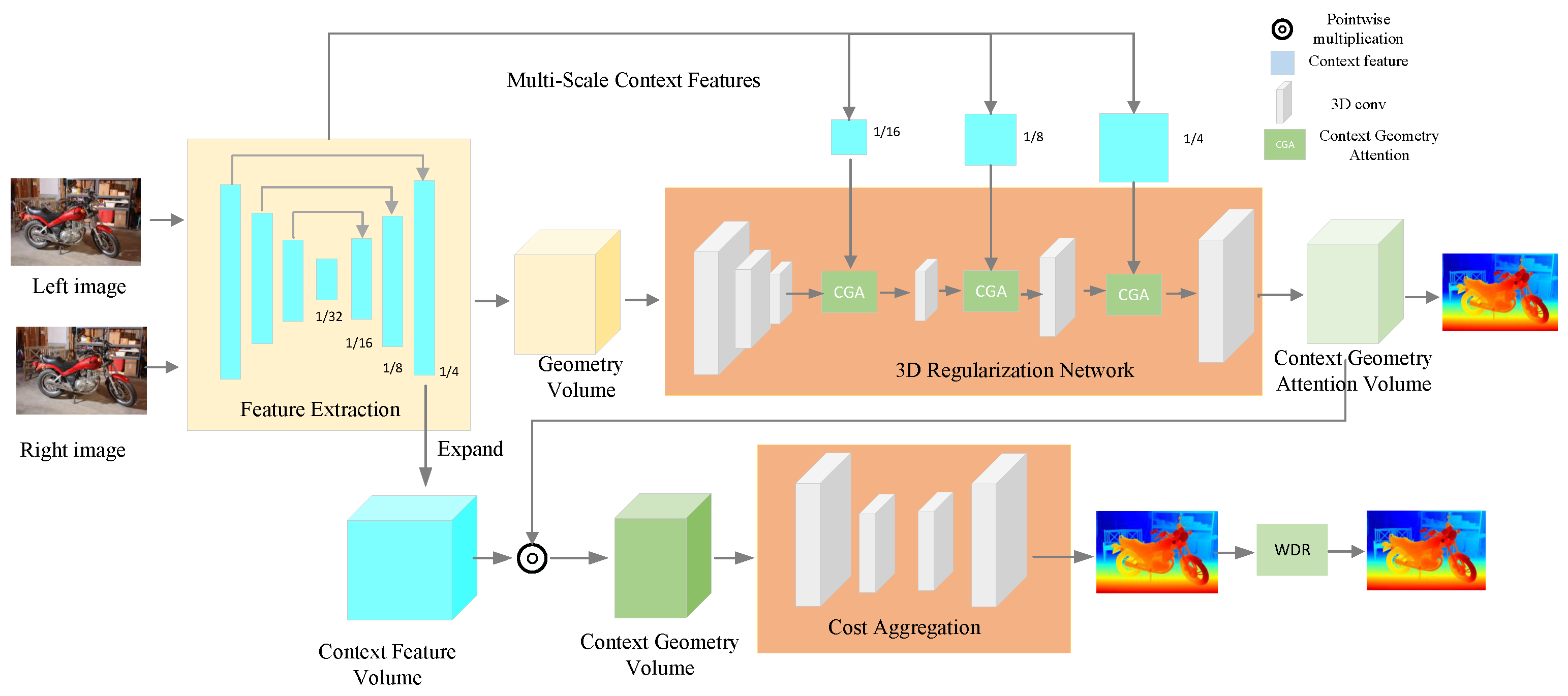
3.1. CGW Architecture

The CGW designed in this paper was divided into two parts. The first part included lightweight multi-scale fused feature extraction, initial cost volume construction, and the construction of a lightweight 3D regularization network. After training the first part, we obtained the geometry attention volume, which not only guided the training of the second part but also generated the attention-weighted disparity from the geometry attention volume to supervise the training of the entire network. The second part included context geometric attention cost volume construction, disparity prediction, and refinement, which combined contextual and geometric information to achieve more accurate results. Below, we will provide a detailed description of each part.

Lightweight Multi-Scale Feature Extraction. With the rapid development of convolutional upgrade networks, many high-quality feature extraction backbone networks have been proposed for extracting the deep features of images, such as ResNet [32] and GoogleNet [33], which are suitable for deep image feature extraction. Although these methods can obtain image features with rich information, they are often overly redundant and not ideal for real-time, efficient networks. Here, we propose a lightweight and useful multi-scale feature extraction network. Specifically, we utilized the pretrained MobileNetV3 [34] model as the backbone for multi-scale deep feature extraction in the lightweight network. By inputting left- and right-view images of the size H × W × 3, we utilized the ImageNet-pretrained MobileNetV3 network to extract four different-scale deep feature maps, i.e., downsampling the resolution by 1/4, 1/8, 1/16, and 1/32, with the channel number increasing correspondingly. At the same time, a standard convolution block was applied to extract the corresponding shallow features at each of the four scales. The deep and shallow features were then concatenated and fused to obtain four-scale stereo image pair feature maps, which contained rich local and global information. To more effectively fuse local and global contextual information, inspired by the U-Net network, we applied a 2D convolution layer to upsample the 1/32-scale feature map, generating the 1/16-scale feature map. The corresponding 1/16-scale feature map was then connected through a skip connection. Next, a channel attention module was used to adjust the significance of each channel, enhancing the context feature information scalability with a minimal computational cost and resource usage. This resulted in the fused 1/16-resolution feature map. We then continued to apply the same process to the 1/16-resolution feature map. Finally, we obtained a feature map at the 1/4 scale, which contained rich contextual information.

Initial Cost Volume Construction. We constructed an initial cost volume containing rich contextual feature information and geometric information using the 1/4-scale feature map. We extracted stereo image pair (left- and right-view image) features at the 1/4 scale, $f_l$ and $f_r\in R^{B\times C\times H/4\times W/4}$, then utilized the pre-set disparity threshold to build the initial cost volume $V_{int}$, which corresponded to the geometric volume in Figure 1.

$$\begin{array}{c}\hfill V_{\mathrm{int}}(x,y,d)={\displaystyle \frac{\langle f_l(x,y,d),f_r(x-d,y,d)\rangle }{\parallel f_l{(x,y,d)\parallel }_2·{\parallel f_r(x-d,y,d)\parallel }_2}}\end{array}$$

(1)

Here, x and y are the pixel horizontal and vertical coordinates on the feature map, and d is the disparity index. $f_l(x,y,d)$ and $f_r(x-d,y,d)$ represent the feature values of the left view at the pixel coordinates (x, y) and the corresponding feature values of the right view with a disparity offset of d. The cosine similarity of the disparity, d, corresponding to the feature points was used to compute the cost and then build the geometry volume (initial cost volume). The constructed geometry volume had only one feature channel. Therefore, we applied a series of operations such as 3D convolution, BatchNorm, and Leaky ReLU to increase the feature channels, resulting in a geometry volume at the 1/4 scale of $V_{int}\in R^{B\times C\times D/4\times H/4\times W/4}$.

Lightweight 3D Regularization Network. To combine feature information across both the spatial and disparity dimensions while incorporating rich contextual and geometric information, we designed a lightweight and useful 3D regularization network, R, to further process the initial cost volume $V_{int}$ at the 1/4 scale. The lightweight 3D network is composed of a 3D encoder–decoder module and a contextual geometric attention module. The 3D encoder–decoder module is a compact 3D U-Net made up of three 3D downsampling decoder blocks and three 3D upsampling encoder blocks. Each downsampling decoder block is composed of two 3 × 3 × 3 3D depthwise separable convolutions. The number of feature channels for the three downsampling decoder blocks are 32, 64, and 96, respectively. Each upsampling encoder block is composed of a 4 × 4 × 4 3D transposed convolution followed by two 3 × 3 × 3 3D depthwise separable convolutions. The 1/4-scale initial cost volume $V_{int}$ was fed into the three layers of the 3D decoder for downsampling to generate initial geometric volumes at the 1/8, 1/16, and 1/32 scales. These initial volumes were then input into the three layers of the 3D encoder for upsampling. Skip connections were used to fuse multi-scale geometric information, and at each upsampling step, the contextual geometric attention module was applied to integrate contextual features for cost aggregation. This generated the initial contextual geometric attention weight volume $A_{int}\in R^{B\times C\times D/4\times H/4\times W/4}$. Since the disparity values of the corresponding matching points exhibited a unimodal distribution, we reduced the size of the cost volume by compressing the disparity dimension of the attention weights. Only the top 12 most similar disparities were selected, significantly reducing the size of the contextual geometric attention weights and subsequent computations.Finally, the 3D regularization network output the context geometry attention volume $A_{cgv}\in R^{B\times C\times D^{\prime }\times H/4\times W/4}$, expressed as

$$\begin{array}{c}\hfill A_{\mathrm{cgv}}=R\left(V_{\mathrm{int}}\right)\end{array}$$

(2)

At the same time, we could also use the softmax function to apply a weighting to all disparity values for each pixel in the context geometric attention weight cube, in order to obtain the disparity value $d_{att}$ for that pixel in the corresponding stereo image pair.

Context Geometry Volume Construction. Grounded in the disparity index of the context geometry attention volume, we expanded and concatenated the feature maps from the left and right views at the 1/4 scale along the disparity dimension to form the context feature volume $V_c$:

$$\begin{array}{c}\hfill V_{\mathrm{c}}(x,y,d)=\mathrm{Expand}\{f_l(x,y,d),f_r(x-d,y,d)\}\end{array}$$

(3)

The dimensions of the context feature volume were B × 2C ×$D^{\prime }$× H/4 × W/4, containing rich contextual information. After obtaining the cost volume attention weights and the contextual feature volume, we utilized the context geometry attention volume to guide the determination of the context feature volume. This aided us in eliminating redundant information from the context feature volume and merging the geometric details from the attention weights to enhance the expressive capacity within the volume. The resulting context geometry volume $V_{cgv}$ was

$$\begin{array}{c}\hfill V_{\mathrm{cgv}}=A_{\mathrm{cgv}}\odot V_{\mathrm{c}}\end{array}$$

(4)

where ⊙ represents element-wise multiplication.

Disparity Prediction. The context geometry volume $V_{cgv}$ was first passed into the cost aggregation module, which is the 3D encoder–decoder module in the 3D regularization network, for cost aggregation. Then, for each pixel, the top 2 values were selected, and softmax was applied to these values to compute the weighted average. The resulting disparity map $d_0$ had a size of B × 1 × H/4 × W/4. Next, we used the “superpixel” weights [35] around each pixel to upsample the disparity map $d_0$ to the original scale, yielding $d_1\in R^{B\times 1\times H\times W}$.

3.2. 3D Depthwise Separable Convolution

The 3D regularization network was designed for cost aggregation, which is also the most time-consuming stage, with a large amount of 3D convolution. In cost aggregation, 3D convolution helps improve the accuracy, robustness, and generalization ability [36], but it typically consumes large amounts of memory and time during pretraining. Therefore, we considered modifying the structure of 3D convolution to reduce its computational burden, significantly improving its speed while maintaining its performance.

Firstly, we fed the stereo image pair into the multi-scale feature extraction module to obtain the corresponding features. These features contained rich contextual information. The resulting stereo image pair feature maps were used to build the cost volume. Finally, the 3D regularization network utilized the 3D encoder–decoder module (hourglass network) to aggregate the cost volume. The MobileNet [37] module was designed to replace 2D convolutions, with its core being depthwise separable convolutions. This approach splits 2D convolution into two efficient operations: depthwise convolution and pointwise convolution. It first increases the channel dimensions using a 1 × 1 convolution kernel, then performs convolution with a 3 × 3 kernel in the depthwise (DW) module, and finally reduces the channel dimension using a 1 × 1 convolution, forming a structure with small channels at both ends and a larger channel in the middle. This greatly lowers the model’s computational complexity and the number of parameters. Inspired by MobileNet, as shown in Figure 2, we extended 2D depthwise separable convolutions to 3D to handle the 4D cost volume. For this purpose, we applied depthwise and pointwise convolutions to the 3D convolution, expanding the dimensions of the input data from the original image feature (C,H,W) to the cost volume (C,D,H,W), where C is the number of feature channels, D is the disparity threshold for building the cost volume, and H and W represent the height and width of the input image features. Meanwhile, the convolution kernels were expanded to three dimensions, with the kernel size remaining consistent with that of the 2D version. For example, if the 2D convolution kernel size was k × k, the 3D convolution kernel size became k × k × k. The computational complexity was reduced from $O(C_{\mathrm{in}}·C_{\mathrm{out}}·D·H·W·k^3)$ to $O(C_{\mathrm{in}}·D·H·W·(k^3+C_{\mathrm{out}}))$.

3.3. Context Geometry Attention

To minimize the computational load, we built the cost volume using only low-scale features, which meant the context information contained in the cost volume was limited. To decode and obtain high-scale geometric information, we integrated contextual feature information with the cost volume to generate contextual geometric attention weights, which guided the cost aggregation process.

As shown in Figure 3, the left- and right-view images were passed through the network’s feature extraction module to extract rich multi-scale left- and right-view feature information, i.e., the contextual feature map $F_c\in R^{B\times C\times H\times W}$. Based on the similarity of the left- and right-view feature maps under different disparities, the corresponding cost volume was constructed, i.e., the geometric volume $F_G\in R^{B\times C\times H\times W}$, which contained rich geometric information. Here, B is the number of stereo image pairs that are processed in parallel by the input network at one time, H and W represent the height and width of the input stereo image features, D is the predefined disparity range for constructing the cost volume, and C is the number of feature channels. If only the geometric volume is used as the cost volume for cost aggregation, the result will not perform well in terms of the details. Therefore, we designed a context geometric attention (CGA) module to combine the contextual information of the contextual feature map with the geometric information of the geometric volume. We added a disparity dimension to the contextual feature map and expanded it along the disparity dimension to match our geometric information, represented as $F_{c^{\prime }}\in R^{B\times C\times D\times H\times W}$. For geometric information at different disparities, ideally, there is only one optimal disparity, i.e., the disparity dimension has a unimodal distribution [14]. However, the distribution of contextual feature information is based on pixel differences. To fuse these two, we considered both the feature and disparity dimensions to guide the cost aggregation, making the contextual feature information follow the distribution of the geometric information along the disparity dimension, and adaptively fused both pieces of information. We concatenated the contextual feature information and geometric information along the feature dimension and used 3D depthwise separable convolutions to preliminarily fuse both pieces of information to generate the Compact Concat Volume $V_{CG}$. Then, the sigmoid function was applied to activate the regions that should be emphasized or suppressed during the fusion process. The expression for the Compact Concat Volume $V_{CG}$ is as follows:

$$\begin{array}{c}\hfill V_{CG}=\sigma \left(\mathrm{conv}3\mathrm{d}\left(\mathrm{concat}\{F_c^{\prime },F_G\}\right)\right)\end{array}$$

(5)

In the formula, $\sigma$ represents the sigmoid activation function, conv3d denotes the 3D depthwise separable convolution operation from Section 3.1, and concat{,} signifies the concatenation of inputs. To better fuse the contextual information, we used the Compact Concat Volume $V_{CG}\in R^{B\times C\times H\times W}$ to guide the fusion of contextual feature information and geometric information to obtain the initial contextual geometric attention weights $A_{CF}\in R^{B\times C\times H\times W}$. Finally, the Compact Concat Volume $V_{CG}$, the initial contextual geometric attention weights $A_{CF}$, and the geometric volume $F_G$ were simply concatenated along the feature dimension to generate a cost volume containing rich contextual and geometric information, referred to as the fused volume G. The expressions for the initial contextual geometric attention weights $A_{CF}$ and the fused volume G are as follows:

$$\begin{array}{c}\hfill A_{CF}=V_{CG}\odot F_c^{\prime }\end{array}$$

(6)

$$\begin{array}{c}\hfill G=\mathrm{conv}3\mathrm{d}\left(\mathrm{concat}\{F_G,A_{CF},V_{CG}\}\right)\end{array}$$

(7)

where ⊙ denotes element-wise multiplication. Since we utilized contextual features at the 1/4, 1/8, and 1/16 scales and integrated them using 3D depthwise separable convolution, a large amount of contextual information was obtained while maintaining the same computational complexity. Meanwhile, the original complexity of $O(C_{\mathrm{in}}·C_{\mathrm{out}}·D·H·W·k^3)$ was reduced to $O(C_{\mathrm{in}}·D/n·H/n·W/n·(k^3+C_{\mathrm{out}}))$, where n represents the downscaling factor and k is the convolution kernel size. This significantly reduced the computation time.

3.4. Warping Disparity Refinement

Disparity refinement primarily involves the further optimization of the initial disparity obtained. As shown in Figure 4, we designed an efficient disparity refinement network that introduced multimodal inputs, including left features, the 4D warping cost volume, the initial disparity map, and the reconstruction error, allowing our network to more purposefully learn residual disparity values. First, we performed a warping operation (pixel coordinate shift), which shifted the coordinate axes of the right feature map according to the initial disparity. By adding the initial disparity information to the right feature map, the pixel positions in the right view could be adjusted according to the disparity of the left view, thus reducing the geometric differences between the left and right views and significantly decreasing the difficulty of subsequent optimization. Therefore, the application of the initial disparity map to the 1/4-scale right feature map to obtain the 1/4-scale warping right feature $f_{rw,4}$ is defined as

$$\begin{array}{c}\hfill f_{\mathrm{rw},4}=\mathrm{warping}(f_{r,4},d_0)\end{array}$$

(8)

where $f_{r,4}$ is the right feature map at the 1/4 scale, and $d_0$ is the initial disparity map. In theory, the right feature after disparity warping should perfectly match the left feature. However, due to the stereo model containing some errors, further optimization of the disparity was required. We calculated the cost between the left feature at each disparity level and the warped right feature to obtain the warping cost volume. Since the optimal disparity was simply around the initial disparity, the warping cost volume did not add much to the computation cost, while at the same time maximizing the positioning of the optimal disparity.

To construct the valid warping volume $V_w$, we utilized bilinear interpolation to obtain the original scale features from the left feature at the 1/4 scale and the warping right feature. The optimal disparity values are typically distributed within a certain range around the initial disparity d. Therefore, we defined a fine-grained residual search range, $\Delta d$, which narrowed the disparity search range from the initial range $(0,d_{max})$ to a more refined search range $(d-\Delta d,d+\Delta d)$. By reducing the size of the cost volume disparity dimension, the network’s task of finding the correct residual disparity was simplified. The 4D warping volume $V_w$ is expressed as follows:

$$\begin{array}{c}\hfill V_w(x,y,\Delta d)={\displaystyle \frac{\langle f_l(x,y,d),f_{rw}(x-d,y,d)\rangle }{\parallel f_l{(x,y,d)\parallel }_2·{\parallel f_{rw}(x-d,y,d)\parallel }_2}}\end{array}$$

(9)

where $f_l$ and $f_{rw}$ represent the left-view feature and the warping right-view feature, both linearly interpolated to the original scale, $\Delta d$ represents the fine-grained residual search range, and $\langle ,\rangle$ denotes the inner product.

Then, inspired by the classical left–right consistency check in traditional stereo matching disparity post-processing, we used the reconstruction error to direct the refinement module’s attention towards the regions of the initial disparity map that were incorrect. This allowed our refinement network to better identify disparities that needed further optimization, seeking precise disparities in error regions. The reconstruction error is expressed as follows:

$$\begin{array}{c}\hfill Error=\left|f_l(x,y,d)-f_{rw}(x-d,y,d)\right|\end{array}$$

(10)

Finally, we concatenated the left feature map, the 4D warping volume, the reconstruction error, and the initial disparity map as the multimodal input to the Warping Disparity Refinement network. Since the disparity dimension D of the warping cost volume was only 2 ∗ $\Delta d$, it was nearly negligible. As a result, the computational complexity of the 3D separable convolution was reduced to $O(C_{\mathrm{in}}·2\ast \Delta d·H·W·(k^3+C_{\mathrm{out}}))$. Additionally, dilated convolution was applied later to further enhance the computational efficiency. The input first passed through four convolution blocks, each consisting of a dilated convolution layer, batch normalization, and an activation function. These blocks progressively increased the dilation rate and enabled the network to capture features at multiple scales and broaden its field of view, while retaining crucial local details without adding extra parameters or computation. Next, the input passed through three residual blocks to support a deeper network structure without encountering gradient vanishing problems. Each residual block contained two dilated convolutions, followed by a convolution layer that generated the refined residual disparity. This was then added to the initial disparity to obtain the final disparity map.

3.5. Loss Function

The entire model was trained in a supervised end-to-end fashion. Compared to the $L_2$ loss, the $L_1$ loss is more robust to outliers, reducing the impact of large errors and, in some cases, promoting sparsity in the model. We therefore used the $L_1$ loss to measure the discrepancy between the predicted disparity and the truth disparity provided by the training dataset. The final loss function can be expressed as

$$\begin{array}{c}\hfill L={\lambda }_{\mathrm{att}}·{\mathrm{Smooth}}_{L_1}(d_{\mathrm{att}}-d_{\mathrm{gt}})+\lambda ·{\mathrm{Smooth}}_{L_1}(d-d_{\mathrm{gt}})\end{array}$$

(11)

where $d_{att}$ and $d_{gt}$ are the attention-weighted disparity obtained from the context geometry attention volume and the ground truth disparity. ${\lambda }_{att}$ and $\lambda$ are coefficients for the estimated attention-weighted disparity and the final estimated disparity, respectively. ${Smooth}_{L_1}$ represents the smooth $L_1$ loss, as follows:

$$\begin{array}{c}\hfill {\mathrm{Smooth}}_{L_1}\left(x\right)=\left\{\begin{array}{cc}0.5x^2,\hfill & \mathrm{if}\left|x\right|<1\hfill \\ \left|x\right|-0.5,\hfill & \mathrm{otherwise}\hfill \end{array}\right.\end{array}$$

(12)

4. Experiment

4.1. Datasets and Evaluation Metrics

Scene Flow [13] is a widely used benchmark for optical flow estimations and disparity estimations. For the disparity estimations part, this dataset provides data for three scenes, with the training dataset consisting of 35,454 synthetic binocular images and disparities, while the test dataset contains 4370 synthetic binocular images, both with a resolution of 960 × 540. In order to analyze the results, we used the End-Point Error (EPE) and Disparity Outliers (D1s) as our evaluation metrics. The EPE measures the End-Point Error between the estimated and the actual disparity for each pixel. The overall disparity estimation error is computed as the average EPE across all pixels. The N-px represents the percentage of pixels with a disparity error greater than a specific threshold, N, indicating that the disparity prediction for those pixels is incorrect. D1s are defined as the percentage of pixels where the disparity error exceeds the maximum of 3 px or 0.05$d^{*}$, where $d^{*}$ represents the true disparity. A D1 relaxes the 3 px error threshold by excluding pixels with relative absolute errors smaller than 5%.

KITTI [38,39] is a widely used public dataset that contains real-world driving scenes. The KITTI dataset includes KITTI 2012 [38] and KITTI 2015 [39]. The stereo image pairs in these two datasets were captured by two high-resolution cameras mounted on a car, with an image resolution typically of 1242 × 375 pixels. The KITTI 2012 dataset consists of 194 real-world driving image pairs for training and 195 pairs for testing, whereas the KITTI 2015 dataset includes 200 real-world driving image pairs for both training and testing. For KITTI 2012, our evaluation included the End-Point Error (EPE) in the unobscured areas (EPE-noc) and the overall areas (EPE-all), as well as the percentage of erroneous pixels exceeding a threshold, N, in both the unobscured areas (N-noc) and the overall areas (N-all). For KITTI 2015, our evaluation metrics focused on the D1 prediction errors in the panoramic region of the driving scene, the foreground vehicle region, and the background environment region excluding vehicles, which were represented as D1-all, D1-fg, and D1-bg, respectively.

Middlebury [40] is a public dataset for indoor scenes, providing multiple real indoor image pairs. These images were captured using high-precision equipment, and each pair includes corresponding disparity maps or depth maps. The dataset consists of 15 real indoor image pairs for both training and testing. We used the Bad Pixel Percentage (Bad-N) as an evaluation metric, which computes the proportion of pixels with errors greater than a specified threshold, N, out of the total pixels.

ETH3D [41] is a public dataset consisting of grayscale real-world image pairs. Due to the comparatively small amount of data in the dataset, the training set was utilized to assess the model’s ability to generalize across different domains. The evaluation metric also utilized Bad-N.

4.2. Implementation Details

We performed the experiment on a 3090 GPU. First, we trained the model using the Scene Flow dataset. The training images were normalized using the standard deviation and mean, and image augmentation was applied with a probability of 1/4. Additionally, we applied edge detection to the images, utilizing the Sobel function from OpenCV, removed irrelevant edges, and freely cropped any area of the image to a resolution of 512 × 384. We utilized the Adam [42] optimizer, with the decay rate of the gradient mean ${\beta }_1$ set to 0.9 and the decay rate of the squared gradient mean ${\beta }_2$ set to 0.999. To accelerate training and prevent overfitting due to excessive data from the Scene Flow dataset, we employed a three-phase training procedure that balanced generalization and fitting capabilities across multiple datasets. Specifically, in the first phase, we roughly trained only the lightweight 3D regularization network for 20 epochs using the Scene Flow dataset. In the second phase, we finely trained the entire complete model for another 20 epochs. The output coefficients were set to ${\lambda }_{att}$ = 0.3 and $\lambda$ = 0.7. In the third phase, we performed the fine-tuning of the stereo matching model trained on Scene Flow on other smaller datasets.

4.3. Ablation Study

In this section, we assess the effectiveness of the module we designed for the overall model, and we compare the results of ablation experiments on the Scene Flow dataset performed by using different modules from the full structure in specific combinations. These experiments used the same training parameters, and the results are shown in

Table 1. Ablation study of lightweight feature extraction (LW-FE) and lightweight 3D regularization network (LW-3DRNet) on Scene Flow [13].

Baseline	LW-	2LW-	EPE	D1	Params	Runtime
	FE	3DRNER	(PX)	(%)	(M)	(ms)
✔	×	×	0.74	2.67	3.9	61
✔	✔	×	0.61	2.49	2.27	50
✔	×	✔	0.62	2.49	2.12	45
✔	✔	✔	0.65	2.56	1.87	29

and

Table 2. Ablation study of context geometry attention (CGA) and the disparity refinement module (WDR) of CGW on Scene Flow [13]. Bold: Best.

Model	CGA	WDF	EPE	D1	>3 px	Runtime
			(PX)	(%)	(%)	(ms)
CGW	×	×	0.65	2.56	2.91	29
	✔	×	0.60	2.24	2.74	31
	×	✔	0.58	2.16	2.66	35
	✔	✔	0.54	2.06	2.56	37

.

4.3.1. Runtime

To design a real-time lightweight model, we utilized a lightweight multi-scale feature extraction approach and a 3D regularization network to lower the parameter count and computational load of the baseline model, thereby improving the model’s speed while also achieving good accuracy.The baseline model extracted multi-scale features using a residual structure and utilized a common 3D encoder–decoder structure to build a regularization network that aggregated the cost volume. The results are shown in Table 1. By using different strategies for obtaining features and cost aggregation, the model’s parameters were significantly reduced from 3.9 million to 1.87 million, which greatly decreased the model’s complexity and reduced the processing time from 61 ms to 29 ms, while improving the EPE metric from 0.74 to 0.65.

4.3.2. Accuracy

To enhance the model’s accuracy further, we continued to design CGA and WDF on top of the lightweight model added to the baseline. To verify the impact of our CGA module and WDF module on the model performance, we integrated lightweight multi-scale feature extraction and lightweight 3D regularization networks into the baseline model. We then assessed the individual impacts of the CGA module and WDF module on the model’s accuracy. The results are displayed in Table 2, which shows that the EPE and D1 evaluation metrics were significantly improved from 0.65 and $2.56\%$ to 0.54 and $2.06\%$, respectively.

4.4. Comparisons with the State of the Art

Scene Flow. We tested our model on the Scene Flow dataset [13], and the calculation results are shown in

Table 3. A comparison of CGW with leading efficiency-focused methods on the Scene Flow dataset [13]. Bold: Best.

Model	EPE (px)	Params (M)	Runtime (ms)
AANet [9]	0.89	3.9	62
GwcNet-gc [5]	0.79	6.91	320
LEAStereo [43]	0.78	1.81	300
BGNet [22]	1.17	2.98	25
CoEx [10]	0.68	2.73	27
HitNet [18]	0.55	-	55
Fast-ACVNet [12]	0.64	3.9	39
CGW (Ours)	0.54	2.75	37

. We observed that, in comparison with several leading methods like AANet [9], GWCNet [5], LEAStereo [43], etc., our CGW improved both the computational time and accuracy by more than $30\%$ and $50\%$, respectively. Our model delivered the highest performance in terms of both speed and accuracy. For real-time methods like BGNet [22] and CoEx [10], although our method did not have a significant advantage in speed, it clearly outperformed other real-time methods in terms of the EPE evaluation metric. When compared to Fast-ACVNet [12], our method achieved a noticeable improvement in accuracy with the same computational time, reducing the EPE metric to 0.54. Additionally, when compared to HitNet [18], although the accuracy was nearly the same, we reduced the computational time by $26\%$. The calculation results on the Scene Flow dataset demonstrate that our model strikes a good balance between speed and performance, delivering outstanding results in both the runtime and accuracy. At the time of writing this paper, we have implemented all other real-time methods, and Table 3 reports the results for the representative competitors. Qualitative results are shown in Figure 5, which shows that CGW performed better in terms of some of the fine details.

KITTI 2012 and 2015. To assess the practical performance of our model, we compared it with other leading stereo matching models on the KITTI test datasets. The calculation results are displayed in

Table 4. The comparison results of leading methods on the test sets of KITTI 2012 [38] and KITTI 2015 [39]. We categorized all methods into two groups: the upper section consists of methods that prioritize accuracy, while the lower section comprises methods that emphasize speed. * indicates that the runtime was tested on a machine equipped with an RTX 3090 GPU. Bold: Best.

Model	KITTI 2012 [38]						KITTI 2015 [39]			Runtime
	3-noc	3-all	4-noc	4-all	EPE-noc	EPE-all	D1-bg	D1-fg	D1-all	(ms)
PSMNet [4]	1.49	1.89	1.12	1.42	0.5	0.6	1.86	4.62	2.32	310
GCNet [3]	1.77	2.30	1.36	1.77	0.6	0.7	2.21	6.16	2.87	900
CFNet [11]	1.23	1.58	0.92	1.18	0.4	0.5	1.54	3.56	1.88	180
LEAStereo [43]	1.13	1.45	0.83	1.08	0.5	0.5	1.40	2.91	1.65	300
GWCNet [5]	1.32	1.70	0.99	1.27	0.5	0.5	1.74	3.93	2.11	200
ACVNet [15]	1.13	1.47	0.86	1.12	0.4	0.5	1.37	3.07	1.65	280
DispNetC [13]	4.11	4.65	2.77	3.20	0.9	1.0	4.32	4.41	4.34	60
AANet [9]	1.93	2.41	1.46	1.87	0.5	0.6	1.99	5.39	2.55	62
BGNet [22]	1.77	2.15	-	-	0.6	0.6	2.07	4.74	2.51	28
CoEx [10]	1.55	1.93	1.15	1.42	0.5	0.5	1.66	3.38	1.94	33 *
HitNet [18]	1.41	1.89	1.14	1.53	0.4	0.5	1.74	3.20	1.98	55 *
Fast-ACVNet [12]	1.68	2.13	1.23	1.56	0.5	0.6	1.82	3.93	2.17	39 *
CGW (ours)	1.22	1.56	0.92	1.20	0.4	0.5	1.51	3.29	1.89	37

. Compared to the best performing stereo models, our CGW achieved competitive performance, providing a better balance between speed and accuracy. In comparison to non-real-time, accurate depth estimation methods like LEAStereo [43] and ACVNet [15], our method demonstrated a lower memory consumption and computational cost, with a significantly improved computation time and better accuracy. Additionally, when compared to real-time methods such as CoEx [10] and Fast-ACVNet [12], our method achieved a similar computation time of 37 ms but provided higher inference accuracy. The qualitative results shown in Figure 6 clearly demonstrate that our method outperforms other advanced methods.

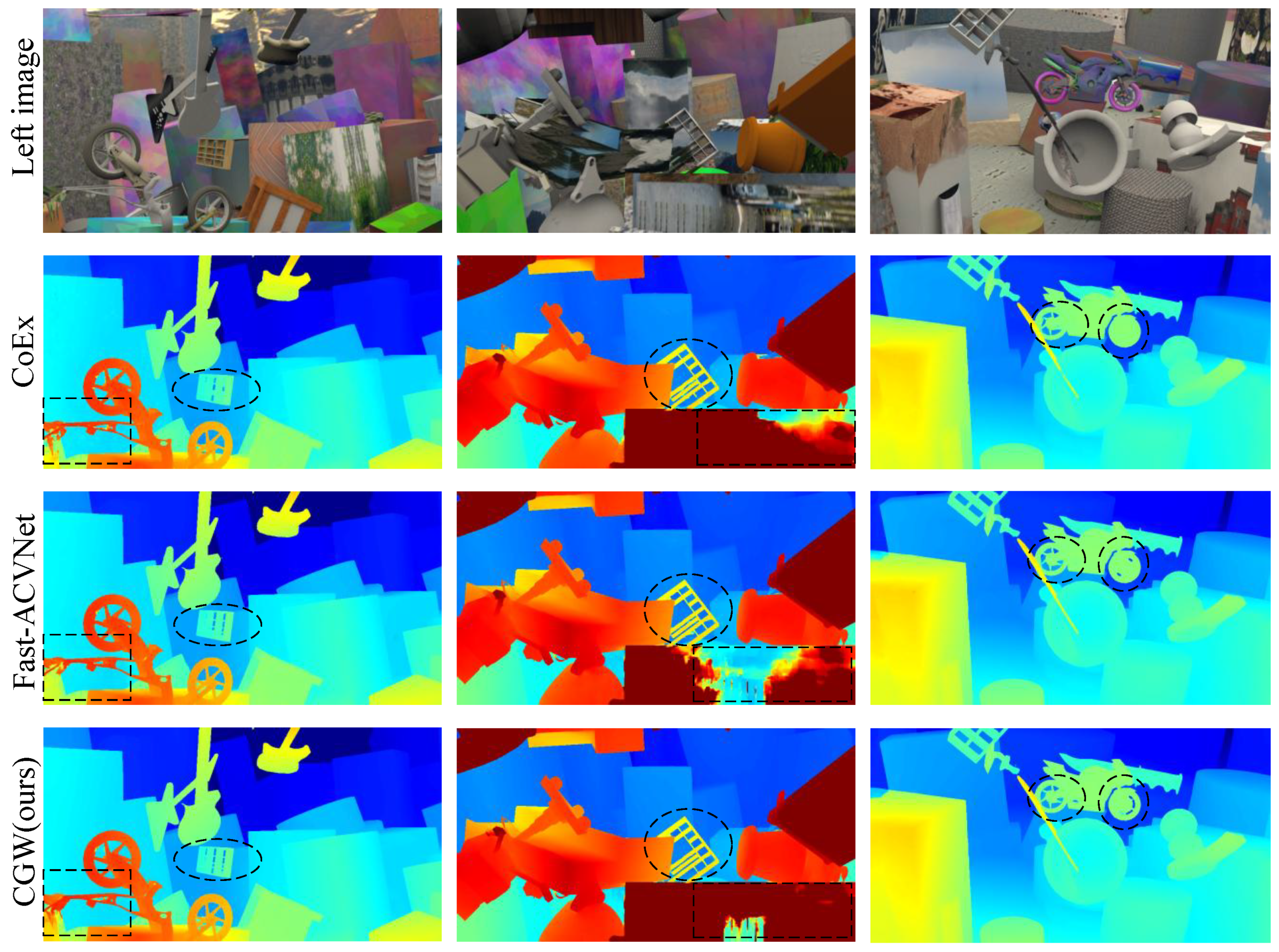
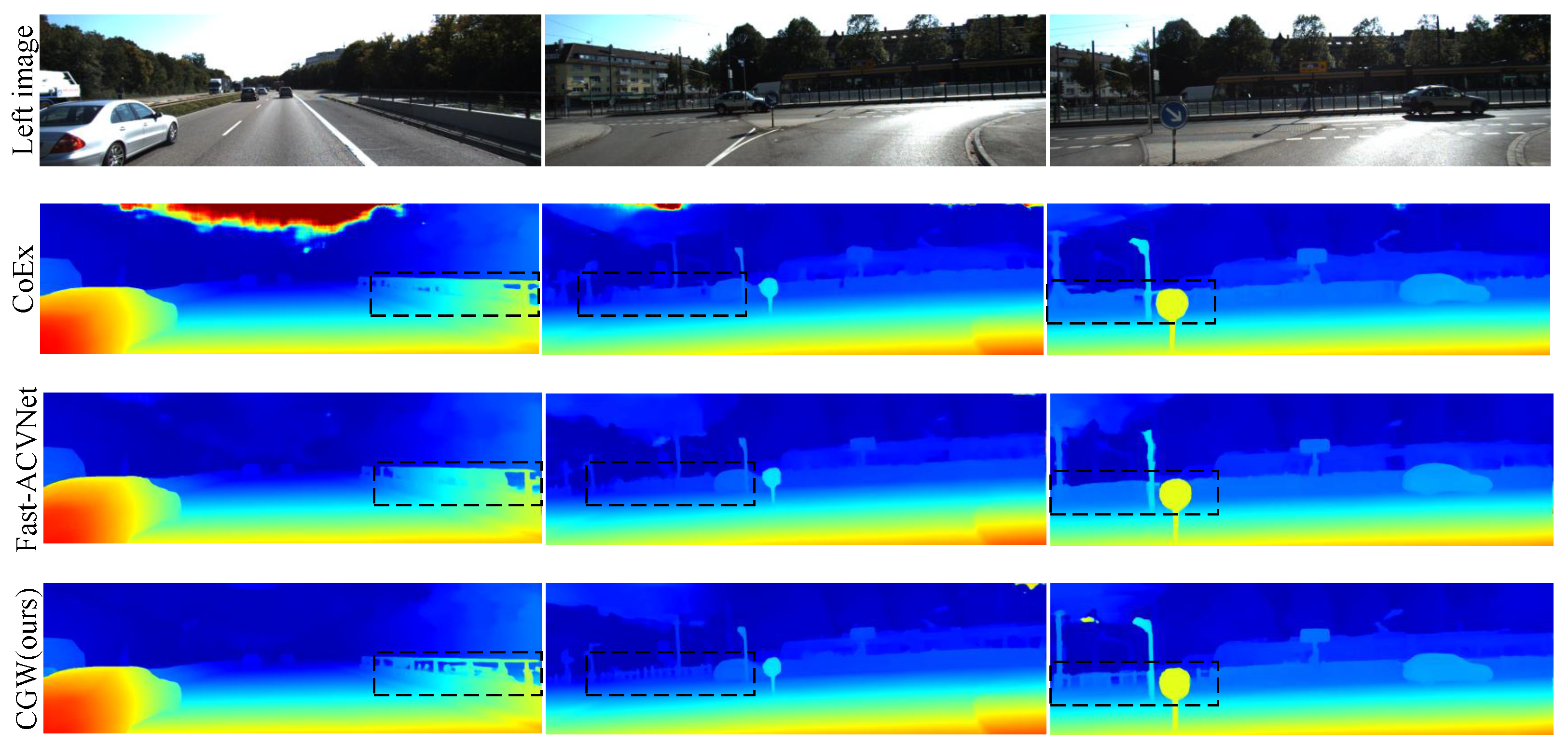
4.5. Generalization Performance

Due to the sufficient quantity of data in the Scene Flow dataset, most stereo matching models demonstrated outstanding performance on this dataset. For different datasets, we fine-tuned the model to obtain the best model for each dataset. At the same time, due to our model’s use of the CGA module and attention weights to cascade contextual and geometric information, the handling of detailed information was well executed, which greatly enhanced the model’s generalization ability. For an assessment of the generalization ability, we tested our model and other great models trained only on the Scene Flow dataset on multiple different datasets. The results are displayed in

Table 5. Comparing the generalization ability of different top-performing models on Scene Flow [13]. Bold: Best.

Model	Middlebury	KITTI2012	KITTI2015	ETH3D
	Bad 2.0	D1-all	D1-all	Bad 1.0
	(%)	(%)	(%)	(%)
GANet [7]	20.3	10.1	11.7	14.1
CFNet [36]	15.4	5.1	6.0	5.3
PSMNet [4]	15.8	6.0	6.3	9.8
DSMNet [44]	13.8	6.2	6.5	6.2
STTR [45]	15.5	8.7	6.7	17.2
RAFT-Stereo [29]	12.6	-	5.7	3.3
DeepPrunerFast [6]	38.7	16.8	15.9	36.8
BGNet [22]	24.7	24.8	20.1	22.6
CoEx [10]	25.5	13.5	11.6	9.0
CGI-Stereo [11]	13.5	6.0	5.8	6.3
Fast-ACV [12]	20.1	12.4	10.6	8.1
CGW (ours)	11.3	5.8	5.5	5.9

. Our CGW achieved better generalization performance. Qualitative results are displayed in Figure 7, which shows that our method demonstrated significant generalization capabilities.

5. Conclusions

In this paper, we described how we designed the CGW stereo matching model, which achieves outstanding performance in both its runtime and accuracy compared to other advanced models, while also significantly improving the generalization performance. We introduced depthwise separable convolutions with residual structures into feature extraction and the 3D regularization network, greatly reducing the network’s computational complexity and computation time while maintaining high accuracy. Based on the real-time model, we designed the CGA and WDR modules to improve the model’s accuracy. During feature extraction, we extracted contextual features and geometric information from the cost volume, which were then fused and fed into the cost aggregation to obtain more accurate and effective context attention for enriching the cost volume information. Additionally, for the initial disparity, we used left features, the 4D warping volume, the initial disparity, and the reconstruction error to guide the optimization of the disparity map, further improving the accuracy. By combining CGA and WDF, we minimally reduced the computational speed, ensuring that the overall network maintained high competitiveness in terms of its accuracy, runtime, and generalization capability. Consequently, our network strikes an excellent balance between accuracy and the runtime.

References

1. Kong, D.; Tao, H. A method for learning matching errors for stereo computation. In Proceedings of the British Machine Vision Conference, Kingston, UK, 7–9 September 2004; Volume 1, p. 2. [Google Scholar]
2. Zbontar, J.; LeCun, Y. Stereo matching by training a convolutional neural network to compare image patches. J. Mach. Learn. Res. 2016, 17, 1–32. [Google Scholar]
3. Kendall, A.; Martirosyan, H.; Dasgupta, S.; Henry, P.; Kennedy, R.; Bachrach, A.; Bry, A. End-to-end learning of geometry and context for deep stereo regression. In Proceedings of the IEEE International Conference on Computer Vision, Venice, Italy, 22–29 October 2017; pp. 66–75. [Google Scholar]
4. Chang, J.R.; Chen, Y.S. Pyramid stereo matching network. In Proceedings of the IEEE Conference on Computer Vision and Pattern Recognition, Salt Lake City, UT, USA, 18–22 June 2018; pp. 5410–5418. [Google Scholar]
5. Guo, X.; Yang, K.; Yang, W.; Wang, X.; Li, H. Group-wise correlation stereo network. In Proceedings of the IEEE/CVF Conference on Computer Vision and Pattern Recognition, Long Beach, CA, USA, 15–20 June 2019; pp. 3273–3282. [Google Scholar]
6. Duggal, S.; Wang, S.; Ma, W.C.; Hu, R.; Urtasun, R. Deeppruner: Learning efficient stereo matching via differentiable patchmatch. In Proceedings of the IEEE/CVF International Conference on Computer Vision, Seoul, Republic of Korea, 27 October–2 November 2019; pp. 4384–4393. [Google Scholar]
7. Zhang, F.; Prisacariu, V.; Yang, R.; Torr, P.H. Ga-net: Guided aggregation net for end-to-end stereo matching. In Proceedings of the IEEE/CVF Conference on Computer Vision and Pattern Recognition, Seoul, Republic of Korea, 27 October–2 November 2019; pp. 185–194. [Google Scholar]
8. Imtiaz, S.M.; Kwon, K.C.; Hossain, M.B.; Alam, M.S.; Jeon, S.H.; Kim, N. Depth estimation for integral imaging microscopy using a 3D–2D CNN with a weighted median filter. Sensors 2022, 22, 5288. [Google Scholar] [CrossRef]
9. Xu, H.; Zhang, J. Aanet: Adaptive aggregation network for efficient stereo matching. In Proceedings of the IEEE/CVF Conference on Computer Vision and Pattern Recognition, Seattle, WA, USA, 13–19 June 2020; pp. 1959–1968. [Google Scholar]
10. Bangunharcana, A.; Cho, J.W.; Lee, S.; Kweon, I.S.; Kim, K.S.; Kim, S. Correlate-and-excite: Real-time stereo matching via guided cost volume excitation. In Proceedings of the 2021 IEEE/RSJ International Conference on Intelligent Robots and Systems (IROS), Prague, Czech Republic, 27 September–1 October 2021; pp. 3542–3548. [Google Scholar]
11. Luo, W.; Lu, Z.; Liao, Q. LNMVSNet: A Low-Noise Multi-View Stereo Depth Inference Method for 3D Reconstruction. Sensors 2024, 24, 2400. [Google Scholar] [CrossRef]
12. Xu, G.; Wang, Y.; Cheng, J.; Tang, J.; Yang, X. Accurate and efficient stereo matching via attention concatenation volume. IEEE Trans. Pattern Anal. Mach. Intell. 2023, 46, 2461–2474. [Google Scholar] [CrossRef] [PubMed]
13. Mayer, N.; Ilg, E.; Hausser, P.; Fischer, P.; Cremers, D.; Dosovitskiy, A.; Brox, T. A large dataset to train convolutional networks for disparity, optical flow, and scene flow estimation. In Proceedings of the IEEE Conference on Computer Vision and Pattern Recognition, Las Vegas, NV, USA, 27–30 June 2016; pp. 4040–4048. [Google Scholar]
14. Li, X.; Zhang, C.; Su, W.; Tao, W. IINet: Implicit Intra-inter Information Fusion for Real-Time Stereo Matching. In Proceedings of the AAAI Conference on Artificial Intelligence, Vancouver, BC, Canada, 20–27 February 2024; Volume 38, pp. 3225–3233. [Google Scholar]
15. Xu, G.; Cheng, J.; Guo, P.; Yang, X. Attention concatenation volume for accurate and efficient stereo matching. In Proceedings of the IEEE/CVF Conference on Computer Vision and Pattern Recognition, New Orleans, LA, USA, 18–24 June 2022; pp. 12981–12990. [Google Scholar]
16. Smolyanskiy, N.; Kamenev, A.; Birchfield, S. On the importance of stereo for accurate depth estimation: An efficient semi-supervised deep neural network approach. In Proceedings of the IEEE Conference on Computer Vision and Pattern Recognition Workshops, Salt Lake City, UT, USA, 18–22 June 2018; pp. 1007–1015. [Google Scholar]
17. Chang, J.R.; Chang, P.C.; Chen, Y.S. Attention-aware feature aggregation for real-time stereo matching on edge devices. In Proceedings of the Asian Conference on Computer Vision, Kyoto, Japan, 30 November–4 December 2020. [Google Scholar]
18. Tankovich, V.; Hane, C.; Zhang, Y.; Kowdle, A.; Fanello, S.; Bouaziz, S. Hitnet: Hierarchical iterative tile refinement network for real-time stereo matching. In Proceedings of the IEEE/CVF Conference on Computer Vision and Pattern Recognition, Nashville, TN, USA, 20–25 June 2021; pp. 14362–14372. [Google Scholar]
19. Shamsafar, F.; Woerz, S.; Rahim, R.; Zell, A. Mobilestereonet: Towards lightweight deep networks for stereo matching. In Proceedings of the IEEE/CVF Winter Conference on Applications of Computer Vision, Waikoloa, HI, USA, 3–8 January 2022; pp. 2417–2426. [Google Scholar]
20. Yee, K.; Chakrabarti, A. Fast deep stereo with 2D convolutional processing of cost signatures. In Proceedings of the IEEE/CVF Winter Conference on Applications of Computer Vision, Snowmass Village, CO, USA, 1–5 March 2020; pp. 183–191. [Google Scholar]
21. Khamis, S.; Fanello, S.; Rhemann, C.; Kowdle, A.; Valentin, J.; Izadi, S. Stereonet: Guided hierarchical refinement for real-time edge-aware depth prediction. In Proceedings of the European Conference on Computer Vision (ECCV), Munich, Germany, 8–14 September 2018; pp. 573–590. [Google Scholar]
22. Möckl, L.; Roy, A.R.; Petrov, P.N.; Moerner, W. Accurate and rapid background estimation in single-molecule localization microscopy using the deep neural network BGnet. Proc. Natl. Acad. Sci. USA 2020, 117, 60–67. [Google Scholar] [CrossRef] [PubMed]
23. Zeng, J.; Yao, C.; Yu, L.; Wu, Y.; Jia, Y. Parameterized cost volume for stereo matching. In Proceedings of the IEEE/CVF International Conference on Computer Vision, Paris, France, 2–6 October 2023; pp. 18347–18357. [Google Scholar]
24. Zhong, Y.; Loop, C.; Byeon, W.; Birchfield, S.; Dai, Y.; Zhang, K.; Kamenev, A.; Breuel, T.; Li, H.; Kautz, J. Displacement-invariant cost computation for stereo matching. Int. J. Comput. Vis. 2022, 130, 1196–1209. [Google Scholar] [CrossRef]
25. Zhang, S.; Wang, Z.; Wang, Q.; Zhang, J.; Wei, G.; Chu, X. Ednet: Efficient disparity estimation with cost volume combination and attention-based spatial residual. In Proceedings of the IEEE/CVF Conference on Computer Vision and Pattern Recognition, Nashville, TN, USA, 19–25 June 2021; pp. 5433–5442. [Google Scholar]
26. Liang, Z.; Guo, Y.; Feng, Y.; Chen, W.; Qiao, L.; Zhou, L.; Zhang, J.; Liu, H. Stereo matching using multi-level cost volume and multi-scale feature constancy. IEEE Trans. Pattern Anal. Mach. Intell. 2019, 43, 300–315. [Google Scholar] [CrossRef] [PubMed]
27. Zhao, H.; Zhou, H.; Zhang, Y.; Chen, J.; Yang, Y.; Zhao, Y. High-frequency stereo matching network. In Proceedings of the IEEE/CVF Conference on Computer Vision and Pattern Recognition, Vancouver, BC, Canada, 18–22 June 2023; pp. 1327–1336. [Google Scholar]
28. Shen, Z.; Dai, Y.; Song, X.; Rao, Z.; Zhou, D.; Zhang, L. Pcw-net: Pyramid combination and warping cost volume for stereo matching. In Proceedings of the European Conference on Computer Vision, Tel Aviv, Israel, 23–27 October 2022; Springer: Cham, Switzerland, 2022; pp. 280–297. [Google Scholar]
29. Lipson, L.; Teed, Z.; Deng, J. Raft-stereo: Multilevel recurrent field transforms for stereo matching. In Proceedings of the 2021 International Conference on 3D Vision (3DV), London, UK, 1–3 December 2021; pp. 218–227. [Google Scholar]
30. Xu, G.; Wang, X.; Ding, X.; Yang, X. Iterative geometry encoding volume for stereo matching. In Proceedings of the IEEE/CVF Conference on Computer Vision and Pattern Recognition, Vancouver, BC, Canada, 18–22 June 2023; pp. 21919–21928. [Google Scholar]
31. Wang, X.; Xu, G.; Jia, H.; Yang, X. Selective-stereo: Adaptive frequency information selection for stereo matching. In Proceedings of the IEEE/CVF Conference on Computer Vision and Pattern Recognition, Seattle, WA, USA, 17–21 June 2024; pp. 19701–19710. [Google Scholar]
32. He, K.; Zhang, X.; Ren, S.; Sun, J. Deep residual learning for image recognition. In Proceedings of the IEEE Conference on Computer Vision and Pattern Recognition, Las Vegas, NV, USA, 27–30 June 2016; pp. 770–778. [Google Scholar]
33. Szegedy, C.; Liu, W.; Jia, Y.; Sermanet, P.; Reed, S.; Anguelov, D.; Erhan, D.; Vanhoucke, V.; Rabinovich, A. Going deeper with convolutions. In Proceedings of the IEEE Conference on Computer Vision and Pattern Recognition, Boston, MA, USA, 7–12 June 2015; pp. 1–9. [Google Scholar]
34. Howard, A.; Sandler, M.; Chu, G.; Chen, L.C.; Chen, B.; Tan, M.; Wang, W.; Zhu, Y.; Pang, R.; Vasudevan, V.; et al. Searching for mobilenetv3. In Proceedings of the IEEE/CVF International Conference on Computer Vision, Seoul, Republic of Korea, 27 October–2 November 2019; pp. 1314–1324. [Google Scholar]
35. Yang, F.; Sun, Q.; Jin, H.; Zhou, Z. Superpixel segmentation with fully convolutional networks. In Proceedings of the IEEE/CVF Conference on Computer Vision and Pattern Recognition, Seattle, WA, USA, 14–19 June 2020; pp. 13964–13973. [Google Scholar]
36. Shen, Z.; Dai, Y.; Rao, Z. Cfnet: Cascade and fused cost volume for robust stereo matching. In Proceedings of the IEEE/CVF Conference on Computer Vision and Pattern Recognition, Nashville, TN, USA, 19–25 June 2021; pp. 13906–13915. [Google Scholar]
37. Sandler, M.; Howard, A.; Zhu, M.; Zhmoginov, A.; Chen, L.C. Mobilenetv2: Inverted residuals and linear bottlenecks. In Proceedings of the IEEE Conference on Computer Vision and Pattern Recognition, Salt Lake City, UT, USA, 18–22 June 2018; pp. 4510–4520. [Google Scholar]
38. Geiger, A.; Lenz, P.; Urtasun, R. Are we ready for autonomous driving? The kitti vision benchmark suite. In Proceedings of the 2012 IEEE Conference on Computer Vision and Pattern Recognition, Providence, RI, USA, 16–21 June 2012; pp. 3354–3361. [Google Scholar]
39. Menze, M.; Geiger, A. Object scene flow for autonomous vehicles. In Proceedings of the IEEE Conference on Computer Vision and Pattern Recognition, Boston, MA, USA, 7–12 June 2015; pp. 3061–3070. [Google Scholar]
40. Scharstein, D.; Hirschmüller, H.; Kitajima, Y.; Krathwohl, G.; Nešić, N.; Wang, X.; Westling, P. High-resolution stereo datasets with subpixel-accurate ground truth. In Proceedings of the Pattern Recognition: 36th German Conference, GCPR 2014, Münster, Germany, 2–5 September 2014; Proceedings 36. Springer: Berlin/Heidelberg, Germany, 2014; pp. 31–42. [Google Scholar]
41. Schops, T.; Schonberger, J.L.; Galliani, S.; Sattler, T.; Schindler, K.; Pollefeys, M.; Geiger, A. A multi-view stereo benchmark with high-resolution images and multi-camera videos. In Proceedings of the IEEE Conference on Computer Vision and Pattern Recognition, Honolulu, HI, USA, 21–26 July 2017; pp. 3260–3269. [Google Scholar]
42. Kingma, D.P.; Ba, J. Adam: A method for stochastic optimization. arXiv 2014, arXiv:1412.6980. [Google Scholar]
43. Cheng, X.; Zhong, Y.; Harandi, M.; Dai, Y.; Chang, X.; Li, H.; Drummond, T.; Ge, Z. Hierarchical neural architecture search for deep stereo matching. Adv. Neural Inf. Process. Syst. 2020, 33, 22158–22169. [Google Scholar]
44. Zhang, F.; Qi, X.; Yang, R.; Prisacariu, V.; Wah, B.; Torr, P. Domain-invariant stereo matching networks. In Proceedings of the Computer Vision–ECCV 2020: 16th European Conference, Glasgow, UK, 23–28 August 2020; Proceedings, Part II 16. Springer: Berlin/Heidelberg, Germany, 2020; pp. 420–439. [Google Scholar]
45. Li, Z.; Liu, X.; Drenkow, N.; Ding, A.; Creighton, F.X.; Taylor, R.H.; Unberath, M. Revisiting stereo depth estimation from a sequence-to-sequence perspective with transformers. In Proceedings of the IEEE/CVF International Conference on Computer Vision, Montreal, QC, Canada, 11–17 October 2021; pp. 6197–6206. [Google Scholar]
Figure 1. The model of the CGW. It extracts multi-scale features and constructs the cost volume using 1/4-scale features. The cost aggregation is performed through a 3D regularization network and context geometry attention (CGA), which the generates context geometry attention volume. These weights filter the context features to create the context geometry volume and obtain the initial disparity. Finally, the Warping Disparity Refinement module (WDR) was applied to further optimize the disparity.
Electronics 14 00892 g001
Figure 2. The architecture of the 3D separable convolution with a residual structure.
Electronics 14 00892 g002
Figure 3. The architecture of context geometry attention (CGA).
Electronics 14 00892 g003
Figure 4. The architecture of Warping Disparity Refinement.
Electronics 14 00892 g004
Figure 5. Visual comparison of results on Scene Flow.
Electronics 14 00892 g005
Figure 6. Visual comparisons with other methods on KITTI 2012 [38] and 2015 [39] test sets.
Electronics 14 00892 g006
Figure 7. Visual generalization results on Middlebury 2014 and ETH3D.
Electronics 14 00892 g007