Abstract
In recent wind power forecasting studies, deep neural networks have shown powerful performance in estimating future power from wind power data. In this paper, a pseudo-twin neural network model of full multi-layer perceptron is proposed for power forecasting in wind farms. In this model, the input wind power data are divided into physical attribute data and historical power data. These two types of input data are processed separately by the feature extraction module of the pseudo-twin structure to obtain physical attribute features and historical power features. To ensure comprehensive integration and establish a connection between the two types of extracted features, a feature mixing module is introduced to cross-mix the features. After mixing, a set of multi-layer perceptrons is used as a power regression module to forecast wind power. In this paper, simulation research is carried out based on measured data. The proposed model is compared with mainstream models such as CNN, RNN, LSTM, GRU, and hybrid neural network. The results show that the MAE and RMSE of the single-step forecasting of the proposed model are reduced by up to 21.88% and 16.85%, respectively. Additionally, the MAE and RMSE of the 1 h rolling forecasting (six steps ahead) are reduced by up to 31.58% and 40.92%, respectively.
1. Introduction
As a renewable energy source, wind energy can replace fossil fuels to reduce carbon emissions and alleviate global warming. However, wind energy is inherently uncertain, and wind power can fluctuate significantly in a short period, affecting the safe and stable operation of the power grid. Therefore, improving the accuracy of wind power forecasting has become a hot research topic [1,2].
Currently, ultra-short-term wind power forecasting methods are primarily divided into three categories: physical models based on high-dimensional mathematical equations, statistical methods based on time series analysis, and data-driven machine learning methods. Among these, physical models [3] and statistical methods [4] were introduced in the early stages of wind power forecasting. The former forecasts wind power by establishing mathematical relationship models between meteorological factors and wind power, but its drawback lies in its heavy reliance on meteorological data and physical principles. The latter forecasts wind power by establishing mapping relationships between historical data and wind power through probabilistic autoregression models [5], probabilistic quality deviation models [6], and auto-regressive models [7,8]. However, these models lack sufficient nonlinear capabilities and are unable to handle the irregular and nonlinear characteristics of wind power sequences. With the advancement of intelligent computing, data-driven machine learning methods have been applied to the field of wind power forecasting. These methods process various types of data, including power and meteorological data, to extract and select features that can reflect future power changes. By correlating power variations with external factors, they achieve high-accuracy forecasting.
Machine learning methods applied to power forecasting mainly include traditional machine learning methods and deep learning models. Traditional machine learning methods rely on feature engineering and have limited capabilities in handling high-dimensional data and complex patterns. In contrast, deep learning models can directly pass data through the network, extracting features to establish correlations between power and various factors, thereby achieving high-accuracy forecasting. The research in the reference [9] proves this point.
Typical deep learning methods include ANNs (artificial neural networks), CNNs (convolutional neural networks), RNNs (recurrent neural networks), and their variants. Reference [10] proposed a BP-ANN model for short-term wind power forecasting. However, the nonlinear learning ability of traditional artificial neural networks is limited. The research in reference [11] shows that the forecasting accuracy of CNNs can be improved by 11.09% compared with BP. But CNNs can only capture dependencies between short-term data. In order to improve the forecasting accuracy of wind power, the sequence model is introduced into the task as a new forecasting technology. There are recursive links in the network structure, which can learn the relationship between the samples. The research in reference [12] proves this point. Compared with CNNs, the MAE (mean absolute error) of RNNs is reduced by 11.44%. As an improved version of RNNs, LSTM (Long Short-Term Memory) aims to solve the common long-term dependence problem in RNNs by combining short-term and long-term memory through gating [13]. GRU (Gate Recurrent Unit) is an optimized structure of LSTM, which simplifies the model and improves the forecasting accuracy. The research in reference [14] shows that the forecasting of the GRU model can be improved by 16.57% compared with LSTM, and the training time is only two-thirds of the former. In addition, in order to capture the high-dimensional features in the wind power dataset, a hybrid neural network is developed. References [12,15] have proven the superiority of the hybrid neural network compared to a single forecasting model.
In addition to the deep learning models mentioned above, some models have been applied well in time series forecasting in other fields. These models also have great application potential in wind power forecasting. Reference [16] used multi-layer perceptron to forecast the hourly power generation capacity of 16 photovoltaic power stations in northern Italy. Reference [17] constructed a TCM model based on MLP and verified the effectiveness of the model in weather, disease, transportation, and other fields. Reference [18] constructed a model based on MLP to simulate the humidity change in minerals and forecast the drying degree of materials. The above research shows that MLP has been applied to different fields and performs various tasks. Therefore, the improved model based on MLP can forecast wind power well.
Although these models have made progress, it is still very challenging to obtain satisfactory wind power forecasting results using deep learning models due to the non-stationary characteristics of meteorological factors. Inspired by some multi-channel models, such as reference [19], multi-scale network hybrid meteorological feature power characteristics are established to improve the forecasting accuracy of photovoltaic power. Reference [20] established a new multi-branch deep neural network, which uses multiple branches to extract different information and correlations in the input data to improve the accuracy of fault diagnosis. The above research shows that the forecasting accuracy can be improved by multi-view feature extraction. Therefore, combined with the above, the model based on MLP and multi-view feature extraction is expected to achieve higher forecasting accuracy.
In this paper, a pseudo-twin neural network based on full multi-layer perceptron is proposed for wind power forecasting. The model makes full use of meteorological data and historical power data to extract and fuse features, which makes the ultra-short-term wind power forecasting results reliable. The forecasting accuracy of the model is verified by the measured data. The results show that the forecasting accuracy of the proposed model is higher than that of other baseline models.
The main innovations and contributions of this paper are as follows:
- (1)
- Multi-view feature extraction. The input data are divided into physical attribute data and historical power data. The neural network of the pseudo-twin structure is designed to extract the features of physical attribute data and historical power data, respectively.
- (2)
- Construct a full MLP neural network for wind power forecasting. Based on MLP, relevant modules are constructed to extract and fuse features to improve the nonlinear expression ability of the model.
2. Forecasting Model Design and Implementation
2.1. Model Structure
As shown in Figure 1, the proposed model consists of a pseudo-twin feature extraction module, a feature mixing module, and a power regression module. The basic forecasting process is as follows. First, the wind power data are divided into physical attribute data and historical power data, and then these two types of data are sent into the pseudo-twin feature extraction module to obtain the physical attribute features and historical power features of wind power. Next, the feature mixing module is used to fuse the two types of features extracted. Finally, the mixed features are reconstructed and sent to a set of multi-layer perceptrons to perform power regression. The process described above is a single-step forecasting of wind power. To achieve multi-step forecasting, you can use the power forecasting result at the previous time step as the historical power of the power forecasting at the next moment to perform iterative forecasting.
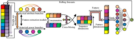
Figure 1.
The overall architecture of the model.
2.2. Pseudo-Twin Feature Extraction Module
In some recent studies on wind power forecasting, most deep learning models integrate different types of data as model input, and then design a backbone network to extract features for power forecasting. However, this approach does not account for the fact that different types of networks have different representation capabilities for different types of data. In addition to considering the compatibility between the network and the data, the mixing of different dimensional data to extract features will also limit the expression ability of the network, making it difficult for the network to focus on specific types of feature representation. Therefore, in this paper, the feature extraction module of the pseudo-twin structure is constructed by breaking away from the design approach of previous models. The module includes a physical attribute branch and a historical power branch, which process physical attribute data and historical power data, respectively, so that the features are fully expressed.
2.2.1. Multi-Layer Perceptron
In the current deep learning model for wind power forecasting, convolutional neural networks and sequence models are widely used to extract local high-dimensional features and long-term trends in wind power data. However, there are fewer and fewer research reports on wind power forecasting models based on artificial neural networks. Compared with convolution and sequence models, artificial neural networks have stronger nonlinear expression ability. However, there are some defects in the artificial neural network; namely, when the number of layers is too shallow, the nonlinear expression ability is insufficient, and when the network is too deep, the model is difficult to converge, and there are problems of gradient vanishing and gradient explosion.
In order to solve the above problems, this paper draws inspiration from traditional artificial neural networks and improves upon them. An artificial neural network that conforms to wind power forecasting is designed, which is also called multi-layer perceptron. The multi-layer perceptron designed in this paper is shown in Figure 2. There are two fully connected layers in each group of multi-layer perceptrons. In other words, the simplest structure of the multi-layer perceptron designed in this paper (not the simplest structure of the artificial neural network, the artificial neural network without a hidden layer is called a single-layer perceptron) contains only one hidden layer. This is due to the fact that the design of multiple hidden layers will hinder the reverse propagation of the gradient, which is also the design disadvantage of the traditional artificial neural network.
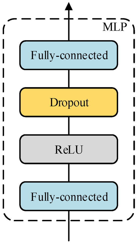
Figure 2.
The structure of MLP.
In all the multi-layer perceptron designs in this paper, whether they are used for sequence expansion or residual learning, an anti-bottleneck structure is adopted. This structure can make the feature transition from small dimensions to large dimensions and then back to small dimensions. The number of neurons in the hidden layer is r times that of the output layer, thus avoiding compression loss when information is transformed in different dimension spaces. In addition, considering that the extensive use of the fully connected layer will lead to the problem that the model is difficult to converge, a dropout layer is added after the first fully connected layer in the multi-layer perceptron to randomly deactivate neurons, solve the convergence problem, and prevent network overfitting.
2.2.2. Feature Extraction Branches
A single multi-layer perceptron cannot meet the nonlinear requirements of wind power forecasting tasks. To address this, this paper constructs a deep neural network based on the designed multi-layer perceptron to process the data.
As shown in Figure 3, the specific structure of the physical property branch in the feature extraction module is shown. Since the designed feature extraction module is a pseudo-twin mechanism, the network structure of the physical property branch is exactly the same as that of the historical power branch. Therefore, in this section, the physical property branch is introduced in detail as an example.
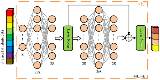
Figure 3.
The structure of the feature extraction branch.
As can be seen from Figure 3, the feature extraction branch consists of MLP-E (Multi-layer Perceptron Extractor), which contains two multi-layer perceptrons. Among them, the first multi-layer perceptron is used for sequence expansion and for transforming a sequence with an original length of S into a sequence of length 2S. The second multi-layer perceptron is used as the residual block. The number of neurons in the input layer and the output layer is consistent, and the sequence length is maintained. The output features of the second multi-layer perceptron are added to the output features of the first multi-layer perceptron for residual learning. The purpose of this is to increase the depth of the network and improve the nonlinear expression ability of the model. At the same time, it avoids issues such as model convergence difficulties and volatile forecasting results due to the extensive use of the fully connected layer. In addition, a normalization layer is added after each multi-layer perceptron to prevent gradient vanishing.
In particular, in the feature extraction branch designed in this paper, N groups of MLP-E can be cascaded. The output features of each group of MLP-E can be used as the input features of the next group of MLP-E to realize the step-by-step expansion of the sequence dimension. The length of the expanded sequence is twice that before expansion.
2.3. Feature Mixture and Power Regression
In the wind power forecasting model, most networks will directly use artificial neural networks to forecast wind power after extracting features. However, in the pseudo-twin neural network, since the physical attribute features and historical power features are extracted separately, there is a lack of sufficient coupling between the two types of features. If the wind power is directly regressed by the artificial neural network, the forecasting accuracy will be significantly affected. Therefore, this paper introduces a new module in the model design between the feature extraction module and the power regression, which is called the feature mixing module. Its purpose is to establish the coupling relationship between the physical attribute features and the historical power features.
The specific structure of the feature mixing module is shown in Figure 4. It can be observed that the core component of the module is MLP-M (Multi-layer Perceptron Mixer), and the specific structure is the selected part of the purple dotted frame in the figure. In this mixer, there are two multi-layer perceptrons. Among them, the first multi-layer perceptron is used for dimension expansion to initially mix features, and the second multi-layer perceptron is used to compress the dimension to make the dimension size consistent with the size before mixing.
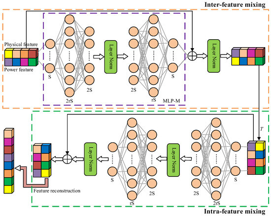
Figure 4.
The structure of the feature mixing module.
The specific steps of feature mixing are as follows. The features from the pseudo-twin feature extraction module are simply spliced in the feature dimension. However, the fusion method of this feature is hard fusion, which only changes the feature dimension without establishing information coupling. Therefore, the spliced features are mixed on the feature dimension through MLP-M, and the skip connection is used to form a residual structure with MLP-M to form feature-to-feature learning of physical attributes and historical power. Similarly, the results of each case of residual learning are normalized to obtain the mixed features. In addition to mixing the feature dimensions to form inter-feature mixing, it is also necessary to mix the sequence dimensions to construct the coupling relationship within the features and form intra-feature mixing. Therefore, inspired by reference [21], it is necessary to perform transpose operations (the symbol T is in Figure 4) on the features after inter-feature mixing, exchange dimensions, and perform the same mixing operations before again mixing sequence dimensions and mining information relationships within features.
The inter-feature mixing and intra-feature mixing make the features from the pseudo-twin feature extraction module cross-mixed, and the mixed features can be used for power regression. This paper will reconstruct the features after cross-mixing, folded along the dimensions, and use a set of multi-layer perceptrons to achieve power regression.
3. Simulation Settings
3.1. The Program Steps of the Proposed Method
The forecasting process is shown in Figure 5, as follows:
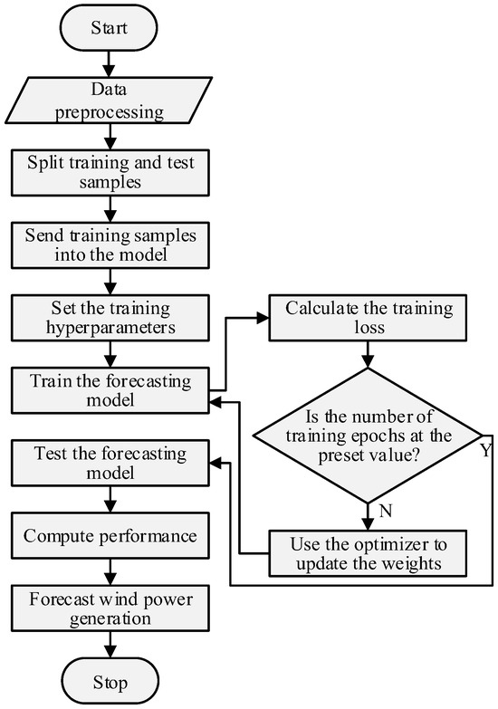
Figure 5.
Forecasting flow chart.
Step 1: Data preprocessing
- (1)
- Load the original wind power data; divide the training samples and test samples.
- (2)
- Fill the vacancy data, then perform data normalization.
Step 2: Training the model
- (1)
- Set the training hyperparameters, such as the number of training rounds, the number of batch training samples, and the learning rate.
- (2)
- Send the training sample data into the model, calculate the training loss, and use the optimizer algorithm to update the model weight until the epoch reaches the preset hyperparameter value.
Step 3: Forecasting and computational performance
- (1)
- Use the model trained in step 2 to forecast the test sample data.
- (2)
- Denormalize the forecasting results, and calculate the validity of the model according to the performance index.
3.2. Loss Function
The loss function is an important part of the deep learning model. The forecasting ability of the model is estimated by the obtained real value and the model forecasting value to show that the current model can be effectively used for forecasting tasks. When the loss value is large, it indicates that the forecasting ability of the model is insufficient; when the loss value is small, it shows that the model has been trained sufficiently to carry out the forecasting task. The loss function used in this paper is the mean square error (MSE), which is sensitive to large forecasting deviation and can improve the stability of forecasting models:
In the formula, n is the number of samples, is the actual wind power, and is the forecasting wind power.
3.3. Performance Indicators
MAE refers to the mean absolute error between the forecasted value and the actual value. Because it calculates the absolute value, it can avoid the offset of positive and negative values and reflect the overall level of model forecasting. The smaller the MAE, the higher the forecasting accuracy:
RMSE represents the sample standard deviation of the forecasting error, that is, the degree of dispersion of the forecasting error. When the RMSE is larger, it indicates that the model forecasting is more unstable:
4. Case Study 1
In this section, the effectiveness of the wind power forecasting method proposed in this paper is proved by simulation. Firstly, the hyperparameters of the model are adjusted based on the grid search method to optimize the performance of the proposed ultra-short-term wind power forecasting model. In the process of parameter adjustment, the box plot is used to show the verification loss of the model under different parameters after each adjustment, so as to prove the validity of the model parameter adjustment. Then, the performance of the proposed model is compared with the current mainstream methods, such as the CNNs, RNNs, LSTM, GRU, and hybrid neural networks of these models. Of course, for these mainstream methods, this paper also uses the grid search method to ensure the fairness of the comparison.
The training and forecasting of all models are implemented on a personal computer’s graphics processing unit (GPU) with 2GB video memory, 16GB RAM and Intel Core i5’s central processing unit (CPU), using python 3.7 software and based on the Pytorch deep learning framework.
4.1. Dataset
The wind power data used in this case study were collected from northwest China, including five wind turbines. The rated power of a single wind turbine is 1.5 MW. Each wind turbine contains an independent data acquisition system, which can independently record physical attribute data such as wind speed and wind direction and historical power data. The sampling resolution is 10 min. The input physical attribute data and historical data are shown in Table 1.

Table 1.
Data list of Case 1.
In the process of data acquisition, there may be blank records due to communication and other reasons, resulting in data loss. To solve this problem, in the data processing stage, these vacant data are filled with a value of 0.
4.2. Model Parameter Settings
Different combinations of model parameters will obtain different wind power forecasting results. In this section, the grid search method is used to adjust the hyperparameters in order to obtain the best wind power forecasting results. Although there are many parameters to be adjusted in the training process, including learning rate, batch size, loss function, etc., the following content focuses on the adjustment process of some core parameters related to network design, including the number of MLP-Es and MLP-Ms, the relationship between the number of hidden layer neurons and the number of output layer neurons, and the necessity of the residual module in MLP-E. This paper aims to demonstrate these parameters to illustrate the performance of the proposed model core module, and future researchers can adjust these parameters according to their own task requirements so that the research in this paper can be adapted to their needs.
Because the forecasting results of the deep learning model have a certain randomness (initialization method, training data input order, etc.), each forecasting result is accompanied by certain differences. In view of this, in the parameter adjustment stage, multiple evaluations have been performed on models with different parameters, so that the model does not appear to be skewed by outliers.
In the performance comparison, in order to make the comparison results clearer, the verification loss of multiple forecasting results is shown (since the results are not denormalized, the loss value appears to be too small), and a box plot is used for visualization. At the same time, this paper takes the median of the model forecasting results as the key comparison object, that is, the dotted line in the box plot, which takes into account that the mean value can be influenced by outliers, and the median value is evaluated by the simulation. The number of times is high enough, so it is less affected and more reasonable. Of course, the evaluation process will not take the median value of the model verification loss as the only criterion for model performance. In addition, the maximum value of the verification loss (upper limit of the box plot), the minimum value (lower limit of the box plot), the abnormal value (red data points in the box plot) and the distribution of the verification loss will also be considered.
4.2.1. Selection of the Number of MLP-Es
In the deep learning model, the design and setting of the feature extraction module is very important. If the number of layers is too shallow, the feature extraction is not sufficient, and the model will experience under-fitting. If the number of layers is too deep, the network will have too strong of an expression ability, resulting in over-fitting of the model. Therefore, the appropriate model depth is very important, which can make the features be properly expressed and improve the forecasting accuracy. In the feature extraction module proposed in this paper, MLP-E is designed to extract data features, and the depth of the model is controlled by increasing or decreasing the number of superimposed MLP-Es.
Because the training results of the deep learning model are different each time, there are inherent differences in performance. Therefore, eight simulations are performed on the models under different numbers of MLP-Es to ensure that the proposed model does not appear to have extreme model performance due to accidental forecasting results.
It can be observed from Figure 6 that the median of the model validation loss for all MLP-E numbers fluctuates between the upper and lower quartiles. Initially, this value gradually decreases as the number of MLP-Es increases. However, when the number of MLP-Es is four, the value increases until the number is five, and the value decreases again. Specifically, when the number of MLP-Es is one, the model’s performance is relatively poor, the median validation loss is the highest, and there is a significant outlier. Secondly, when the number of MLP-Es is two and four, the median of the verification loss and the upper and lower limits of the box plot are relatively close in these two cases, and there is no abnormal value. Compared with the number of MLP-Es being five, it has better performance. Although the median of the verification loss is lower when the number of MLP-Es is five, the model’s forecasting stability is insufficient, and the range of the upper and lower limits is the largest. It should be noted that when the number of MLP-Es is three, the forecasting results of the model show strong forecasting robustness. Although there is an outlier in the result, the outlier itself shows good forecasting performance. Therefore, this paper chooses the number of MLP-E as three to improve the forecasting accuracy of the forecasting model.
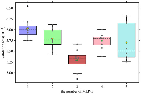
Figure 6.
Validation loss under different numbers of MLP-Es.
From the above research, we can also analyze the conclusion that blindly increasing the depth of the model may not improve the forecasting accuracy of the model, and the forecasting accuracy of the model will be insufficient when the number of network layers is shallow, which verifies that the appropriate model depth is mentioned at the beginning of this section. It is very important to improve the forecasting accuracy.
4.2.2. Selection of the Number of MLP-Ms
In addition to changing the depth of the model by modifying the superposition number of MLP-Es, and then changing the nonlinear expression ability of the model, this paper can also adjust the fusion degree of the features sent by the feature extraction module by modifying the number of MLP-Ms. Since the cross-mixing process requires feature fusion from the sequence dimension and the feature dimension, respectively, two sets of MLP-M are used for a complete cross-fusion. Therefore, when the number of MLP-Ms is selected, the number of MLP-Ms is 0, 2, and 4, respectively, instead of increasing according to the number of steps of 1.
As shown in Figure 7, the forecasting performance of the model under various MLP-M numbers is demonstrated. It can be observed that when the number of MLP-Ms is two, the forecasting performance of the network is the best, and the median line position of the box plot is the lowest. Secondly, when the number of MLP-Ms is 0, although the upper bound of the boxplot is close to that when the number of MLP-M is 2, relatively speaking, most of the verification losses are lower when the number of MLP-M is 2, which also leads to a lower bound of the boxplot at this time, and its average performance is better. Therefore, the number of MLP-M is selected as two.
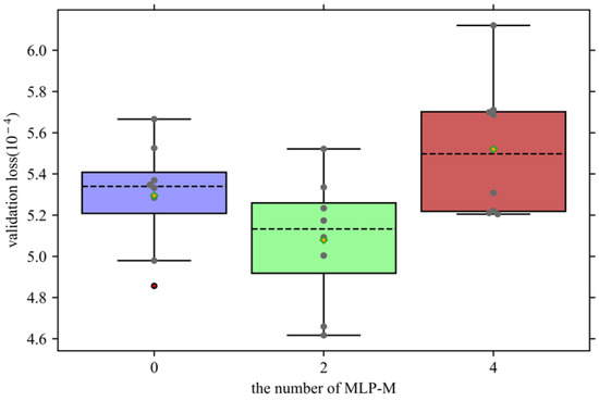
Figure 7.
Validation loss under different numbers of MLP-Ms.
4.2.3. Selection of the Number of Hidden Layer Neurons
In the multi-layer perceptron, in order to adapt the nonlinear expression ability of the model to the current task, this paper achieves this goal by adjusting the number of hidden layer neurons. In general, the number of hidden layer neurons should be a multiple of the number of output layer neurons. Therefore, when designing a multi-layer perceptron, the appropriate number of hidden layer neurons is selected by adjusting the multiple of the number of hidden layer neurons. The verification loss under different multiples of the number of hidden layer neurons is shown in Figure 8.
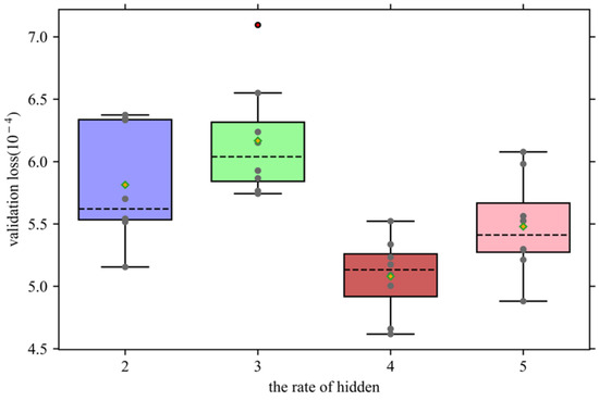
Figure 8.
Validation loss under different numbers of hidden layer neurons.
It can be observed that the performance of the model does not increase with the increase in the number of hidden layer neurons. When the number of hidden layer neurons is two times and three times that of the output layer, the median line of verification loss also increases, and poor forecasting outliers appear. When the multiple is four times that of the output layer, the median line position of the verification loss is the lowest, and the fluctuation of the forecasting is smaller than that of the forecasting result when the multiple is five times larger, and the upper and lower limits of the box plot are lower.
4.2.4. The Necessity of the Residual Module
For MLP-E, this paper increases the depth of the model by adding a residual module to improve the ability of the model. In this simulation, the residual module in the model will be eliminated, and the necessity of the residual module will be verified by verifying the box plot of the loss.
As shown in Figure 9, the verification loss of adding the residual module and not adding the residual module in MLP-Es is shown in the form of a box plot. It can be clearly observed that when the MLP-E does not have an added residual module, the verification loss of the model has a significant increase, which affects the forecasting accuracy.
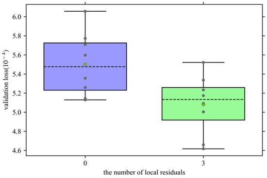
Figure 9.
Validation loss under different numbers of local residual modules.
4.3. Power Forecasting
The wind power data used for power forecasting in this paper is described in detail in Section 4.1. A total of 245 days of data (35,280 samples) were collected for training and testing, of which 90% of the data were used to train the forecasting model and 10% of the data were used to test the effectiveness of the proposed model.
The forecasting model is mainly composed of MLP-E and MLP-M. In the previous chapter, the grid search method is used to determine that the network under the combination of three groups of MLP-Es and two groups of MLP-Ms can achieve the best forecasting performance, and it is tested that when the number of hidden layer neurons is four times that of the output layer, the verification loss is the lowest. Therefore, the model under this parameter is the final model of power forecasting.
As for the hyperparameters of model training, the setting of some parameters can improve the training process, such as mini-batch size and initial learning rate. Among them, the mini-batch size is set to 1024, which can improve the training efficiency of the model. The initial learning rate is set to 0.001. The larger initial learning rate can help the model converge quickly and not fall into local optimum in the early stage of training.
After training the forecasting model, this paper uses 10% of the entire wind power data to test the model, as shown in Figure 10, showing the forecasting results of the proposed model. In order to more clearly show the forecasting performance of the proposed model, Figure 11 shows some forecasting results. Observing the forecasted value and the real value, it can be observed that the forecasted value is very close to the real value. This paper also shows, in Figure 12, the forecasting error of the model. It can be seen that most of the forecasting errors are kept below 1% of the installed capacity, which fully demonstrates the effectiveness of the proposed forecasting model.
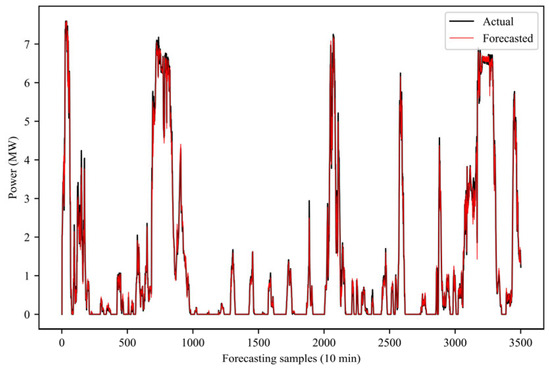
Figure 10.
Power forecasting in all periods.
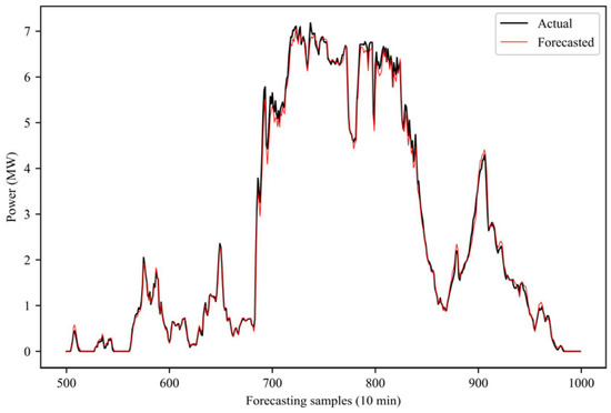
Figure 11.
Power forecasting for some periods.
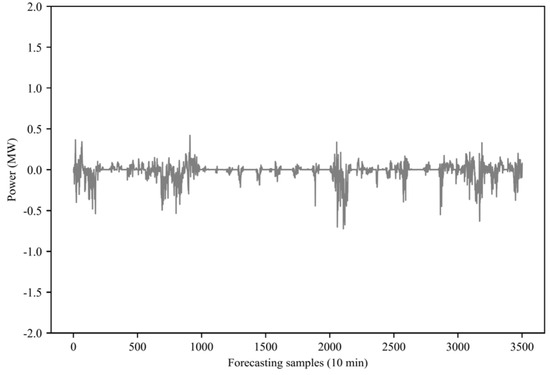
Figure 12.
Power forecasting error in all periods.
4.3.1. Comparison with Mainstream Methods
In this section, the proposed method is compared with other advanced forecasting models, including CNNs, RNNs, LSTM, GRU, and hybrid neural networks.
The output results of the comparison model are shown in Figure 13 and Figure 14. In the sequence model, in terms of the MAE index, RNN has the best performance, followed by GRU, and LSTM has the worst performance. The higher the complexity of this type of network, the lower the forecasting accuracy, and even CNN has achieved similar results as RNN. This is because the data used are collected from a single wind turbine, and the physical attribute data of wind power are highly correlated with the forecasted power, which is higher than the historical power change trend.
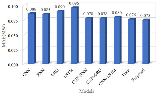
Figure 13.
A histogram of an MAE performance comparison for different models.
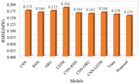
Figure 14.
RMSE performance comparison histogram for different models.
In addition, although the MAE index of CNN achieved similar results to those of RNN, even lower than those of GRU, its RMSE is higher than that of RNN and GRU, indicating that CNN has the problem of insufficient forecasting stability, while RNN, LSTM, and GRU have the problem of insufficient forecasting accuracy. Therefore, many researchers combine CNN with RNN, LSTM, and GRU to form a hybrid neural network to make up for the deficiency. The results show that the hybrid neural network can effectively improve the forecasting accuracy and stability of the model.
Although the hybrid neural network was able to achieve higher forecasting accuracy, the accuracy is slightly lower than that of the Transformer model. The reason is that the Transformer model can effectively capture long-distance dependence and ignore the limitation of spatial distance.
However, the model proposed in this paper shows stronger performance. The main reasons can be attributed to the following two points:
- (1)
- Stacked multi-layer perceptron has strong nonlinear expression ability. The model can gradually extract high-level features of the data, which is more suitable for scenarios such as wind power forecasting that require high nonlinearity.
- (2)
- Multi-view extraction of data features with different attributes can avoid homogenization extraction and enrich the feature expression that affects future power. The relationship between future power and input data is effectively established.
Compared with other models, the MAE index of the proposed method is reduced by 21.88% at most, and the RMSE is reduced by 16.85% at most.
4.3.2. Sensitivity Analysis
In this section, the performance of the proposed model is compared with other models in more detail through sensitivity analysis. As shown in Table 2 and Table 3, the MAE and RMSE of multiple running results are shown. In MAE and RMSE, the proposed model shows the lowest error in Best, Median, Mean, and Worst. It is worth noting that the Worst (i.e., the highest error of multiple runs) of the model proposed in this paper is close to the Best value of other models, although its std is slightly higher than some models. It can be concluded that the wind power forecasting performance of the proposed model is significantly better than other advanced models.
Table 2.
Comparison results of forecasting models on MAE.
Table 3.
Comparison results of forecasting models on RMSE.
4.3.3. Rolling Forecasting
In this section, the rolling forecasting of the proposed model is introduced to verify the advanced multi-step forecasting performance of the model. It should be noted that the structure and parameters of all models remain unchanged, and the step size of the rolling forecasting is 6, that is, the wind power of 1h is forecasted in advance (the data sampling interval is 10 min). The forecasting results of the forecasting model are shown in Table 4. It can be observed that the proposed model achieved an absolute advantage over other models, with a minimum reduction of 12.50% and 14.67% in MAE and RMSE, and a maximum reduction of 31.58% and 40.92%.
Table 4.
Rolling forecasting error of forecasting model.
Compared with single-step forecasting, the advantages of the proposed model in multi-step forecasting scenarios are more obvious. The reason is that the multi-step forecasting demand model has stronger nonlinear reasoning ability. The nonlinear reasoning ability of other models is obviously insufficient, so the forecasting accuracy is lower than that of the model proposed in this paper.
In addition, it also shows the rolling forecasting results of the forecasting model for the whole period of time, as shown in Figure 15, the partial period forecasting results, as shown in Figure 16, and the partial period forecasting error, as shown in Figure 17. It can be observed that there is a large deviation between the forecasted power and the actual power during the continuous power peak period. From some forecasting results and forecasting errors, it can be seen that the forecasting volatility of the model proposed in this paper is the smallest in this region, and the forecasting results are closer to the real power value.
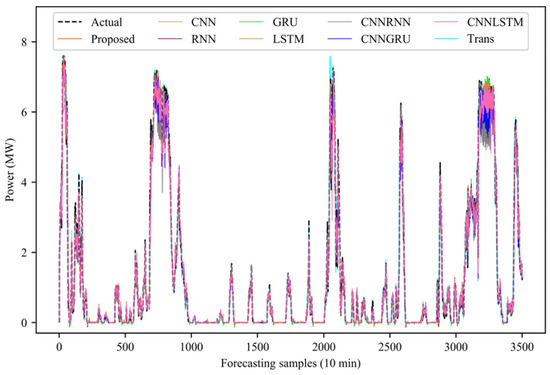
Figure 15.
Full-time model rolling forecasting.
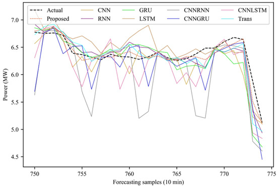
Figure 16.
Partial period model rolling forecasting.
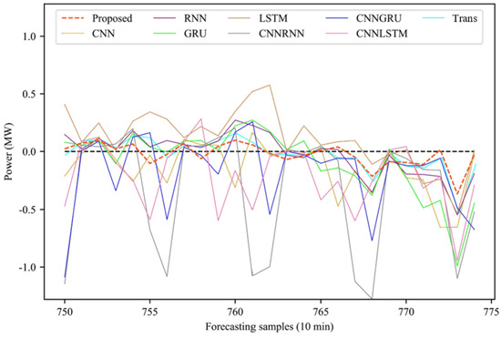
Figure 17.
Rolling forecasting error of partial time period model.
5. Case Study 2
This paper sets up Case Study 2 to prove the generalization performance of the proposed model. The wind power data used in this case were collected from Ningxia Province, China. The total installed capacity of the wind farm is 100 MW, and the data sampling resolution is 15 min. The input data can be provided as shown in Table 5.
Table 5.
Forecasting error of forecasting model on Case 2.
In order to reflect the generalization performance of the model, the parameters set by the model are the same as those in Case Study 1. The forecasting results under three forecasting steps are shown in Table 6.
Table 6.
Data list of Case 2.
The research scenario of this case is a centralized wind farm. Due to the power cumulative effect [22], the power fluctuation of the centralized wind farm is lower than that of the distributed wind farm in Case 1. Therefore, the nonlinear requirement of the model is low. Therefore, the performance advantage of the model proposed in this paper is not obvious. Compared with the Transformer model, MAE and RMSE are only reduced by 0.98% and 0.92%, respectively, in the 45 min forecasting scenario. Although the advantages are not obvious, the proposed model has the best forecasting accuracy in both distributed wind farms and centralized wind farms. The results prove the generalization ability of the model from the side.
6. Conclusions
Wind power generation has strong nonlinearity, resulting in insufficient forecasting accuracy. In this paper, a pseudo-twin neural network based on full multi-layer perceptron is proposed for wind power forecasting. Based on the multi-layer perceptron, the model improves the extraction and fusion ability of relevant forecasting features by constructing MLP-E and MLP-M modules, and uses a multi-view feature fusion strategy to provide complementary information.
Using actual operational data from wind turbines or wind farms, this paper conducts a comparative analysis between the proposed model and other models. The results from two case studies demonstrate that, compared to the CNN model in reference [11], the proposed model reduces the forecasting MAE by an average of 15.36%. When compared to the sequence models in references [12,13,14], the forecasting MAE is reduced by an average of 12.97%. Additionally, compared to the hybrid neural networks in references [12,15], the forecasting MAE is reduced by an average of 9.38%. These results indicate that the proposed model can effectively improve the accuracy of ultra-short-term wind power forecasting, providing a robust reference for power scheduling on wind farms.
However, the proposed model still has limitations. In particular, there are too many limitations in the model parameters. Model parameters are difficult to update in real time to adapt to new forecasting scenarios. In the following research, model pruning, compression, and other technologies will be used to reduce the model parameters and improve the training efficiency while maintaining the forecasting accuracy.
Author Contributions
Y.Y.: Resources and Writing—review and editing; J.W.: Methodology, Software, and Writing—original draft; B.C.: Investigation and Supervision; H.Y.: Software. All authors have read and agreed to the published version of the manuscript.
Funding
This research was funded by the following project: key technologies for flexible interactive flexible control of multi-load and new energy (2022B01020-4).
Data Availability Statement
Relevant data have been shared in the paper.
Conflicts of Interest
All authors declare that the research was conducted in the absence of any commercial or financial relationships that could be construed as a potential conflict of interest.
References
- Fan, H.; Zhen, Z.; Liu, N.; Sun, Y.; Chang, X.; Li, Y.; Wang, F.; Mi, Z. Fluctuation pattern recognition based ultra-short-term wind power probabilistic forecasting method. Energy 2023, 266, 126420. [Google Scholar] [CrossRef]
- Liu, Z.; Guo, H.; Zhang, Y.; Zuo, Z. A Comprehensive Review of Wind Power Prediction Based on Machine Learning: Models, Applications, and Challenges. Energies 2025, 18, 350. [Google Scholar] [CrossRef]
- Xu, Z.-Q.; Xue, T.; Chen, X.-Y.; Feng, J.; Zhang, G.-W.; Wang, C.; Lu, C.-H.; Chen, H.-S.; Ding, Y.-H. Wind power correction model designed by the quantitative assessment for the impacts of forecasted wind speed error. Adv. Clim. Change Res. 2024. [Google Scholar] [CrossRef]
- Cunha, J.L.; Pereira, C.M. A hybrid model based on STL with simple exponential smoothing and ARMA for wind forecast in a Brazilian nuclear power plant site. Nucl. Eng. Des. 2024, 421, 113026. [Google Scholar] [CrossRef]
- Taylor, J.W. Probabilistic forecasting of wind power ramp events using autoregressive logit models. Eur. J. Oper. Res. 2017, 259, 703–712. [Google Scholar] [CrossRef]
- Chen, Y.; Xiao, J.-W.; Wang, Y.-W.; Luo, Y. Non-crossing quantile probabilistic forecasting of cluster wind power considering spatio-temporal correlation. Appl. Energy 2025, 377, 124356. [Google Scholar] [CrossRef]
- Khan, S.; Muhammad, Y.; Jadoon, I.; Awan, S.E.; Raja, M.A.Z. Leveraging LSTM-SMI and ARIMA architecture for robust wind power plant forecasting. Appl. Soft Comput. 2025, 170, 112765. [Google Scholar] [CrossRef]
- Liu, X.; Lin, Z.; Feng, Z. Short-term offshore wind speed forecast by seasonal ARIMA-A comparison against GRU and LSTM. Energy 2021, 227, 120492. [Google Scholar] [CrossRef]
- Huang, B.; Liang, Y.; Qiu, X. Wind power forecasting using attention-based recurrent neural networks: A comparative study. IEEE Access 2021, 9, 40432–40444. [Google Scholar] [CrossRef]
- Zhang, G.; Zhang, L.; Xie, T. Prediction of Short-Term Wind Power in Wind Power Plant Based on BP-ANN. In Proceedings of the 2016 IEEE Advanced Information Management, Communicates, Electronic and Automation Control Conference (IMCEC), Xi’an, China, 3–5 October 2016; pp. 75–79. [Google Scholar]
- Chen, G.; Shan, J.; Li, D.Y.; Wang, C.; Li, C.; Zhou, Z.; Wang, X.; Li, Z.; Hao, J.J. Research on Wind Power Prediction Method Based on Convolutional Neural Network and Genetic Algorithm. In Proceedings of the 2019 IEEE Innovative Smart Grid Technologies-Asia (ISGT Asia), Chengdu, China, 21–24 May 2019; pp. 3573–3578. [Google Scholar]
- Zhao, Z.; Yun, S.; Jia, L.; Guo, J.; Meng, Y.; He, N.; Li, X.; Shi, J.; Yang, L. Hybrid VMD-CNN-GRU-based model for short-term forecasting of wind power considering spatio-temporal features. Eng. Appl. Artif. Intell. 2023, 121, 105982. [Google Scholar] [CrossRef]
- Al-Qaness, M.A.; Ewees, A.A.; Aseeri, A.O.; Elaziz, M.A. Wind power forecasting using optimized LSTM by attraction–repulsion optimization algorithm. Ain Shams Eng. J. 2024, 15, 103150. [Google Scholar] [CrossRef]
- Kisvari, A.; Lin, Z.; Liu, X. Wind power forecasting–A data-driven method along with gated recurrent neural network. Renew. Energy 2021, 163, 1895–1909. [Google Scholar] [CrossRef]
- Houran, M.A.; Bukhari, S.M.S.; Zafar, M.H.; Mansoor, M.; Chen, W. COA-CNN-LSTM: Coati optimization algorithm-based hybrid deep learning model for PV/wind power forecasting in smart grid applications. Appl. Energy 2023, 349, 121638. [Google Scholar] [CrossRef]
- Goutte, S.; Klotzner, K.; Le, H.-V.; von Mettenheim, H.-J. Forecasting photovoltaic production with neural networks and weather features. Energy Econ. 2024, 139, 107884. [Google Scholar] [CrossRef]
- Jiang, H.; Liu, D.; Ding, X.; Chen, Y.; Li, H. TCM: An efficient lightweight MLP-based network with affine transformation for long-term time series forecasting. Neurocomputing 2025, 617, 128960. [Google Scholar] [CrossRef]
- Wang, Y.; Zhou, X. Predictive study of drying process for limonite pellets using MLP artificial neural network model. Powder Technol. 2024, 444, 120026. [Google Scholar] [CrossRef]
- Zhang, R.; Wu, Y.; Zhang, L.; Xu, C.; Wang, Z.; Zhang, Y.; Sun, X.; Zuo, X.; Wu, Y.; Chen, Q. A multiscale network with mixed features and extended regional weather forecasts for predicting short-term photovoltaic power. Energy 2025, 318, 134792. [Google Scholar] [CrossRef]
- Liu, H.; Yan, S.; Huang, M.; Huang, Z. A fault diagnosis method for hydraulic system based on multi-branch neural networks. Eng. Appl. Artif. Intell. 2024, 137, 109188. [Google Scholar] [CrossRef]
- Tolstikhin, I.O.; Houlsby, N.; Kolesnikov, A.; Beyer, L.; Zhai, X.; Unterthiner, T.; Yung, J.; Steiner, A.; Keysers, D.; Uszkoreit, J. Mlp-Mixer: An all-mlp architecture for vision. Adv. Neural Inf. Process. Syst. 2021, 34, 24261–24272. [Google Scholar]
- Mu, G.; Wu, F.; Zhang, X.; Fu, Z.; Xiao, B. Analytic mechanism for the cumulative effect of wind power fluctuations from single wind farm to wind farm cluster. CSEE J. Power Energy Syst. 2022, 8, 1290–1301. [Google Scholar]
Disclaimer/Publisher’s Note: The statements, opinions and data contained in all publications are solely those of the individual author(s) and contributor(s) and not of MDPI and/or the editor(s). MDPI and/or the editor(s) disclaim responsibility for any injury to people or property resulting from any ideas, methods, instructions or products referred to in the content. |
© 2025 by the authors. Licensee MDPI, Basel, Switzerland. This article is an open access article distributed under the terms and conditions of the Creative Commons Attribution (CC BY) license (https://creativecommons.org/licenses/by/4.0/).