Multi-Factor Task Assignment and Adaptive Window Enhanced Conflict-Based Search: Multi-Agent Task Assignment and Path Planning for a Smart Factory

Abstract

Multi-Agent Systems (MAS) are widely deployed in smart factory environments, where efficient task assignment and path planning for agents can greatly enhance production efficiency. Existing algorithms usually ignore resource constraints, overly simplify the geometric shape of agents, and perform poorly in large-scale scenarios. In this paper, we propose a Multi-Factor Task Assignment and Adaptive Window Enhanced Conflict-Based Search (MTA-AWECBS) algorithm to solve these problems, which considers the resource constraints and volume of agents, improving the algorithm’s scalability and adaptability. In task assignment, a novel scheme is designed by considering distance cost, maximum travel distances, and maximum number of executable tasks. In path planning, we first propose a new mathematical description of global traffic congestion level. Based on this, an adaptive window is proposed to dynamically adjust the time horizon in the WECBS algorithm, improving search efficiency and solving the deadlock issue. Additionally, based on experimental observations, two optimization strategies are proposed to further improve operation efficiency. The experimental results show that MTA-AWECBS outperforms Token Passing (TP), Token Passing with Task Swaps (TPTSs), and Conflict-Based Steiner Search (CBSS) in handling a large number of tasks and agents, achieving an average $39\%$ reduction in timestep cost and an average $22\%$ reduction in total path cost.

1. Introduction

Smart factories, as a key part of Industry 4.0, need to achieve high operational efficiency and low costs of production [1]. Numerous innovative manufacturing schemes have already been proposed to meet these needs. Among these schemes, the multi-agent system (MAS) is one of the most representative due to its flexibility and efficiency [2,3]. There are two key problems that need to be solved in the MAS. One is the multi-agent task assignment (MATA) problem [4], which assigns suitable tasks to each agent to ensure that tasks are completed quickly and efficiently. The other is the multi-agent path planning (MAPF) problem [5], which aims to find a conflict-free path for each agent from its starting location to its destination. Conflict-free means that agents will not collide with other agents while traveling along their path. Multi-agent task assignment and path planning (TAPF) [6], a hot research topic that combines MATA and MAPF, requires solving both task assignment and path planning. Solving each problem individually may consume a lot of time, so it is important to solve both problems together and obtain a good solution within the limited time available. TAPF plays a crucial role in Industry 4.0, particularly in raw material delivery [7], parts delivery [8], and production line status monitoring [9]. An appropriate solution can greatly improve operational efficiency and reduce costs, meeting the requirements of Industry 4.0 for high efficiency.

Although the TAPF problem has been widely investigated by many scholars, naively applying existing methods to real-world smart factories is not a wise choice for the following reasons. Firstly, real-world restrictions must be considered in productive environments. For example, the limited battery capacity, complex geometric shape, and task execution capabilities of agents. These factors are often oversimplified in previous methods. The famous Conflict-Based Search with Task Assignment (CBS-TA) algorithm proposed by Hönig et al. [10] can find an optimal solution for the TAPF problem, but it only considers the distance cost and overlooks the factors discussed above. Tang et al. [11] extended the CBS-TA and developed a new optimal algorithm called Incremental Target Assignment-Conflict-Based Search (ITA-CBS), which resolves the issue of duplicated conflicts to reduce computational complexity and improve search efficiency. Unfortunately, ITA-CBS still only considers distance factors and thus does not fully capture important aspects of real factory applications. Chen et.al. [12] considered agent capacity limitations, and Kudo et al. [13] focused on the maximum load and delivery cost. However, both of these methods fail to further consider important factors such as the agents’ battery resources, actual volume, and execution capabilities. All these methods hardly provide effective support for real productive scenarios.

Secondly, most research focuses on finding a conflict-free path for each agent, ignoring the overall congestion level, which directly impacts throughout, leading to low production efficiency in real-world factories. Li et al. [14] proposed the windowed ECBS algorithm for lifelong path planning and improved throughput. However, the time horizon in this method is fixed and fails to provide a quantitative description of the congestion level in the scenario, which may result in the occurrence of deadlocks in highly congested scenarios. Song et al. [15] proposed a novel lifelong MAPF method, which further enhances throughput and reflects traffic congestion through delay time. However, it still lacks a mathematical model for quantitatively describing the global congestion level. Chen et al. [16] proposed a congestion-aware routing method that plans paths to avoid congested areas and effectively handles dynamic traffic conditions. However, the scalability of this approach remains somewhat limited. Optimizing the TAPF algorithm is crucial for enhancing throughput and preventing deadlock occurrences. Such improvements require a precise metric that objectively reflects the overall congestion level.

Finally, yet importantly, most existing algorithms suffer poor scalability, and timeout failures are likely to happen when handling large-scale factory scenarios. For example, although the CBS-TA method [10] guarantees solution quality, it only produces satisfactory results on small-scale problem sets. Henkel et al. [17] proposed an optimal solution for TAPF where each agent can execute more than one task, but it scales to only four agents and four tasks. In addition, some researchers have already noticed the link between TAPF and the Traveling Salesman Problem (TSP) and have developed solutions based on this observation, yet these methods still face the challenge of addressing NP-hard problems TSP [18,19,20]. Therefore, their main issue is that the success rate of algorithms is low because timeout failures often happen when the number of agents and tasks becomes relatively large.

These drawbacks limit practical deployments in real smart factories where the multi-agent system scale is often large, with real-world additional constraints, and deadlocks are never allowed. Our work aims to overcome these shortcomings. Before diving into the details, we summarize our contribution as follows:

(1) A new mathematical description of global traffic congestion level is proposed for multi-agent systems, along with a corresponding analysis of its validity. Based on this, an adaptive windowed ECBS algorithm is proposed to dynamically adjust the time horizon during path planning, effectively resolving traffic jams and completely avoiding deadlock issues. The algorithm reduces the average congestion level by $31\%$ in a real factory environment.

(2) There are two situations that are often ignored in many studies and frequently occur in the TAPF problem. To address this, we propose two corresponding optimization strategies that intervene at specific time steps, providing a finer-grained task assignment schedule and exploring a broader solution space. These strategies further enhance the algorithm’s performance and adaptability in complex factory environments, resulting in a $24\%$ reduction in average timestep cost and a $13\%$ reduction in total path cost.

(3) Building upon the above, we further expand conventional TAPF research by considering necessary constraints in real factory environments, such as agents’ resource limitations, including maximum travel distance and maximum number of executable tasks. Additionally, agents are no longer regarded as points for path planning; instead, their actual volume is taken into account.

The rest of this paper is organized as follows: Section 2 introduces relevant approaches and algorithms for TAPF. Section 3 formally defines the TAPF problem and related notations. Section 4 describes the proposed MTA-AWECBS algorithm. Section 5 provides a detailed experimental comparison of MTA-AWECBS with other TAPF algorithms. Section 7 concludes the paper and summarizes its content.

2. Related Work

The multi-agent task assignment (MATA) problem is a crucial component of TAPF, which requires assigning suitable tasks to each agent. Various approaches have been proposed to solve this problem. A classic and well-known algorithm is the Hungarian algorithm [21], which is adopted by Honig in their work to obtain the task assignment scheme [10]. Xu et al. [22] modified the Hungarian algorithm by introducing a Large Neighborhood Search Strategy (LNS) [23] to improve the assignment scheme. Additionally, heuristic-based approaches [12,24,25,26] and auction-based approaches [27] have been widely used because of their effectiveness in solving task assignment problems across many scenarios. Bai et al. [24] used a simulated annealing algorithm to solve the task assignment problem and applied local search approaches to improve the solution. Bai et al. [27] designed two group-based distributed auction algorithms to solve the task assignment problem, enabling the robots to independently choose feasible package groups that they can serve. In recent years, some researchers [18,19,20] have created a link between MATA and the TSP, regarding the multi-agent task assignment problem as a Traveling Salesman Problem [28]. However, most of the aforementioned research on task assignment considers only a single factor. For example, references [10,12,18,19,20,24] mainly focus on distance factors.

The multi-agent path finding (MAPF) problem is another important part of TAPF, which aims to plan conflict-free paths for each agent from their respective starts to their destinations [5]. Existing approaches to solving the MAPF problems can be categorized as optimal algorithms, suboptimal algorithms, priority-based algorithms, and rule-based algorithms. Conflict-Based Search (CBS) [29] as a typical optimal MAPF algorithm is widely used. It is composed of a high-level and a low-level layer, where the high level is responsible for finding conflicts between paths, resolving these conflicts, and adding constraints, while the low level replans each agent’s path based on the constraints provided by the high level. It is famous for its extensibility and has many variant algorithms [30,31]. CBS and its variations provide optimal solutions, but they suffer from poor scalability and slow search speed. To overcome their weakness, suboptimal algorithms such as Enhanced Conflict-Based Search (ECBS) [32] have emerged, which sacrifice the optimal solution in exchange for faster search speed. Li et al. [33] proposed the Explicit Estimation CBS (EECBS) algorithm, which utilizes explicit estimation search and three heuristic functions, further enhancing performance. These suboptimal algorithms compromise the optimal solution for greater algorithm scalability and faster search speed, making them suitable for scenarios where efficiency is crucial, such as in smart factories where problems must be solved within a limited time. In this paper, we adopt the suboptimal algorithm ECBS for path planning and provide a detailed explanation in the path planning section. Priority-based algorithms, like the Priority-Based Search (PBS) algorithm [34], plan paths by assigning priority orders to agents. But priority-based algorithms lack robustness and may not deliver satisfactory solutions in complex scenarios. Rule-based algorithms plan paths based on certain rules. Push and Swap [35] resolves conflicts with pre-defined rules and guarantees finding a solution to the MAPF problem in polynomial time; however, the quality of these solutions is far from optimal. These MAPF algorithms mentioned above are generally designed for scenarios where the number of agents equals the number of tasks, limiting their application in smart factories because the number of agents and tasks within the factory can be in any proportion.

The TAPF problem is a combination of the MATA problem and the MAPF problem [6]. Different methods have been proposed to solve the complex problem. For instance, H. Ma et al. [36] proposed Token Passing (TP) and Token Passing with Task Swaps (TPTSs) algorithms to tackle TAPF problems in automated warehouses scenarios. These algorithms can handle problems with hundreds of agents and tasks but at the cost of lower solution quality. Fang et al. [37] developed a task and path planning method for a factory environment. In addition to the aforementioned scenarios, Li et al. [38] proposed a task and path planning algorithm for the circuit inspection scenario, incorporating the effect of wind fields in task assignment. Huo et al. [39] developed a multi-stage optimization method for Automated Guided Vehicle (AGV) cargo transportation scenarios, effectively facilitating cargo transportation with multiple AGVs. Additionally, other advanced methods, such as the MS* [18] algorithm, treat task assignment as the Traveling Salesman Problem and use a heuristic policy to generate a task assignment sequence for each agent. For path planning, they employ an improved algorithm based on the M* [40] algorithm. Unfortunately, the scalability of the algorithm is weak, and the success rate of the algorithm decreases as the number of agents exceeds 10. Ren et al. [19] developed the Conflict-Based Steiner Search (CBSS) algorithm, which achieves higher success rates than MS*, but its scalability is still limited, and the success rate of the algorithm is relatively low when the number of agents exceeds 50. Nguyen et al. [41] innovatively used answer set programming to solve the TAPF problem and achieve an exact solution. However, the approach is only scalable to 20 agents, each executing approximately four tasks. Besides these approaches, there are also many other TAPF solution methods, such as how Okumura et al. [42] proposed the TSWAP and Shimizu et al. [43] proposed an algorithm for TAPF problems for AGV kinematics. These TAPF algorithms mostly have several common problems. Firstly, they primarily focus on distance factors in TAPF. Secondly, these algorithms cannot be applied to large-scale scenarios like real factories due to poor scalability. Furthermore, the modeling of agents is usually oversimplified in these algorithms, treating them merely as points, but smart robots usually occupy space that is hardly ignorable in smart factories because the geometric shape of agents directly impacts operational efficiency. So, treating agents as points is inappropriate.

3. Problem Definition

The TAPF problem is usually modeled as follows. Let $G=(V,E)$ be an undirected connected graph, where $V=\{{\mathit{v}}_1,{\mathit{v}}_2,\dots ,{\mathit{v}}_n\}$ is a set of vertices, representing the possible locations for agents; $E=\{e_1,e_2,\dots ,e_m\}$ is the set of edges connecting two different vertices, indicating a passage between those locations. Each edge $e\in E$ has a unit length, and self-loop edges are allowed, which correspond to “wait-in-current-location” actions. Let $A=\{a_1,a_2,\dots ,a_k\}$ be the set of k agents, and each agent $a_i$ has a respective starting position $s_i\in V$. Let ${\mathit{v}}_i\left(t\right)\in V$ denote the location of $a_i$ at discrete timestep t. In each timestep t, an agent $a_i$ can choose either to wait in its current location ${\mathit{v}}_i\left(t\right)$ or move along an edge to an adjacent location. Both waiting and moving consume one timestep cost. Let $M=\{m_1,m_2,\dots ,m_s\}$ be the set of s tasks, with no priority among them. Each agent $a_i$ can be assigned a task $m_j$ from M. In our model, an individual agent $a_i$ can have multiple tasks, and each task has a designated location. We use a set $\mathcal{M}=\left\{g\right(1),g(2),\dots ,g(s\left)\right\}$ to denote the actual positions corresponding to the s tasks in the task set M.

A path $P_i=\langle {\mathit{v}}_i\left(0\right),{\mathit{v}}_i\left(1\right),{\mathit{v}}_i\left(2\right),\dots ,{\mathit{v}}_i\left(t\right)\rangle$ denotes the sequence of vertices traversed by the agent $a_i$ from starting point to target point. The agent $a_i$ starts its movement from the initial position, i.e., ${\mathit{v}}_i\left(0\right)=s\left(i\right)$, and reaches its assigned target position, i.e., ${\mathit{v}}_i\left(t\right)=g\left(i\right)\in \mathcal{M}$. Define $\mathit{P}=\{P_1,P_2,\dots ,P_k\}$ to be the set of all agent paths. A solution $\mathcal{P}$ to the TAPF problem is a conflict-free $\mathit{P}$ minimizing the cost of paths.

To minimize path costs, numerous existing criteria can be used, among which the most widely used are Makespan (ms) and Sum of costs (soc) [5]. ms is the number of timesteps required for all agents to reach their target, i.e., the timestep cost. soc is the sum of timesteps required for each agent to reach its target, i.e., the total path cost. This paper adopts the soc as the optimization criterion.

In addition to minimizing path costs, a solution $\mathcal{P}$ must not have conflicts. Classic conflict can mainly be categorized as vertex conflict and edge conflict, as shown in Figure 1a and Figure 1b.

(1) Vertex Conflict: A vertex conflict is commonly characterized by a four-element tuple $\langle a_i,a_j,\mathit{v},t\rangle$ where ${\mathit{v}}_i\left(t\right)={\mathit{v}}_j\left(t\right)\in V$. Such a tuple indicates that agent $a_i$ and $a_j$ are at the same position at the same timestep, as shown in Figure 1a.

(2) Edge Conflict: An edge conflict can be described by a five-element tuple $\langle a_i,a_j,{\mathit{v}}_1,{\mathit{v}}_2,t\rangle$ where ${\mathit{v}}_i(t+1)={\mathit{v}}_j\left(t\right)$ and ${\mathit{v}}_j(t+1)={\mathit{v}}_i\left(t\right)$ meaning that agent $a_i$ and $a_j$ cross each other in the timestep after t, as shown in Figure 1b.

Besides the classic model formulation, some constraints have to be considered in TAPF problems that arise in real factories and are crucial for production, so a detailed explanation will be provided in the following.

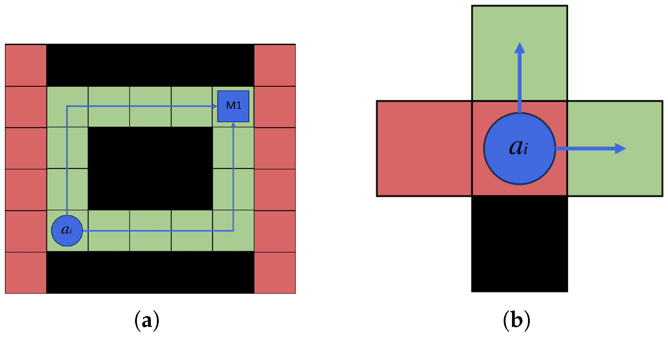
3.1. Maximum Travel Distance

The travel distance of each real agent has an upper limit because they are constrained by battery capacity and signal range. Although the maximum travel distance may vary among different agents, we assume in this paper that all agents have the same maximum travel distance. The constraint requires agents to return for recharging and prevents them from traveling beyond the factory’s signal range. The maximum travel distance is denoted by $D_{max}$, meaning the maximum travel distance for agent $a_i$ is less than or equal to $D_{max}$.

3.2. Maximum Number of Executable Tasks

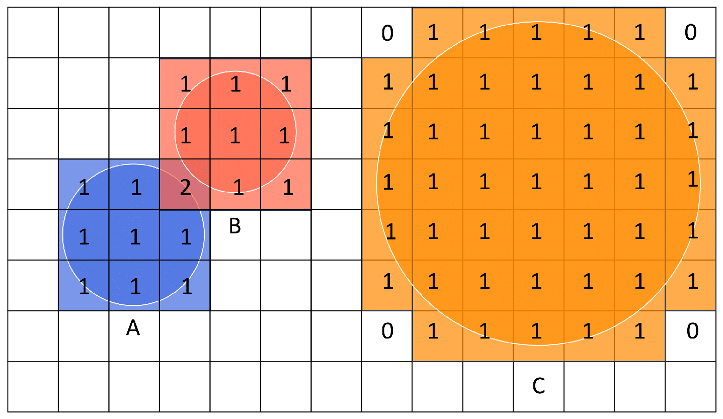
The task execution capacity of each agent is limited, and overloading may lead to performance degradation. Therefore, task load balancing is essential for agents in a factory environment. Although various approaches can be employed to implement load balancing, setting a maximum number of executable tasks is a simple and effective approach. We assume that all agents have the same maximum number of executable tasks, ignoring any agent heterogeneity. The maximum number of executable tasks is denoted by $N_{max}$, meaning the number of tasks that agent $a_i$ can execute is less than or equal to $N_{max}$.

3.3. Agent Geometry

In this paper, each agent is no longer regarded as a point, and its actual volume is taken into account. Thus, the previous conflict representation methods are no longer suitable. As shown in Figure 2, two agent vehicles (red and blue) have not reached vertex $\mathit{v}$, but a conflict has already occurred due to their volume sizes. In real factory settings, agents cannot be simplified as points, therefore, our algorithm must be updated to handle volume collisions as shown in Figure 2.

We made a simple modification to the classic approach by modeling agents of different sizes using their circumcircles. As shown in Figure 3, agents A (blue) and B (red) occupy multiple grids, with $r_a=2.5$ and $r_b=1.5$ denoting the radius of their respective circumcircles. Although this modeling is very rough, it is enough to avoid collisions shown in Figure 2. To represent the space occupied by agents in the grid map, any grid cell that the circumcircle overlaps is considered to be occupied by the agent. For example, the space occupied by agent A is a 5 × 5 rectangular area, while agent B occupies a 3 × 3 rectangular area. We use the center grid to represent the current position of the agent. Therefore, the position of A is (4, 6), and the position of B is (6, 3). Although agents A and B are in different locations, a conflict still occurs.

Consequently, the conflict model must now be refined under this new characterization of agents. The vertex conflict is refined as a five-element tuple $\langle a_i,a_j,{\mathit{v}}_i,{\mathit{v}}_j,t\rangle$, where ${\mathit{v}}_i$ represents the position of agent $a_i$ at timestep t, and ${\mathit{v}}_j$ represents the position of agent $a_j$ at timestep t. This tuple indicates at the same timestep t, agent $a_i$ at vertex ${\mathit{v}}_i$ conflicts with agent $a_j$ at vertex ${\mathit{v}}_j$. The edge conflict is refined as a seven-element tuple $\langle a_i,a_j,{\mathit{v}}_i,{\mathit{v}}_j,{\mathit{v}}_i^{\prime },{\mathit{v}}_j^{\prime },t\rangle$, meaning that at the same timestep t, agent $a_i$ moving from vertex ${\mathit{v}}_i$ to vertex ${\mathit{v}}_j$ conflicts with another agent $a_j$ moving from vertex ${\mathit{v}}_i^{\prime }$ to vertex ${\mathit{v}}_j^{\prime }$. A special case is that when the radius r of the circumcircle of the agent is greater than 0.5, edge conflict will never happen because we are dealing with integer grid spaces and using a four-connected grid map in this paper.

These additional constraints are crucial for real smart factory production. The maximum travel distance, the maximum number of executable tasks, and the volume of agents make the TAPF problem more suited for smart factory environments. Based on these considerations, we propose the TAPF solution: the Multi-Factor Task Assignment and Adaptive Window Enhanced Conflict-Based Search (MTA-AWECBS) algorithm.

4. TAPF Solution

The MTA-AWECBS algorithm, like other contemporary algorithms [23,24,25], is divided into two parts: task assignment and path planning. In task assignment, an appropriate task scheme is assigned to each agent. In path planning, a conflict-free path is generated for each agent according to its assigned tasks.

4.1. Task Assignment

In the task assignment, a reasonable task assignment model is designed considering distance cost, maximum travel distances, and maximum number of executable tasks. Subsequently, we propose the Multi-Factor Hungarian Assignment Algorithm to solve the task assignment scheme.

4.1.1. MATA Problem Modeling

In the MATA problem, each task needs to be assigned to an agent and each agent can only execute one task at a time. Once the agent completes its current task, it will immediately be reassigned a new task. If an agent has not been assigned any tasks, it is referred to as an idle agent. Therefore, an agent that has just completed a given task is also an idle agent. Let $x_{ij}$ equal 1 if agent $a_i$ executes task $m_j$, and 0 otherwise.

$$x_{ij}=\left\{\begin{array}{cc}\hfill 1& \mathrm{if}{a}_i\mathrm{executes}\mathrm{tasks}{m}_j\hfill \\ \hfill 0& \mathrm{otherwise}\hfill \end{array}\right.$$

(1)

Let $C={\left(c_{ij}\right)}_{m\times n}$ denote the cost matrix, which is a map attribute used to describe the distance costs between vertices in the map. Let $\mathit{c}:V\times V\mapsto {\mathbb{Z}}_{+}\ge 0$ be a function that maps from the product of $V\times V$ to a distance cost value. The element $c_{ij}$ is calculated using the function $\mathit{c}({\mathit{v}}_i,{\mathit{v}}_j)$, which means the distance cost from ${\mathit{v}}_i$ to ${\mathit{v}}_j$ avoiding all the obstacles. For the $\mathit{c}({\mathit{v}}_i,{\mathit{v}}_j)$, unlike previous approaches that estimated distances using either Euclidean or Manhattan, we use actual shortest distances obtained through the BFS algorithm [44] and cache them appropriately, avoiding the time spent on repeated calculations in the future. As shown in the Section 3, there is a set A containing k agents and a set M containing s tasks. Thus, the MATA problem can be described as

$$\mathrm{minimize}\sum _{i=1}^k\sum _{j=1}^s{c}_{ij}{x}_{ij}$$

(2)

where

$$\sum _{i=1}^k{x}_{ij}=11\le j\le s$$

(3)

The constraint Equation (3) ensures that every task is assigned to a specific agent. Most MATA studies only consider the distance factor and include only Equation (3). However, in this paper, additional constraints are introduced:

$$\sum _{j=1}^s{c}_{ij}{x}_{ij}\le D_{max}1\le i\le k$$

(4)

$$\sum _{j=1}^s{x}_{ij}\le N_{max}1\le i\le k$$

(5)

The constraint Equation (4) corresponds to the maximum travel distance $D_{max}$, which guarantees that the travel distance of each agent does not exceed the $D_{max}$, avoiding battery energy depletion and restricting their work range. Constraint Equation (5) corresponds to the maximum number of executable tasks $N_{max}$, which ensures that the number of tasks assigned to each agent does not exceed the $N_{max}$, keeping work efficiency.

4.1.2. Multi-Factor Hungarian Assignment Algorithm

This paper aims to solve the TAPF problem in large-scale scenarios, with the ultimate objective of planning collision-free paths for agents. The task assignment should be time-efficient and able to handle a large number of tasks. The Hungarian algorithm [21] is the optimal choice due to its key advantage of fast solution speed. Unlike other heuristic algorithms that require complex iterative procedures, this method solves the problem through matrix transformations in polynomial time, thus achieving faster results. Directly applying it to solve the MATA problem in a smart factory presents some challenges, such as how to introduce constraint conditions $D_{max}$ and $N_{max}$, and how to solve mismatches between the number of agents and tasks.

The first challenge is how to integrate the constraints $D_{max}$ and $N_{max}$ into the Hungarian algorithm. In each task assignment, the Hungarian algorithm only assigns one task to each agent. Before formally constructing the task cost matrix, we will select agents that meet the two constraint conditions for task assignment. Another challenge is that the Hungarian algorithm requires a square cost matrix, $m=n$, meaning the number of agents must be equal to the number of tasks. However, this paper aims to solve the problem of large-scale TAPF in a smart factory environment, where the number of agents and tasks can be in any proportion. To handle this problem, various modifications and extensions of the Hungarian algorithm have been developed [45]. We follow these approaches by setting virtual agents (or tasks) to balance the number of tasks and agents. Virtual agents do not really execute any tasks and disappear in the next assignment.

After solving the above challenges, we propose an improved Hungarian algorithm called the Multi-Factor Hungarian Assignment algorithm. The specific steps are as follows:

Step 1. Introduce Constraints: Calculate each agent’s current total travel distance and the number of tasks completed. If the agent’s total travel distance exceeds the constraint $D_{max}$ or the number of completed tasks exceeds $N_{max}$, it will be eliminated and will no longer be assigned any tasks, i.e., it will not be considered in future task assignment processes. The agent is able to participate in the task assignment only when both $D_{max}$ and $N_{max}$ constraints are satisfied.

Step 2. Construct the Cost Matrix: Obtain cached distance costs $c_{ij}$ through the BFS algorithm and construct the cost matrix $C={\left(c_{ij}\right)}_{m\times n}$. When the number of tasks exceeds the number of agents, we add virtual agents and assign them a maximum execution cost for any task, preventing them from competing with real agents for tasks. Because the execution cost of these virtual agent for any task is set to the maximum value, tasks are preferentially assigned to real agents with lower execution costs. Only when all real agents have been assigned tasks will the virtual agent be assigned tasks. Similarly, when the number of agents exceeds the number of tasks, virtual tasks are introduced and assigned a maximum cost.

Step 3. Row Reduction: Subtract the smallest value in each row of matrix C to obtain matrix $C_1$, ensuring each row has at least one zero element.

Step 4. Column Reduction: Subtract the smallest value in each column of matrix $C_1$ to obtain matrix $C_2$, ensuring each column has at least one zero element.

Step 5. Cover All Zeros: Cover the zero elements in $C_2$ with the minimum number of lines to obtain $C_3$. The zero element represents $x_{ij}=1$ in Equation (1), indicating that task $m_j$ has been assigned to agent $a_i$. The cost value for agent $a_i$ to perform task $m_j$ is $c_{ij}$. Therefore, the current total cost can be obtained using Equation (2). If the number of lines equals m, indicating that each agent has been assigned a task, the current task assignment is complete, proceeding to Step 7; otherwise, continue to Step 6.

Step 6. Modify the Matrix: Find the smallest value among all uncovered elements in matrix $C_3$. Uncovered elements subtract the smallest value, while elements at the intersection of the lines add the smallest value to obtain matrix $C_4$. Set $C_2=C_4$ and return to Step 5.

Step 7. Task Assignment: Once m independent zeros (a perfect match) are found, the optimal assignment matrix $X=\left[x_{ij}\right]$ can be obtained. Based on the task assignment matrix X, each agent is assigned a task.

The Multi-Factor Hungarian Assignment algorithm is invoked again to assign these idle agents new tasks.

The pseudocode of the Multi-Factor Hungarian Assignment algorithm is shown in Algorithm 1. The input of the algorithm is a graph G, a set of agents A, a set of tasks M, and the constraints $N_{max}$ and $D_{max}$; the output of the algorithm is the task assignment scheme $\mathcal{T}$. The specific process is as follows:

Algorithm 1 Multi-Factor Hungarian Assignment Algorithm

Input: graph G, agents A, tasks M, constraints $N_{max}$ and $D_{max}$ Output: task assignment scheme $\mathcal{T}$.   1: $\mathcal{A}\leftarrow$ StatisfyConstraintsAgent $\left(A,N_{max},D_{max}\right)$   2: $c_{ij}\leftarrow$ GetCacheDistanceCost$(A,G,M)$   3: if agents number ≠ tasks number then   4:     set virtual agents (or tasks)   5: end if   6: for $a_i$ in A do   7:     if agent $a_i$’s total distance + $c_{ij}$ > $D_{max}$ then   8:        $c_{ij}\leftarrow$ maximum value   9:     end if   10: end for   11: $C\leftarrow$ ConstructCostMatrix $\left(A,M,c_{ij}\right)$   12: $\mathcal{T}\leftarrow$ HungarianAlgorithm$\left(C\right)$   13: return $\mathcal{T}$

(1) Line 1: Select the agents that satisfy Equations (4) and (5).

(2) Line 2: Obtain the cached distance cost value $c_{ij}$ from current agent locations to each task target location.

(3) Lines 3–5: Set virtual agents (or tasks) to balance the number of tasks and agents. When the number of agents is greater than the number of tasks, virtual agents are introduced. Conversely, when the number of tasks exceeds the number of agents, virtual tasks are added.

(4) Lines 6–10: If the total travel distance of agent $a_i$ exceeds $D_{max}$ after completing the task $m_j$, the execution cost of task $m_j$ by agent $a_i$ to perform task $m_j$ is set to the maximum value.

(5) Line 11: Construct the task cost matrix C using the $c_{ij}$.

(6) Line 12: Obtain the task assignment scheme $\mathcal{T}$ using the Hungarian algorithm.

(7) Line 13: Return task assignment scheme $\mathcal{T}$. We will further use $\mathcal{T}$ as a function to represent the specific task assigned to each agent. For example, the ${\mathcal{T}}_{a_i}$ denotes the task assigned to agent $a_i$.

4.2. Path Planning

Based on the task assignment scheme $\mathcal{T}$ obtained above, this section focuses on the multi-agent path planning (MAPF) problem. Our work proposes a new conflict detection method that successfully solves the path planning problem for volumetric agents. Moreover, we give a mathematical description of the global traffic congestion level. Based on this definition, an adaptive window is proposed to dynamically adjust the time horizon in windowed ECBS [14] according to the current congestion level in the scenario, enhancing search efficiency and preventing deadlock that arises in the original Windowed ECBS.

4.2.1. MAPF Problem Modeling

In the classic MAPF, each agent is regarded as a point, and at every timestep, it has five choices: moving up, down, left, right, or staying still. Both moving and waiting actions consume one timestep. Let $\mathrm{card}(S)$ denote the cardinality of set S. Equation (6) minimizes the cost of the path planning, which is the total timestep cost (soc).

$$\mathrm{minimize}\sum _{P_i\in \mathit{P}}^k\mathrm{card}\left(P_i\right)$$

(6)

4.2.2. Adaptive Windowed ECBS

As mentioned in the MAPF solution review, the ECBS algorithm is an improvement based on the CBS algorithm. The ECBS compromises optimal solutions for greater algorithm scalability and faster search speed, making it suitable for scenarios where efficiency is crucial. ECBS expands the solution set by introducing a suboptimality bound $\omega$, accepting all solutions within this bound. Similar to CBS, ECBS is also a two-level algorithm, consisting of a high level and a low level. The high-level searches a binary Constraint Tree (CT) to detect conflicts and add constraints, while the low-level replans paths based on these constraints.

ECBS typically requires more time when handling longer paths. This is because ECBS resolves a conflict, and subsequent paths are modified, requiring repeated path replanning and conflict detection. When the path is particularly long, this process becomes even more time-consuming. Based on the ECBS, windowed ECBS is proposed to solve large-scale lifelong path planning problems. It pre-defines a time horizon $\eta$ and a replanning period $\delta$. The time horizon $\eta$ specifies that the windowed ECBS has to resolve conflicts within a time horizon of $\eta$ timesteps while ignoring unnecessary long-term conflicts. The replanning period $\delta$ specifies that the windowed ECBS needs to replan paths once every $\delta$ timesteps. The benefit of this algorithm is that each path planning only needs to solve a small number of conflicts, reducing the frequency of conflict resolution. Through multiple simple iterations, the windowed ECBS can quickly solve the path planning problem.

However, there are some problems when directly applying windowed ECBS to solve the MAPF problem in a smart factory. The first problem is that windowed ECBS treats each agent as a point for path planning, ignoring its geometry, while the volume of agents directly impacts operational efficiency. The second problem is that the pre-defined time horizon $\eta$ may lead to traffic jams and deadlocks [14,15], which are unacceptable in factory production. Therefore, we propose the adaptive windowed ECBS algorithm to solve the MAPF problem in a smart factory.

Consider Agent Volume. When we have to consider the geometry of agents, previous conflict detection methods are not applicable because each agent is regarded as a point, rather than accounting for its actual volume. For agents with complex shapes and large volumes, their circumcircles are used to describe the occupied area. As shown by Figure 4, agents $a_A,a_B,a_C\in A$ have complex shapes and are covered by circumcircles of radius 1.4, 1.1, and 3.2, respectively. Then, a minimum square mask aligned with the cells is used for conflict detection. For instance, a $3\times 3$ square mask is used to describe the actual area covered by agent $a_A$. Although this representation might be larger than the actual occupied area of agents, like $a_C$ in Figure 4, it is nevertheless simple and effective for conflict detection. For any agent $a_i$, let $S_i\subseteq V$ denote its square mask. Thus, $S_i\cap S_j\ne \varnothing$ indicates that, at some timestep t, agent $a_i$ is conflict with $a_j$. Previously in Section 3, vertex conflict was given a refined formulation $\langle a_i,a_j,{\mathit{v}}_i,{\mathit{v}}_j,t\rangle$, where ${\mathit{v}}_i,{\mathit{v}}_j$ represent the locations of agents $a_i,a_j$, respectively. As agents no longer occupy a single cell, the choice of ${\mathit{v}}_i$ as their location might seem tricky. In our model, the center of the circumcircle is a natural choice because it provides a simple and intuitive way to represent the agent’s location, especially when considering its volume. In the aspect of implementation, conflicts can be easily detected using ${\mathit{v}}_i,{\mathit{v}}_j$, and the lengths of the square masks.

It is important to note that, due to the consideration of the agent’s volume, conflict detection requires detecting multiple cells. As the agent’s volume increases, the number of cells that need to be detected also rises, leading to an increase in computational cost. However, in factory environments, agents typically have a manageable volume, with limited growth. A moderate volume size has minimal impact on the algorithm’s performance, as confirmed by the experimental results. Furthermore, the number of detected cells is also influenced by the map’s grid resolution. Overall, although this method increases computational complexity to a certain degree, it solves the conflict detection problem for agents with volume in a straightforward and efficient manner.

Adaptive Window. The time horizon $\eta$ in windowed ECBS is fixed and unchangeable. The pre-defined $\eta$ directly affects the overall performance of the algorithm. If the time horizon $\eta$ is set too small, it may lead to traffic congestion and deadlock situations [14,15]. As shown in Figure 5a, a small time horizon $\eta$ causes agents A and B to become deadlocked because the costs of other available options exceed their current costs. However, a large time horizon $\eta$ greatly reduces search efficiency. In extreme cases, as $\eta =\infty$, the windowed ECBS degenerates to ECBS, which tries to solve all future conflicts. A timely and appropriate $\eta$ is thus crucial for WECBS. Our improvement is achieved by dynamically adjusting $\eta$ in an adaptive window.

To describe our method, we introduce two cost functions as

$$L(a_i,t_n)=\mathit{c}\left({\mathit{v}}_i\left(t_n\right),{\mathit{m}}_{\mathcal{T}\left(a_i\right)}\right)+\delta$$

(7)

$$D(a_i,t_n)=\mathit{c}\left({\mathit{v}}_i(t_n-\delta ),{\mathit{m}}_{\mathcal{T}\left(a_i\right)}\right)$$

(8)

where $t_n$ represents the current timestep. The $L(a_i,t_n)$ represents the shortest distance from the current location of agent $a_i$ to the task target location ${\mathit{m}}_i$ at the timestep $t_n$, plus the actual movement timestep $\delta$. While $D(a_i,t_n)$ represents the shortest distance from the location of $a_i$ at timestep $t_n-\delta$ to the task target location ${\mathit{m}}_i$. We are going to show that the following holds true:

$$\mathit{c}\left({\mathit{v}}_i\left(t_n\right),{\mathit{m}}_{\mathcal{T}\left(a_i\right)}\right)+1\ge \mathit{c}\left({\mathit{v}}_i(t_n-1),{\mathit{m}}_{\mathcal{T}\left(a_i\right)}\right)$$

(9)

where $\mathit{c}$ is defined as the shortest distance. As depicted in Figure 6b, at timestep $t_n-1$, a generic agent $a_i$ has five possible movement options for timestep $t_n$: moving up, down, left, right, or staying still. An adjacent cell of $a_i$ might be part of the shortest path (green), an obstacle (black), or none of the above (red). If $a_i$ takes movement on green cells, then by definition, equality holds in Equation (9). If $a_i$ waits and stays still, then the value on the left-hand side of Equation (9) is exactly 1 greater than the value on the right-hand side. If $a_i$ travels into red cells, which means it is detouring, the left-hand side of Equation (9) will be at least 2 greater than the right-hand side. Thus, we observe that Equation (9) holds true, and by repeatedly applying Equation (9) for $\delta$ times, the following inequality can be established:

$$L(a_i,t_n)\ge D(a_i,t_n),\forall a_i\in A.$$

(10)

To describe the overall congestion level of current scenario, define

$$cl\left(t_n\right)=\sum _{a_i\in A}(L(a_i,t_n)-D(a_i,t_n)).$$

(11)

Figure 6. Schematic of shortest path. (a) The shortest path for the agent $a_i$ to arrive at task M1. (b) Agent $a_i$’s corresponding choice at the the timestep $t_n-1$.

Figure 6. Schematic of shortest path. (a) The shortest path for the agent $a_i$ to arrive at task M1. (b) Agent $a_i$’s corresponding choice at the the timestep $t_n-1$.

According to the Equation (10), the $cl\left(t_n\right)\ge 0$. Each difference $L(a_i,t_n)-D(a_i,t_n)$ represents the additional cost incurred by agent $a_i$ when choosing to wait or detour to avoid potential jams during $[t_n-\delta ,t_n]$. By summing the additional costs of all agents, we can obtain the overall congestion level in the scenario. The $\eta$ is dynamically adjusted based on the current and previous congestion levels. Two positive constant factors $\alpha >1,\beta <1$ are carefully chosen for the $\eta$-update algorithm. Through comprehensive experimental comparisons, the results indicate that the overall algorithm performs best when $\alpha =1.4$ and $\beta =0.8$. Additionally, the time horizon $\eta$ covers most values without causing extreme concentration or instabilities.

$$\eta \leftarrow \left\{\begin{array}{cc}\eta \times \alpha \hfill & \hfill \mathrm{if}cl\left(t_n\right)\ge cl(t_n-\delta )\\ \max (\eta \times \beta ,\delta )\hfill & \hfill \mathrm{otherwise}\end{array}\right.$$

(12)

According to Equation (12), if the current congestion level is more crucial than before, the time horizon $\eta$ is increased, otherwise, it is shrunk, but never smaller than $\delta$. This method can avoid deadlocks because the algorithm is capable of generating very large $\eta$, which can successfully resolve all deadlock situations. Therefore, this algorithm is both complete and suboptimal.

Algorithm Pseudocode. We developed an adaptive window ECBS algorithm based on the windowed ECBS. The pseudocode Algorithm 2 illustrates the process of path planning. The pseudocode involves some key symbols and parameters. To enhance clarity, Table 1 provides detailed explanations of these symbols and parameters. The input of the algorithm is a graph G, a set of agents A, a task scheme $\mathcal{T}$, the agent’s radius r, time horizon $\eta$, replanning period $\delta$, suboptimal binary $\omega$, window increase factor $\alpha$, and window decrease factor $\beta$; the output of the algorithm is the current paths $\mathcal{P}$. The specific process is as follows.

Table 1. An explanation of the key symbols and parameters used in the pseudocode. Each symbol’s definition is based on the existing literature [29,32].

Symbol	Meaning
$OPEN$	A priority queue stores all the nodes in the binary search tree.
$FOCAL$	A priority queue storing those node costs are within this suboptimal bound.
R	The root node in the binary search tree.
O	The node with the lowest cost value in the current OPEN.
H	The node in the OPEN set that meets the boundary conditions.
N	The node in the FOCAL set with the fewest conflicts.
$N_1,N_2$	The new node resulting from conflict resolution.

Table 1. An explanation of the key symbols and parameters used in the pseudocode. Each symbol’s definition is based on the existing literature [29,32].

Symbol	Meaning
$OPEN$	A priority queue stores all the nodes in the binary search tree.
$FOCAL$	A priority queue storing those node costs are within this suboptimal bound.
R	The root node in the binary search tree.
O	The node with the lowest cost value in the current OPEN.
H	The node in the OPEN set that meets the boundary conditions.
N	The node in the FOCAL set with the fewest conflicts.
$N_1,N_2$	The new node resulting from conflict resolution.

Algorithm 2 Adaptive Window ECBS

Input: graph G, agents A, task scheme $\mathcal{T}$, agents radius r, time horizon $\eta$, replanning period   $\delta$, suboptimal binary $\omega$, window increase factor $\alpha$, and window decrease factor $\beta$. Output: path $\mathcal{P}$.   1: $S\leftarrow$ GetStartLocation $\left(A\right)$   2: $E\leftarrow$ GetTaskLocation $\left(\mathcal{T}\right)$   3: $R\leftarrow$ GenerateRootNode(A, S, E)   4: $OPEN.insert\left(R\right)$   5: while OPEN is not empty do   6:    $O\leftarrow$ choose the lowest cost node from OPEN   7:    for H in OPEN do   8:        if $H.cost<\omega \ast O.cost$ then   9:            $FOCAL.insert\left(H\right)$   10:      end if   11:    end for   12:    $N\leftarrow$ choose the least conflicts node from FOCAL   13:    if node N has no conflicts within $\eta$ timesteps then   14:        $P_t\leftarrow N.paths$   15:        break;   16:    end if   17:    $\mathcal{C}\leftarrow$ get first conflict $<a_i,a_j,{\mathit{v}}_1,{\mathit{v}}_2,t>$ in N   18:    for agent $a_i\left(a_j\right)$ in $\mathcal{C}$ do   19:        $N_1\left(N_2\right)\leftarrow$ create new node(N)   20:        $OPEN.insert\left(N_1\left(N_2\right)\right)$   21:        if $N_1\left(N_2\right).cost<\omega \ast O.cost$ then   22:            $FOCAL.insert\left(N_1\left(N_2\right)\right)$   23:        end if   24:    end for   25: end while   26: $\mathcal{P}\leftarrow$ MoveAgents$(A,G,P_t,\delta )$   27: TaskCostUpdate($A,G,P_t$)       //Algorithm 3   28: $cl\left(t_n\right)\leftarrow$ CaculateCurrentCongestionLevel($\mathcal{P},\delta$)   29: if  $cl\left(t_n\right)\ge cl(t_n-\delta )$then   30:    $\eta \leftarrow \eta \times \alpha$   31: else   32:    $\eta \leftarrow max(\eta \times \beta ,\delta )$   33: end if   34: CheckTasks($A,\mathcal{T}$)       //Algorithm 4   35: return $\mathcal{P}$

(1) Lines 1–2: Obtain the starting position of each agent and its corresponding target position.

(2) Lines 3–4: Create a root node R and insert it into the OPEN. The root node R contains the following: the initial paths for the agents generated according to Equation (6), conflict detection for the initial agent paths (accounting for agent volume), and a newly initialized empty set of constraints.

(4) Line 6: Choose the lowest cost node O from the OPEN.

(5) Lines 7–11: Select node H from the OPEN where $H.cost<\omega \ast O.cost$, and then add it to the FOCAL.

(6) Lines 12: Select the node N with the fewest conflicts from the FOCAL.

(7) Lines 13–16: If the set of paths in node N has no conflicts within $\eta$ timesteps, the current path planning is successful. Set node N as the goal node, obtain the resulting path $P_t$, exit the current loop, and proceed to line 26.

(8) Line 17: Let the five-element tuple $\langle a_i,a_j,{\mathit{v}}_1,{\mathit{v}}_2,t\rangle$ denote the first conflict in node N.

(9) Line 18: Resolve conflicts for each agent in the conflict five-element tuple separately.

(10) Lines 19–20: To solve the conflict in node N, two new nodes $N_1$ and $N_2$ are created to constrain the two conflicting agents. If node $N_1$ constrains agent $a_i$, then node $N_2$ will constrain agent $a_j$. The new nodes $N_1$ and $N_2$ inherit the existing constraint set from node N, then $N_1$ adds the constraint $\langle a_i,{\mathit{v}}_1,t\rangle$ for agent $a_i$, and N2 adds the constraint $\langle a_j,{\mathit{v}}_2,t\rangle$ for agent $a_j$. The constraint $\langle a_i,{\mathit{v}}_1,t\rangle$ indicates that agent $a_i$ cannot occupy location ${\mathit{v}}_1$ at timestep t. Subsequently, the path of $a_i\left(a_j\right)$ is replanned. Calculate the cost of node $N_1\left(N_2\right)$ using Equation (6) and detect conflicts. Finally, node $N_1\left(N_2\right)$ is appended to OPEN.

(11) Lines 21–23: If node $N_1\left(N_2\right)$ satisfies $N_1.cost<\omega \ast O.cost(N_2.cost<\omega \ast O.cost)$, add node $N_1\left(N_2\right)$ to FOCAL.

(12) Line 26: Agents move along the path set $P_t$ for $\delta$ timesteps and add the moved path to the final path set $\mathcal{P}$.

(13) Line 27: In this function, we adopt an optimization to handle an observed situation in Section 4.2.3, where abundant tasks create room for optimization. For agents encountering multiple conflicts in their current tasks, we will optimize them to choose other available abundant tasks. The detailed implementation is provided in Algorithm 3.

(14) Lines 28–33: Calculate the global congestion level in the current scenario. If the congestion level increases, then increase the time horizon $\eta$ according to the formula $\eta \times \alpha$; otherwise, decrease the time horizon $\eta$ according to the formula $max(\eta \times \beta ,\delta )$.

(15) Line 34: This function corresponds to another observed situation in Section 4.2.3, where idle agents lead to unreasonable task assignments in the next iteration, with the detailed implementation provided in Algorithm 4.

(16) Line 35: Return the path $\mathcal{P}$.

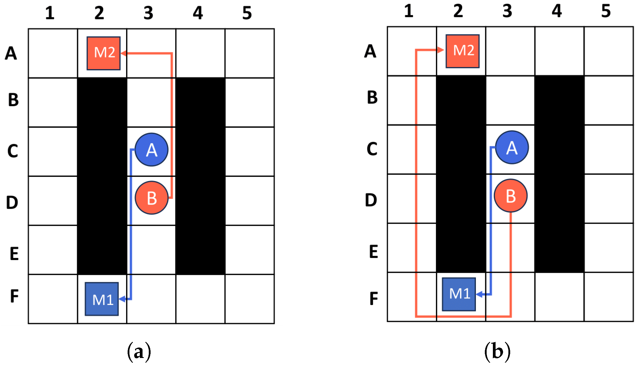
4.2.3. Two Observations

Now, we can use the adaptive windowed ECBS to solve the MAPF problem in a smart factory environment. During the practical experiments, two situations are observed that are worth optimizing, and the following work is based on the two observations.

Observation 1: The number of tasks in the scenario is greater than the number of agents, so there are many abundant tasks unassigned. Abundant tasks create room for optimization and therefore require more sophisticated handling. For agents encountering multiple conflicts in their current tasks, they can choose to perform other available abundant tasks.

Observation 2: During the process of solving TAPF, agents become idle after completing their current tasks. Directly assigning new tasks to these newly idle agents may lead to an unreasonable task assignment scheme. Instead, the task assignment scheme should consider all agents collectively to achieve a better solution, rather than considering the newly idle agent in isolation.

These observed situations occur frequently, and optimizing them is expected to obtain better solutions. Therefore, we propose two optimization strategies: Periodic Conflict Detection Optimization Strategy (PDOS) and Task Swapping Optimization Strategy (TSOS).

Periodic Conflict Detection Optimization Strategy (Observation 1): This optimization is typically for scenarios where the number of tasks is greater than the number of agents. If the number of agents equals the number of tasks, each agent only being able to be assigned a corresponding task is a limitation due to the finite task assignment scheme available. Abundant tasks undoubtedly expand the solution space, providing more options for solutions. For those agents that encounter frequent conflicts during task execution, they can choose to perform other available abundant tasks.

The task assignment phase does not consider potential conflicts between agents, which are resolved during the path planning phase. Frequent conflicts among agents may increase task costs, resulting in the final task cost differing from the one used during task assignment. This is illustrated in Figure 7a, which depicts a local scenario at a certain timestep involving agents A, B, and C, as well as tasks M1, M2, M3, and M4. The task assignment scheme assigns agents A, B, and C to tasks M1, M2, and M3, while task M4 is assigned to the nonexistent virtual agent A4. Once agents A, B, and C complete their respective tasks M1, M2, and M3, the virtual agent A4 will disappear. In the path planning phase (solid line), conflicts can be observed as agents A, B, and C need to pass through a narrow corridor, leading to delays. Assume agent B needs to wait for one timestep, and agent C needs to wait for two timesteps. Conflicts result in the cost for agent C to execute task M3 increasing by 2; however, the extra timesteps provide potential room for optimization. Abundant tasks indicate a larger solution space and the solutions are always expected to have lower path costs. Figure 7b illustrates such possibilities. The abundant task M4 is assigned to agent C, which costs only 5, saving one timestep. By considering conflicts in advance and using the optimal space provided by task M4, the 2 timestep costs incurred by agent C in Figure 7a are eliminated. The dashed line represents the result of the next assignment. The total path cost in Figure 7a is 26 (soc). However, in Figure 7b, the next assignment result only requires 2 additional timesteps, reducing the total path cost to 16 (soc).

Once tasks are assigned, the execution process of the agents will not be interrupted, and only reassign new tasks after completing their current ones. Pre-emptive re-scheduling should be adopted and actively intervened in Figure 7a to enable agent C to execute task M4. A simple periodic check is implemented in our work to avoid an increase in timestep costs. This approach, although very naive, is sufficient to prevent extended timestep costs and allows for optimization through intervention in path planning. For the periodic time, it is set to the same value as the replanning period $\delta$. Before the next iteration of path planning, we update the task costs of agents that encounter conflicts.

The prerequisite for the optimization strategy is that future path information must be known. For this problem, we adopt the adaptive window in path planning, which divides the timesteps into some windows. As a result, it is possible to know some paths for future timesteps. We determine whether an agent encounters a conflict by comparing the cost of the agent executing its current task with the cost $c_{ij}$ cached by the BFS algorithm. If they are different, it indicates that the agent has encountered a conflict. We do not consider situations where a conflict occurs but does not result in an increased path cost. Our focus is solely on situations where conflicts lead to an increase in path costs.

The strategy is implemented in the TaskCostUpdate function (line 27) of the adaptive windowed ECBS algorithm. The details of the TaskCostUpdate function are as follows.

Algorithm 3 TaskCostUpdate

Input: agents A, graph G, map M, path $P_t$   1: for $a_i$ in A do   2:     $c_t\leftarrow$ GetCurrentTaskCost $\left(a_i,P_t\right)$   3:     $c_{ij}\leftarrow$ GetCacheDistance$(a_i,G,M)$   4:      if $c_t$≠$c_{ij}$ then   5:       $c_{ij}\leftarrow c_t$   6:    end if   7: end for   8: if exist agent $a_i$ has updated the task cost then   9:     release the tasks of all agents.   10: end if

(1) Line 2: Obtain the cost of agent $a_i$ performing the current task.

(2) Line 3: Obtain the cached shortest distance cost $c_{ij}$ between the location of agent $a_i$ and the task location.

(3) Lines 4–6: If $c_t$ is not equal to $c_{ij}$, it means that agent $a_i$ has encountered a conflict, and the agent’s current task execution cost needs to be updated.

(4) Lines 8–10: If any agent has updated its task cost, all tasks currently assigned to agents need to be released, awaiting reassignment.

Task Swapping Optimization Strategy (Observation 2): The process of solving the TAPF problem is accompanied by the emergence of new idle agents. The presence of newly idle agents can result in an inappropriate task assignment scheme. Directly assigning a new task to the newly idle agent may not always be the best choice, because swapping tasks with other agents could achieve a lower overall cost. Therefore, we will re-evaluate the task assignment scheme for all agents collectively to achieve a better solution, rather than considering the newly idle agent in isolation. This strategy allows the idle agent to either execute a new task or execute an already assigned task as long as it is not yet finished. This is beneficial when the idle agent can complete the task in fewer timesteps than other agents, and other agents try to assign themselves to a new low-cost task. Consequently, as long as a new idle agent appears, we will consider all agents collectively to achieve a better solution.

For example, in the scenario shown in Figure 8, there are two agents, A and B, and three tasks, M1, M2, and M3, with the initial task assignment scheme being that agent A executes task M1 and agent B executes task M2 (Figure 8a). After agent B completes task M2, if agent B is assigned the new task M3, this will result in a total cost of 8 (Figure 8b). However, if the new task M3 is assigned to agent A and agent B goes to execute the unfinished task M1, the total cost will be 6 (Figure 8c). Swapping the tasks successfully reduces the total cost. This example is common in a smart factory. For example, in an automotive workshop, smart vehicles (agents) deliver different parts and tools to various workstations. Suppose workstations 1, 2, and 3 require a wrench, screws, and paint, respectively, with each smart vehicle storing all these parts and tools. The strategy can be applied to optimize the task assignment scheme. A superior delivery scheme can improve operational efficiency and reduce energy consumption.

The introduction of this strategy presents a unique problem in this paper: the occurrence of invalid paths. Invalid paths arise when an agent’s task is reassigned to another agent during execution, making the agent’s previously planned path invalid. This is because the strategy allows agents to execute tasks that have already been assigned but are not yet completed. The agents originally responsible for these tasks might generate invalid paths, which is a drawback of this strategy. To assess the impact of this drawback on the algorithm’s performance, we conducted evaluations in the Experiments section. Specifically, we analyzed the ratio of invalid paths to total paths and identified the conditions under which invalid paths are likely to occur. The results indicate that the proportion of invalid paths is relatively low and primarily arises when the tasks are insufficient (i.e., the number of agents exceeds the number of tasks), which is considered acceptable.

Before formally introducing the implementation of this strategy, an unmentioned problem in the adaptive WECBS algorithm must first be addressed. The replanning period $\delta$ requires agents to move paths for $\delta$ timesteps in each path planned. However, if the task target location is too close, agents may fail to move for the full $\delta$ timesteps. Thus, agents must be assigned sufficient tasks to ensure the planned path length is at least $\delta$ timesteps. In this strategy, we check whether the current tasks are sufficient to guarantee that the agent moves at least $\delta$ timesteps. If not, additional tasks are assigned and the task assignment considers all agents.

Algorithm 4 CheckTasks

Input: agents A, tasks assignment scheme $\mathcal{T}$, replanning period $\delta$   1: $t\leftarrow$ TaskCompleteMinTime(A, $\mathcal{T}$)   2: $t_n\leftarrow$ current timestep   3: while  $t<t_n+\delta$do   4:     for $a_i$ in A do   5:        set ${\mathit{v}}_i\left(t\right)$ as the initial position for agent $a_i$ in the next task assignment.   6:     end for   7:     Algorithm 1: Multi-Factor Hungarian Assignment.   8:     $t\leftarrow$ TaskCompleteMinTime(A, $\mathcal{T}$)   9: end while   10: start the next iteration of path planning.

This strategy is implemented in the CheckTasks function (line 34) of Algorithm 2. The detailed implementation of the MoveAgents function is outlined below:

(1) Line 1: Calculate the time required for each agent to complete its tasks and select the minimum time to set as t.

(2) Line 2: Obtain now timestep $t_n$.

(3) Lines 3–9: If the currently assigned tasks are insufficient for the agent to move $\delta$ timesteps, additional tasks are assigned. Then, the time t is recalculated.

(4) Line 10: Start the next path planning iteration.

4.3. Overall Algorithm Flow

The TAPF solution proposed in this paper, MTA-AWECBS, has been thoroughly explained in the previous sections. To further improve its clarity, this section will present the entire algorithm flow. Figure 9 details the complete flow of the MTA-AWECBS algorithm.

5. Experiments and Results

In this part, a series of experiments are conducted to evaluate the effectiveness of the proposed algorithm. The primary focus is on the algorithm’s scalability, adaptability, congestion level, and performance across varying parameter settings. First, the algorithm’s scalability directly determines whether it can handle the TAPF problem in complex factory environments. To demonstrate the scalability of our algorithm, Section 5.1 compares the success rates of different algorithms across various map configurations. Next, the algorithm’s adaptability to the factory environment has a direct impact on its execution efficiency. Section 5.2 compares the detailed performance of different algorithms in a real-world factory environment. In addition, Section 5.3 evaluates the performance of the proposed algorithm in reducing traffic congestion level. Lastly, Section 5.4 evaluates the algorithm’s performance under various parameter configurations.

The algorithm MTA-AWECBS is implemented in C++11 and tested on a computer equipped with an Intel i7-8550 CPU and 16 GB of memory. Famous algorithms, including Token Passing (TP) [36], Token Passing with Task Swaps (TPTSs) [36], and Conflict-Based Steiner Search (CBSS) [19] are used for comparison with our method (MTA-AWECBS). Unless otherwise specified, all tests will use the parameters listed in

Table 2. Experimental parameter settings.

Parameter	Value	Meaning
$\eta$	10	time horizon
$\delta$	4	replanning period
$\omega$	1.5	ECBS suboptimal boundary
$D_{max}$	100	maximum travel distance
$N_{max}$	20	maximum number of executable tasks
r	0.5	agent radius
$\alpha$	1.4	window increase factor
$\beta$	0.8	window decrease factor
runtime	60 s	runtime limit

. The initial positions of agents and tasks are randomly generated, with the current system time used as the random seed for initialize. This ensures randomness of both positions and tasks across experiments and enables reproducibility to support future research.

The key evaluation metrics adopted in this paper are ms and soc. Recall that in Section 3, ms (timestep cost) represents the number of timesteps required for all agents to reach their target, while soc (total path cost) represents the total path cost for the agents to complete all tasks. These two metrics effectively reflect the quality of the algorithm.

5.1. Algorithm Scalability and Success Rate

As previously discussed, many algorithms can hardly handle large-scale tasks and agents effectively, resulting in lower solution quality in complex environments. Therefore, the scalability of the algorithm deserves further examination. The algorithm’s scalability is investigated on three widely used maps (Figure 8a), which are sourced from [5]. Each map is a four-connected grid, where each cell is connected to its four neighboring cells (up, down, left, and right). Therefore, the agent can move in any of these four directions or remain in its current position. On each map, the algorithm’s performance is tested in six scenarios where scales are different in the number of tasks and number of available agents. To alleviate the differences caused by the random initialization of agents and tasks, 20 instances are tested for each agent–task combination to compute the algorithm’s average success rate.

The results (Figure 10) clearly show the superior scalability of our algorithm (MTA-AWECBS) across all maps when the number of tasks reaches 100, and its effectiveness remains advantageous as the number of agents grows (up to 30). An overall trend can be observed: as the number of tasks increases, all algorithms except ours exhibit varying degrees of decline in success rate, and the situation worsens further when the number of agents reaches 30. Even in the trivial random map, this trend is still obvious. Not to mention the most complicated maze map, where the success rate shows a sharp decrease. The CBSS algorithm exhibits the most noticeable downward trend, and the possible reason is that the CBSS algorithm focuses on finding the optimal solution, leading to a significant increase in search time. In contrast, our algorithm focuses on suboptimal solutions, which effectively reduces search time.

This experiment clearly shows that our algorithm has good scalability and is able to handle large numbers of tasks and agents.

5.2. Algorithm Adaptability in Smart Factory Environments

Besides success rate, the adaptability of algorithms in the factory environment is also an essential condition, reflected by shorter ms and lower soc. The ms (timestep cost) represents the number of timesteps required for agents to complete all tasks. A shorter timestep implies faster task completion. The soc (total path cost) represents the total path distance required for agents to complete all tasks. A lower path cost indicates lower energy consumption. These two evaluation metrics can effectively reflect the algorithm’s adaptability to the scenario. Tests in this section are conducted using a real factory layout (Figure 11), which includes functional areas such as storage, workstation, and passages. The number of tasks is set to four values: 50, 100, 150, and 200, while the number of agents ranges from 10 to 50. When the algorithm runs successfully, its ms and soc are recorded; if it fails, it is labeled as “Timeout”.

Two overall trends can be observed from

Table 3. The ms and soc for the algorithms TP, TPTS, CBSS, and MTA-AWECBS (our algorithm) in the factory scenario (Figure 11) are presented. When an algorithm runs successfully, its ms and soc are recorded; if it fails, it is marked as “Timeout”.

		TP		TPTS		CBSS		MTA-WECBS
Tasks	Agents	ms	soc	ms	soc	ms	soc	ms	soc
50	10	75	449	44	431	84	312	42	313
	20	64	524	29	561	44	429	22	302
	30	49	570	23	661	35	524	21	386
	40	54	687	22	841	29	687	23	525
	50	62	959	23	1101	Timeout		20	564
100	10	86	655	51	501	119	394	51	465
	20	62	731	31	601	78	516	34	552
	30	65	868	29	811	69	713	26	585
	40	51	1048	26	1001	56	861	23	688
	50	64	1122	25	1095	Timeout		23	835
150	10	86	655	60	591	101	420	63	523
	20	81	842	48	721	86	596	35	605
	30	69	1077	37	894	Timeout		27	682
	40	62	1232	35	1054	Timeout		26	811
	50	65	1524	Timeout		Timeout		25	924
200	10	107	955	83	821	100	504	71	679
	20	89	977	58	912	Timeout		36	630
	30	77	1152	49	1054	Timeout		31	782
	40	71	1282	Timeout		Timeout		28	849
	50	79	1678	Timeout		Timeout		27	1008

: one is that as the number of tasks increases, both ms and soc increase, which is expected, as more tasks lead to greater timesteps and longer paths. The other is that as the number of agents increases, ms decreases while soc increases. The decrease in ms is due to the reduction in task load per agent as their number increases, leading to a lower timestep cost. The rise in soc is attributed to the increased interactions (such as congestion, conflicts, and task competition) among a larger number of agents, as well as their path planning, which leads to higher path costs. Regardless of the specific trend, our algorithm achieves superior adaptability. When the number of agents or tasks increases, the growth of the ms and soc keep within a reasonable range. When only the number of agents increases, the reduction in ms is more pronounced compared to other algorithms. Compared to TP, TPTS, and CBSS, our algorithm reduces ms by an average of 55%, 16%, and 47%, respectively, and soc by an average of 32%, 32%, and 3%. Furthermore, it can also be observed that both TPTS and CBSS algorithms encountered multiple “Timeouts”, especially CBSS, which has a failure rate of approximately 50%. This issue is particularly noticeable in large-scale task and agent scenarios. In contrast, no “Timeout” occurred with our algorithm, further showing its superiority in scalability and adaptability.

Usually, a larger number of agents results in lower ms, because the tasks assigned to each agent decrease. However, the TP algorithm is an exception when the number of agents reaches 50, and the is likely caused by some agents using “dummy paths” to avoid conflicts arising from the large number of agents. It is worth noting that soc of all algorithms increases as the number of agents increases, especially when the number of agents is large, where the increase is more significant. Therefore, infinitely increasing the number of agents for a smaller ms is not a wise strategy. For example, at the scale of 200 tasks, as the number of agents increases from 40 to 50, one can merely observe a 4% reduction in ms; however, this will also cause a 10% increase in soc.

Optimization Strategies: To evaluate the contribution of our two optimization strategies (Periodic Conflict Detection Optimization Strategy and Task Swapping Optimization Strategy) to the adaptability of the MTA-AWECBS algorithm, we conducted experimental comparisons of the differences in ms and soc with and without the optimization strategies. Meanwhile, to properly evaluate the benefits of the optimization strategies, the computational cost (runtime) is also considered. In the experiment, the case where these two optimization strategies are applied is referred to as ‘Two Strategy’, while the case without any optimization strategies applied is referred to as ‘No Strategy’. The experiment continues to use the same factory layout (Figure 11) and tests with different numbers of agents and tasks. The number of tasks is set to four values, 50, 100, 150, and 200, while the number of agents is set to either 10 or 50.

The experiment results (

Table 4. A comparison of the ms and soc for MTA-AWECBS under different numbers of agents and tasks in the factory scenario, with and without the introduction of our two proposed optimization strategies.

		No Strategy			Two Strategies			Optimization Ratio
Tasks	Agents	ms	soc	runtime	ms	soc	runtime	ms	soc
50	10	71	385	9	44	347	9	38%	10%
	50	26	619	10	22	593	11	15%	5%
100	10	63	507	10	53	433	11	15%	15%
	50	35	956	11	25	821	13	28%	15%
150	10	87	686	10	62	579	12	29%	16%
	50	36	1170	13	26	974	15	28%	17%
200	10	90	763	12	75	673	14	17%	12%
	50	35	1202	14	26	1018	18	25%	15%

) clearly show that our two optimization strategies improve the adaptability of MTA-AWECBS, with ms and soc decreasing by averages of 24% and 13%, respectively. With the introduction of the optimization strategies, the maximum increase in computation time remains only 4 s, occurring when there are 200 tasks and 50 agents. This is because a relatively large number of tasks and agents provides more opportunities for the optimization strategies to be effective. Overall, these two optimization strategies enhance the algorithm’s performance while maintaining a reasonable computational time cost. The reason for this improvement is that the first strategy considers all agents collectively to achieve a better solution whenever tasks are assigned; while the second strategy makes full use of abundant tasks to provide better options for potentially conflicting agents.

Invalid Paths: Invalid paths are caused by the introduction of Task Swapping Optimization Strategy (strategy 1), resulting in idle runs of agents that waste energy and increase soc. This is a unique problem caused by our algorithm, and we are responsible for evaluating its impact on the algorithm’s adaptability in real factories. We divide our algorithm into two phases: Phase 1 is the task-abundant phase (i.e., when the number of tasks exceeds the number of agents), while Phase 2 is the task-inabundant phase (i.e., when the number of tasks is fewer than the number of agents). We conducted experiments to collect statistical data for both phases and performed a detailed analysis based on the statistical results, investigating the impact of different phases on the algorithm’s performance and adaptability. The experiment continues to use the factory environment (Figure 11). The number of tasks is set to 100 and 200, while the number of agents varies from 10 to 50.

It is clear from Figure 12 that invalid paths mainly occur in Phase 2, particularly when the number of agents reaches 50, with more than 70% of invalid paths concentrated in this phase. This is because the presence of many idle agents (Phase 2) increases competition for tasks, generating more invalid paths. Additionally, as the number of tasks increases from 100 to 200, the total proportion of invalid paths significantly decreases. Both Phase 1 and Phase 2 show a reduction in invalid paths. This is because the increase in the number of tasks leads to longer total path lengths, but the growth of invalid paths is shorter than the total path length. Therefore, as long as there are enough tasks, the proportion of invalid paths is expected to decrease further. This perfectly fits a real factory environment, where a large number of abundant tasks further reduce the proportion of invalid paths.

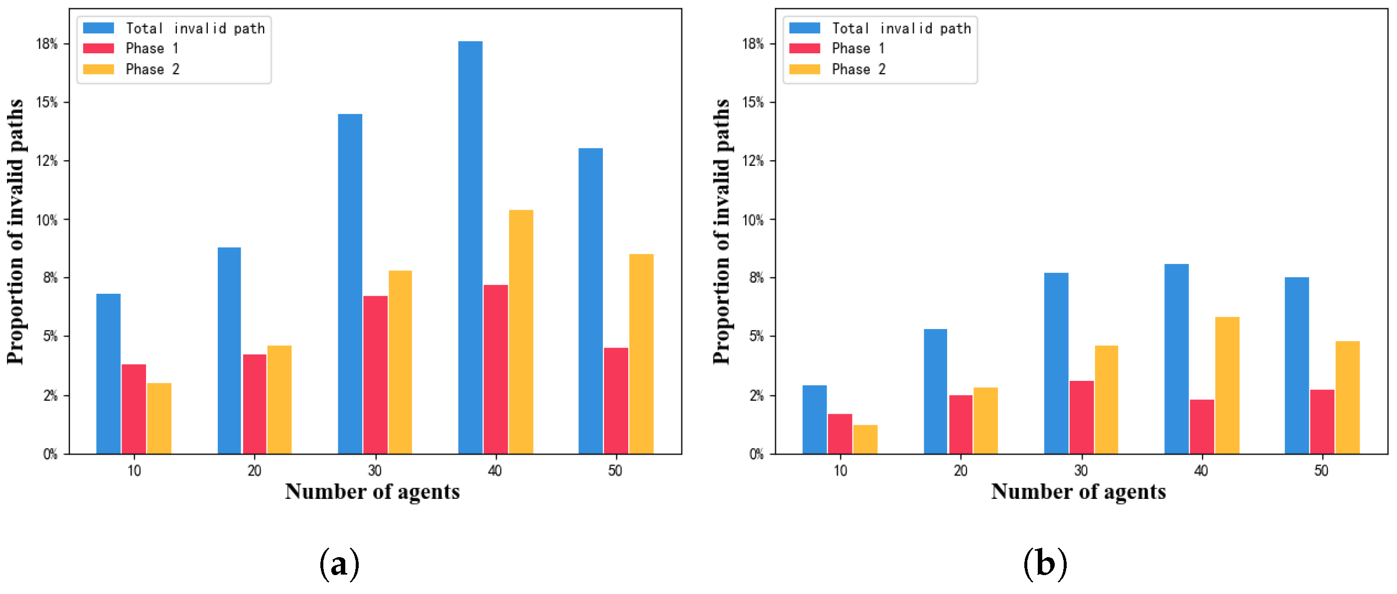
5.3. Congestion Level Test

Traffic congestion levels directly impact throughput, while the throughput reflects the operational efficiency of agents. To alleviate traffic congestion and avoid deadlock, a new mathematical description of global congestion level is proposed. Building upon this definition, an adaptive window is introduced to optimize the WECBS algorithm. Therefore, it is necessary to conduct experimental validation to evaluate the performance of the proposed algorithm in alleviating traffic congestion. The effectiveness of this approach is evaluated by observing changes in congestion levels after incorporating the adaptive window into the ECBS algorithm. The experiment continues to use the real factory layout (Figure 11), randomly assigning tasks to each agent and simulating 100 timesteps. This means that each agent will continue performing the task until it has moved for 100 timesteps. The number of agents grows from 10 to 50. The initial time horizon $\eta$ and replanning window $\delta$ are both set to 10.

The experimental results (Figure 13) clearly show that the adaptive window greatly alleviates congestion levels, achieving an average reduction of 31%. As the number of agents increases, the congestion level also continues to rise. Without the adaptive window (WECBS), the congestion level peaked at 160; however, as a result of introducing the adaptive window (adaptive WECBS), the maximum congestion level remained below 100, greatly alleviating the traffic congestion problem.

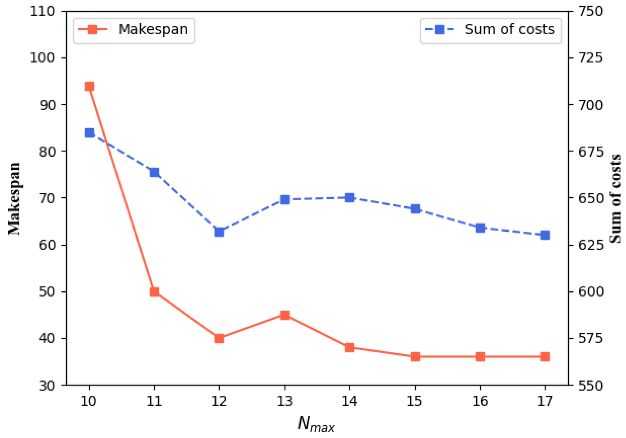
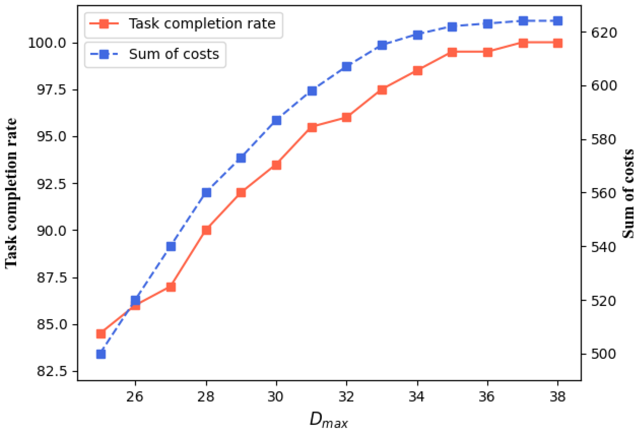
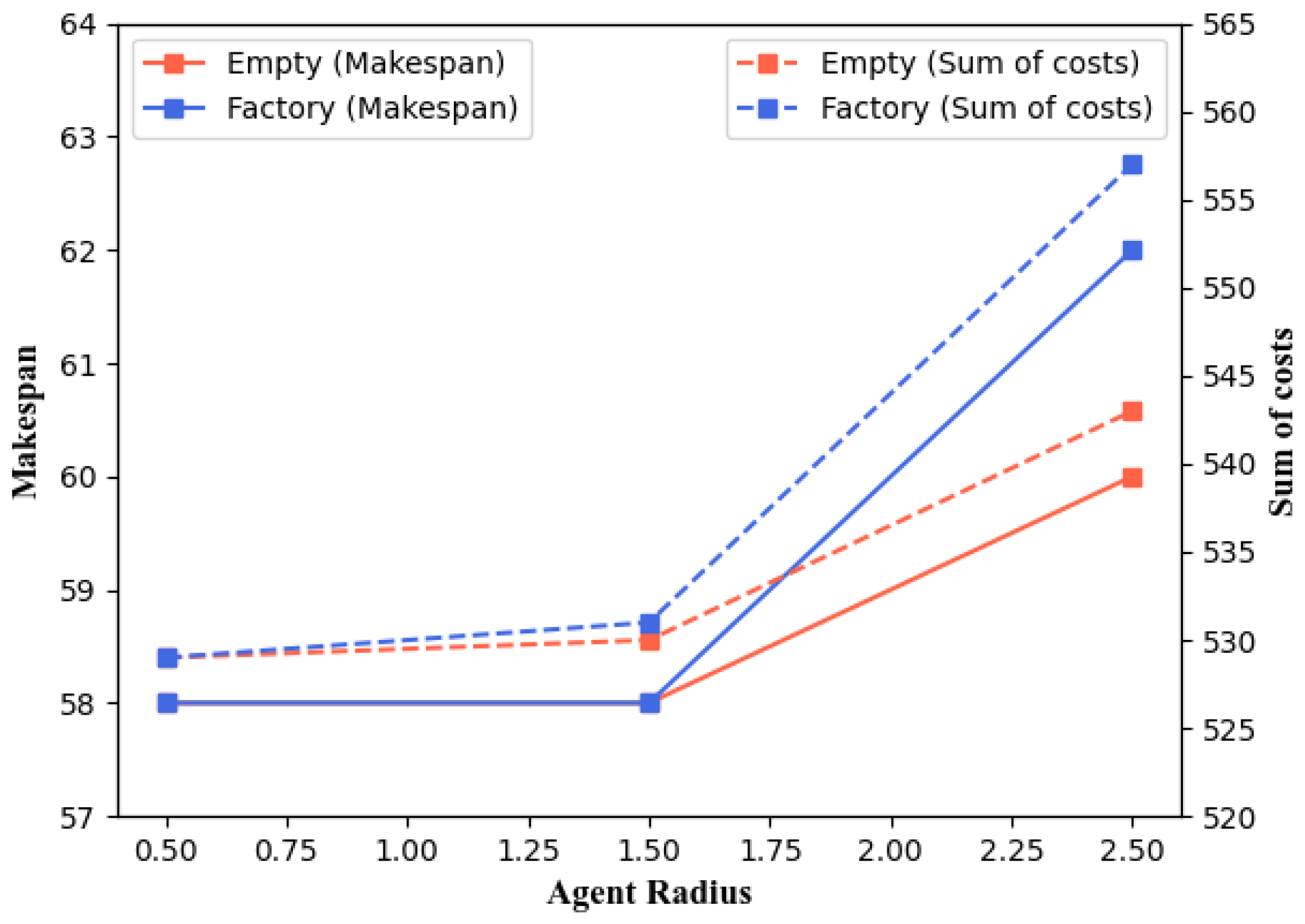
5.4. Parameter Settings for Agents

Through comparison with other algorithms, we have shown the advantages of our proposed algorithm MTA-AWECBS. Its performance under different parameter settings has yet to be explored. In this section, the performance of MTA-AWECBS will be investigated under different parameter settings.

Maximum number of executable tasks constraint $N_{max}$: First, we tested the impact of the maximum number of tasks $N_{max}$ on the algorithm’s results. The experiment is conducted in the factory scenario (Figure 11), in which 200 tasks and 20 agents are initialized. In this experiment, the value of $N_{max}$ must not be too small; otherwise, not all tasks can be completed. Therefore, the minimum value of $N_{max}$ is set to 10.

The experimental results (Figure 14) show that $N_{max}$ can influence the algorithm’s performance, particularly in the early stages of $N_{max}$ growth (10 to 12), where ms and soc exhibit a rapid decline. Specifically, the ms decreases by approximately 58%, while the soc decreases by about 22%. When $N_{max}$ reaches 15, ms and soc gradually stabilize. In practical factory production, $N_{max}$ is widely used in smart factories to balance task assignment, such as material delivery and parts delivery. By moderately setting a limit on the maximum number of executable tasks, the efficiency of the agents can be ensured, preventing excessive workload.

Maximum travel distance $D_{max}$: In addition to exploring the maximum number of executable tasks, the maximum travel distance $D_{max}$ is another key parameter. The experiment is still conducted on the factory map (Figure 11), with 200 tasks and 20 agents initialized. This experiment primarily focuses on the task completion rate and soc under different $D_{max}$ settings. The task completion rate is expressed as the ratio of the number of completed tasks to the total number of tasks.

The experimental results are shown in Figure 15; both the task completion rate and soc increase as $D_{max}$ increases. During the $D_{max}$ initial growth (25–28), soc exhibits a linear increase, because most agents have reached their maximum travel distance $D_{max}$, yet have not completed all tasks. When $D_{max}$ exceeds 28, soc exhibits a slow, nonlinear increase, because some agents have completed all assigned tasks and no longer need to fully utilize $D_{max}$, thereby reducing unnecessary path consumption. For the task completion rate, it steadily increases until $D_{max}=36$, at which point all agents have completed their assigned tasks. In real factory environments, $D_{max}$ is also a key factor, because agents are usually constrained by battery resources or signal range, which directly influence the operation efficiency.

Agent volume: The volume of agents is one of the key challenges addressed in this paper. It is necessary to verify its effectiveness and evaluate the impact of different agent radii r on the algorithm’s performance. Two different maps are used in the experiment: a 37 × 90 empty map and a 37 × 90 factory map, both configured with 70 tasks and 10 agents.

The experimental results (Figure 16) show that our algorithm is capable of handling the path planning problem with agent volume. However, as the agent radius increases, the algorithm faces new scalability challenges, particularly when the agent’s radius is 2.5, which leads to a significant increase in both the ms and soc. The new scalability challenges caused by the agent radius are what we are currently investigating to solve. Additionally, the agent volume has a more significant impact in the complex factory scenario. The ms and soc in the factory map are higher than the empty map. The difference is especially pronounced when the agent radius is 2.5. This is because the factory map is irregular and complex, requiring higher path costs.

6. Discussion

This paper investigates the multi-agent task assignment and path planning problem in a real factory environment and proposes an effective solution to the TAPF problem. Unlike previous studies, this research focuses on solving problems under real constraints and in large-scale scenarios. The experimental results demonstrate that our method effectively handles large-scale scenarios and greatly reduces the global congestion level. This advantage is attributed to the introduction of the adaptive window, designed based on the global congestion definition we proposed. For the definition of congestion level, some studies describe the congestion level by agents occupying the same shared edge [16], while many other studies measure the congestion level using area density [46] or probabilistic approaches [47]. These methods can effectively reflect congestion in relatively simple scenarios, but in large-scale and complex scenarios, they may encounter issues such as increased computational overhead and the inability to precisely measure congestion. For example, in large-scale scenarios, due to the inherently high density, relying solely on density to measure congestion often lacks accuracy. This paper assesses the congestion level of the scenario by calculating the difference between the actual distance traveled by the agent and the shortest path. If an agent does not choose the shortest path, it indicates interactions with other agents (such as conflicts or detours). This method offers a simple yet effective way to reflect the overall congestion level of the scenario. Based on this definition of congestion, this paper introduces an adaptive window. This adaptive window can dynamically adjust time horizon $\eta$ according to the current congestion level of the scenario, enabling fast and efficient path planning.

Although this study focuses on the factory environment, the proposed TAPF solution is also applicable to other complex scenarios. First, experimental results demonstrate that the algorithm operates stably even in intricate maze maps without any failures. Second, the complexity of factory maps is higher compared to typical warehouse scenarios. Warehouse scenarios are generally more symmetrical and simpler, far less complex than factory environments. Additionally, factory maps includes various environmental features, such as storage areas and production lines. Therefore, the algorithm is capable of effectively addressing multi-agent task assignment and path planning challenges across different types of scenarios. However, this study has certain limitations, as it is designed for static environments. If new obstacles (such as dropped goods) appear during the agent delivery process, it could affect the algorithm’s effectiveness. Therefore, the proposed algorithm is better suited for environments that are relatively complex and static.

7. Conclusions

In this paper, the problem of multi-agent task assignment and path planning in smart factory environments is investigated, and a novel algorithm called MTA-AWECBS is proposed, consisting of two components: task assignment and path planning. In task assignment, not only is the distance factor considered, but several other factors are also taken into account to effectively solve the problem of task assignment. In path planning, the algorithm considers the volume geometry of agents and introduces an adaptive window based on windowed ECBS to effectively address traffic congestion and deadlock problems. Furthermore, two commonly overlooked situations that frequently arise in the TAPF problem are addressed, which further improves the algorithm’s performance.

The experimental results show that our proposed algorithm MTA-AWECBS consistently maintains a high success rate in various map scenarios (e.g., intricate maze map), without encountering any failures due to timeouts, demonstrating good scalability. Moreover, the algorithm exhibits high adaptability, as it performs better in large-scale factory environments (e.g., 200 tasks and 50 agents), achieving an average 39% reduction in timestep cost (Makespan) and an average 22% reduction in total path cost (Sum of costs) compared to contemporary TAPF algorithms. This improvement can be attributed to the adaptive window introduced in Algorithm 2: AWECBS, which effectively solves deadlocks, reduces congestion level by an average of 31%, and thus increases throughput, ultimately enhancing the algorithm’s efficiency in large-scale scenarios. Furthermore, the two optimization strategies (Algorithm 3 and Algorithm 4) introduced in this paper contribute to further enhancing the overall performance of the algorithm.

This study only focuses on static factory environments and does not consider dynamic changes in the scenario, such as new tasks, new agents, and dynamic obstacles. These are potential challenges in smart factories. Another noteworthy problem is the scalability challenge arising from agent geometry, which is one of the primary focuses of our current research.

References

1. Wu, K.; Xu, J.; Zheng, M. Industry 4.0: Review and proposal for implementing a smart factory. Int. J. Adv. Manuf. Technol. 2024, 133, 1331–1347. [Google Scholar] [CrossRef]
2. Wang, S.; Wan, J.; Zhang, D.; Li, D.; Zhang, C. Towards smart factory for Industry 4.0: A self-organized multi-agent system with big data based feedback and coordination. Comput. Netw. 2016, 101, 158–168. [Google Scholar] [CrossRef]
3. Dorri, A.; Kanhere, S.S.; Jurdak, R. Multi-Agent Systems: A Survey. IEEE Access 2018, 6, 28573–28593. [Google Scholar] [CrossRef]
4. Khamis, A.; Hussein, A.; Elmogy, A. Multi-robot Task Allocation: A Review of the State-of-the-Art. Coop. Robot. Sens. Netw. 2015, 604, 31–51. [Google Scholar] [CrossRef]
5. Stern, R.; Sturtevant, N.; Felner, A.; Koenig, S.; Ma, H.; Walker, T.; Li, J.; Atzmon, D.; Cohen, L.; Kumar, T.; et al. Multi-agent pathfinding: Definitions, variants, and benchmarks. In Proceedings of the International Symposium on Combinatorial Search, Napa, CA, USA, 16–17 July 2019; Volume 10, pp. 151–158. [Google Scholar]
6. Ma, H.; Koenig, S. Optimal target assignment and path finding for teams of agents. In Proceedings of the 2016 International Conference on Autonomous Agents and Multiagent Systems, Singapore, 9–13 May 2016; pp. 1144–1152. [Google Scholar]
7. Bai, X.; Cao, M.; Yan, W.; Ge, S.S. Efficient routing for precedence-constrained package delivery for heterogeneous vehicles. IEEE Trans. Autom. Sci. Eng. 2019, 17, 248–260. [Google Scholar] [CrossRef]
8. Qian, T.; Liu, X.F.; Zhan, Z.H.; Yong, J.; Zhang, Q.; Duan, D.; Mao, C.; Tang, Y. A Multiobjective Ant Colony System for Multi-Agent Pickup and Delivery. In Proceedings of the 2024 11th International Conference on Machine Intelligence Theory and Applications (MiTA), Melbourne, Australia, 14–23 July 2024; pp. 1–8. [Google Scholar]
9. Kim, G.; Jeong, Y. An approximation algorithm for mobile multi-agent monitoring and routing problem. Flex. Serv. Manuf. J. 2025, 1–27. [Google Scholar] [CrossRef]
10. Hönig, W.; Kiesel, S.; Tinka, A.; Durham, J.; Ayanian, N. Conflict-based search with optimal task assignment. In Proceedings of the International Joint Conference on Autonomous Agents and Multiagent Systems, Stockholm, Sweden, 10–15 July 2018; pp. 757–765. [Google Scholar]
11. Tang, Y.; Ren, Z.; Li, J.; Sycara, K. Solving multi-agent target assignment and path finding with a single constraint tree. In Proceedings of the 2023 International Symposium on Multi-Robot and Multi-Agent Systems (MRS), Boston, MA, USA, 4–5 December 2023; pp. 8–14. [Google Scholar] [CrossRef]
12. Chen, Z.; Alonso-Mora, J.; Bai, X.; Harabor, D.D.; Stuckey, P.J. Integrated Task Assignment and Path Planning for Capacitated Multi-Agent Pickup and Delivery. IEEE Robot. Autom. Lett. 2021, 6, 5816–5823. [Google Scholar] [CrossRef]
13. Kudo, F.; Cai, K. A TSP-Based Online Algorithm for Multi-Task Multi-Agent Pickup and Delivery. IEEE Robot. Autom. Lett. 2023, 8, 5910–5917. [Google Scholar] [CrossRef]
14. Li, J.; Tinka, A.; Kiesel, S.; Durham, J.W.; Kumar, T.S.; Koenig, S. Lifelong multi-agent path finding in large-scale warehouses. In Proceedings of the AAAI Conference on Artificial Intelligence, Vancouver, BC, Canada, 2–9 February 2021; Volume 35, pp. 11272–11281. [Google Scholar]
15. Song, S.; Na, K.I.; Yu, W. Anytime Lifelong Multi-Agent Pathfinding in Topological Maps. IEEE Access 2023, 11, 20365–20380. [Google Scholar] [CrossRef]
16. Chen, X.; Feng, L.; Wang, X.; Wu, W.; Hu, R. A Two-Stage Congestion-Aware Routing Method for Automated Guided Vehicles in Warehouses. In Proceedings of the 2021 IEEE International Conference on Networking, Sensing and Control (ICNSC), Xiamen, China, 5–7 November 2021; Volume 1, pp. 1–6. [Google Scholar] [CrossRef]
17. Henkel, C.; Abbenseth, J.; Toussaint, M. An Optimal Algorithm to Solve the Combined Task Allocation and Path Finding Problem. In Proceedings of the 2019 IEEE/RSJ International Conference on Intelligent Robots and Systems (IROS), Macau, China, 3–8 November 2019; pp. 4140–4146. [Google Scholar] [CrossRef]
18. Ren, Z.; Rathinam, S.; Choset, H. MS*: A New Exact Algorithm for Multi-agent Simultaneous Multi-goal Sequencing and Path Finding. In Proceedings of the 2021 IEEE International Conference on Robotics and Automation (ICRA), Xi’an, China, 30 May–5 June 2021; pp. 11560–11565. [Google Scholar] [CrossRef]
19. Ren, Z.; Rathinam, S.; Choset, H. CBSS: A New Approach for Multiagent Combinatorial Path Finding. IEEE Trans. Robot. 2023, 39, 2669–2683. [Google Scholar] [CrossRef]
20. Liu, M.; Ma, H.; Li, J.; Koenig, S. Task and path planning for multi-agent pickup and delivery. In Proceedings of the International Joint Conference on Autonomous Agents and Multiagent Systems (AAMAS), Montreal, QC, Canada, 13–17 May 2019; pp. 1152–1160. [Google Scholar]
21. Kuhn, H.W. The Hungarian method for the assignment problem. Nav. Res. Logist. 2004, 52, 7–21. [Google Scholar] [CrossRef]
22. Xu, Q.; Li, J.; Koenig, S.; Ma, H. Multi-Goal Multi-Agent Pickup and Delivery. In Proceedings of the 2022 IEEE/RSJ International Conference on Intelligent Robots and Systems (IROS), Kyoto, Japan, 23–27 October 2022; pp. 9964–9971. [Google Scholar] [CrossRef]
23. Pisinger, D.; Ropke, S. Large neighborhood search. In Handbook of Metaheuristics; Springer: Cham, Switzerland, 2019; pp. 99–127. [Google Scholar] [CrossRef]
24. Bai, Y.; Kanellakis, C.; Nikolakopoulos, G. SA-reCBS: Multi-robot task assignment with integrated reactive path generation. IFAC-PapersOnLine 2023, 56, 7032–7037. [Google Scholar] [CrossRef]
25. Xu, X.; Yin, Q.; Quan, Z.; Ju, B.; Miao, J. Heuristic-Based Task Assignment and Multi-Agent Path Planning for Automatic Warehouses. In Proceedings of the 2023 China Automation Congress (CAC), Chongqing, China, 17–19 November 2023; pp. 1490–1495. [Google Scholar] [CrossRef]
26. Chen, L.; Liu, W.L.; Zhong, J. An efficient multi-objective ant colony optimization for task allocation of heterogeneous unmanned aerial vehicles. J. Comput. Sci. 2022, 58, 101545. [Google Scholar] [CrossRef]
27. Bai, X.; Fielbaum, A.; Kronmüller, M.; Knoedler, L.; Alonso-Mora, J. Group-Based Distributed Auction Algorithms for Multi-Robot Task Assignment. IEEE Trans. Autom. Sci. Eng. 2023, 20, 1292–1303. [Google Scholar] [CrossRef]
28. Hoffman, K.L.; Padberg, M.; Rinaldi, G. Traveling salesman problem. Encycl. Oper. Res. Manag. Sci. 2013, 1, 1573–1578. [Google Scholar] [CrossRef]
29. Sharon, G.; Stern, R.; Felner, A.; Sturtevant, N.R. Conflict-based search for optimal multi-agent pathfinding. Artif. Intell. 2015, 219, 40–66. [Google Scholar] [CrossRef]
30. Surynek, P. Multi-goal multi-agent path finding via decoupled and integrated goal vertex ordering. In Proceedings of the AAAI Conference on Artificial Intelligence, Online, 2–9 February 2021; Volume 35, pp. 12409–12417. [Google Scholar] [CrossRef]
31. Andreychuk, A.; Yakovlev, K.; Surynek, P.; Atzmon, D.; Stern, R. Multi-agent pathfinding with continuous time. Artif. Intell. 2022, 305, 103662. [Google Scholar] [CrossRef]
32. Cohen, L.; Uras, T.; Kumar, T.S.; Xu, H.; Ayanian, N.; Koenig, S. Improved Solvers for Bounded-Suboptimal Multi-Agent Path Finding. In Proceedings of the Twenty-Fifth International Joint Conference on Artificial Intelligence (IJCAI), New York, NY, USA, 9–15 July 2016; pp. 3067–3074. [Google Scholar]
33. Li, J.; Ruml, W.; Koenig, S. Eecbs: A bounded-suboptimal search for multi-agent path finding. In Proceedings of the AAAI Conference on Artificial Intelligence, Online, 2–9 February 2021; Volume 35, pp. 12353–12362. [Google Scholar]
34. Ma, H.; Harabor, D.; Stuckey, P.J.; Li, J.; Koenig, S. Searching with consistent prioritization for multi-agent path finding. In Proceedings of the AAAI conference on artificial intelligence, Honolulu, HI, USA, 29–31 January 2019; Volume 33, pp. 7643–7650. [Google Scholar]
35. Luna, R.; Bekris, K.E. Push and swap: Fast cooperative path-finding with completeness guarantees. In Proceedings of the Twenty-Second International Joint Conference on Artificial Intelligence (IJCAI), Barcelona, Spain, 16–22 July 2011; pp. 294–300. [Google Scholar]
36. Ma, H.; Li, J.; Kumar, T.; Koenig, S. Lifelong multi-agent path finding for online pickup and delivery tasks. In Proceedings of the 16th Conference on Autonomous Agents and MultiAgent Systems, Sao Paulo, Brazil, 8–12 May 2017; pp. 837–845. [Google Scholar]
37. Fang, C.; Mao, J.; Li, D.; Wang, N.; Wang, N. A coordinated scheduling approach for task assignment and multi-agent path plannin. J. King Saud Univ.-Comput. Inf. Sci. 2024, 36, 101930. [Google Scholar] [CrossRef]
38. Li, K.; Yan, X.; Han, Y. Multi-mechanism swarm optimization for multi-UAV task assignment and path planning in transmission line inspection under multi-wind field. Appl. Soft Comput. 2024, 150, 111033. [Google Scholar] [CrossRef]
39. Huo, X.; Wu, X. Task and intelligent path planning algorithm for teams of AGVs based on multi-stage method. In Proceedings of the 2021 IEEE 4th International Conference on Automation, Electronics and Electrical Engineering (AUTEEE), Shenyang, China, 19–21 November 2021; pp. 517–523. [Google Scholar] [CrossRef]
40. Wagner, G.; Choset, H. Subdimensional expansion for multirobot path planning. Artif. Intell. 2015, 219, 1–24. [Google Scholar] [CrossRef]
41. Nguyen, V.; Obermeier, P.; Son, T.; Schaub, T.; Yeoh, W. Generalized target assignment and path finding using answer set programming. In Proceedings of the International Symposium on Combinatorial Search, Napa, CA, USA, 16–17 July 2019; Volume 10, pp. 194–195. [Google Scholar]
42. Okumura, K.; Défago, X. Solving simultaneous target assignment and path planning efficiently with time-independent execution. Artif. Intell. 2023, 321, 103946. [Google Scholar] [CrossRef]
43. Shimizu, T.; Taneda, K.; Goto, A.; Hattori, T.; Kobayashi, T.; Takamido, R.; Ota, J. Offline Task Assignment and Motion Planning Algorithm Considering Agent’s Dynamics. In Proceedings of the 2023 9th International Conference on Automation, Robotics and Applications (ICARA), Abu Dhabi, United Arab Emirates, 10–12 February 2023; pp. 239–243. [Google Scholar] [CrossRef]
44. Bundy, A. Breadth-first search. In Catalogue of Artificial Intelligence Tools; Springer: Berlin/Heidelberg, Germany, 1986; p. 13. [Google Scholar] [CrossRef]
45. Kumar, A. A modified method for solving the unbalanced assignment problems. Appl. Math. Comput. 2006, 176, 76–82. [Google Scholar] [CrossRef]
46. Ge, Z.; Jiang, J.; Coombes, M. A congestion-aware path planning method considering crowd spatial-temporal anomalies for long-term autonomy of mobile robots. In Proceedings of the 2023 IEEE International Conference on Robotics and Automation (ICRA), London, UK, 29 May–2 June 2023; pp. 7930–7936. [Google Scholar] [CrossRef]
47. Street, C.; Lacerda, B.; Mühlig, M.; Hawes, N. Multi-Robot Planning Under Uncertainty with Congestion-Aware Models. In Proceedings of the 2016 International Conference on Autonomous Agents and Multiagent Systems, Singapore, 9–13 May 2020; pp. 1314–1322. [Google Scholar]
Figure 1. An illustration of conflict types. (a) Vertex conflict. (b) Edge conflict.
Electronics 14 00842 g001
Figure 2. Conflict considers agent volume.
Electronics 14 00842 g002
Figure 3. The figure illustrates a conflict scenario involving agents with real volume. The radius of agent A (blue) is 2.5, and the radius of agent B (red) is 1.5. Although located at different positions, a collision still occurs due to overlapping occupied cells.
Electronics 14 00842 g003
Figure 4. Conflict detection considering the volume of agents.
Electronics 14 00842 g004
Figure 5. The fixed time horizon in windowed ECBS leads to the occurrence of deadlocks. (a) Time horizon η = 2. (b) Time horizon η = 4.
Electronics 14 00842 g005
Figure 7. The figure shows a case of the Periodic Conflict Detection Optimization Strategy. The solid lines represent the current assignment results, while the dashed lines represent the next task assignment. (a) Agents A, B, and C encounter conflicts while passing through a narrow corridor. Assuming agent B waits for one timestep and agent C waits for two timesteps. The cost for agent C to execute task M3 increases from 4 to 6. The total path cost is 26. (b) The abundant task M4 is assigned to agent C, which costs only 5. The total cost is 16.
Electronics 14 00842 g007
Figure 8. The figure shows a case of the Task Swapping Optimization Strategy. (a) Agents A and B execute tasks M1 and M2. (b) After agent B completes task M2, it becomes idle and is assigned task M4, resulting in a total cost of 8. (c) Agent B executes the unfinished task M1, while agent A switches to execute task M3, reducing the total cost to 6.
Electronics 14 00842 g008
Figure 9. Flow chart of MTA-AWECBS algorithm.
Electronics 14 00842 g009
Figure 10. The success rate results for the algorithms TP, TPTS, CBSS, and MTA-AWECBS (our algorithm) in different scenarios. The colors correspond to different algorithms and the X-axis represents the number of tasks.
Electronics 14 00842 g010
Figure 11. A real factory map, where black squares represent obstacles, and the other squares represent empty spaces.
Electronics 14 00842 g011
Figure 12. The proportion of invalid paths produced by MTA-AWECBS with varying numbers of agents and tasks: (a) 100 tasks and (b) 200 tasks.
Electronics 14 00842 g012
Figure 13. The level of traffic congestion for adaptive WECBS and WECBS with varying numbers of agents in the factory scenario.
Electronics 14 00842 g013
Figure 14. The performance of MTA-AWECBS under different configurations of the maximum number of executable tasks.
Electronics 14 00842 g014
Figure 15. The performance of MTA-AWECBS under different configurations of the maximum travel distance.
Electronics 14 00842 g015
Figure 16. The performance of MTA-AWECBS under different agent volume sizes. The dashed lines represent Makespan, and the solid lines represent Sum of Costs.
Electronics 14 00842 g016