Abstract
The increasing integration of distributed energy resources into distribution feeders introduces significant uncertainties, stemming from volatile renewable sources and other fluctuating electrical elements, which pose substantial challenges for optimal power flow (OPF) analysis. This paper introduces a data-driven distributionally robust chance-constrained (DRCC) approach to address the stochastic Alternating Current (AC) OPF problem in distribution grids, where the exact probability distributions of uncertainties are unknown. The proposed method utilizes the Wasserstein metric to construct an ambiguity set based on empirical distributions derived from historical data, eliminating the need for prior knowledge of the underlying probability distributions. Notably, the size of the Wasserstein ball within the ambiguity set is inversely related to the volume of available data, allowing for adaptive robustness. Moreover, a computationally efficient reformulation of the DRCC-OPF model is developed using the LinDistFlow AC power flow approximation. The effectiveness and precision of the developed method are validated through multiple IEEE distribution test cases, demonstrating higher reliability of the security constraints compared with other methods. As more data become available, this reliability is systematically and securely adjusted to achieve greater economic efficiency.
1. Introduction
Due to the characteristics of low voltage and scalability of the distribution network, the distribution network integrates large-scale variable renewable energy, which is evolving from the traditional power grid to active distribution networks. However, with the increase in its penetration rate, the volatility and intermittency of renewable energy power generation have brought great risks to the security, stable operation, and control of the power grid [1,2], also providing distribution system operators with more management and control means [3]. In addition, uncertainty significantly impacts distribution networks in various real-world scenarios. For example, urban business districts experience substantial load variations between weekdays and weekends, leading to inefficiencies and increased fault risks. Offshore wind farms face instability due to fluctuating wind speeds, causing voltage fluctuations that can disrupt electrical equipment and affect system reliability. Therefore, reducing or eliminating the influence of uncertainty on the distribution network is of great significance in achieving the utilization of renewable energy and the optimal allocation of resources.
The optimal power flow (OPF) problem aims to optimize an objective function by regulating controllable devices, primarily generators, while adhering to operational constraints [4,5]. With the increasing impact of uncertainties such as grid fluctuations and load deviations, these uncertainties become significant factors in OPF analysis. Consequently, research shifts towards addressing uncertain OPF, focusing on stochastic OPF [6,7,8] and robust OPF [9,10,11,12] under conditions like forecast errors and load fluctuations. Stochastic OPF typically assumes that uncertainties follow a known single or mixed probability distribution and uses probabilistic information (e.g., expectation, variance) to convert the stochastic problem into a deterministic one. For instance, in [8], prediction errors assume a Gaussian distribution, and the problem reformulates into a tractable form using chance-constrained Alternating Current (AC) OPF with semidefinite programming. However, the true underlying distribution is often unknown and may not be easily described by a single distribution. Considering only expectations can lead to issues such as overvoltage and overload during large transient fluctuations, posing significant risks to grid operations. On the other hand, robust OPF does not rely on specific probability distributions; instead, it constructs an ambiguity set from collected data to describe uncertainty and uses duality to transform the problem into its robust counterpart. In [11], a multi-period AC OPF efficiently solves by applying convex relaxation, setting a budget uncertainty set for loads, a dynamic uncertainty set for renewable generation, and developing an adaptive robust optimization model. While robust OPF strategies withstand all possible scenarios, they often do so at the expense of economic efficiency, resulting in overly conservative solutions.
Due to the low reliability of stochastic optimization and the conservativeness of robust optimization, Distributionally Robust Optimization (DRO) [13,14,15,16,17] emerges as a solution. DRO places the true distribution within an ambiguity set, constructs this set based on distributional characteristics, and analyzes the worst-case distribution within it. This approach develops a control strategy applicable to all distributions in the ambiguity set without being overly conservative. Importantly, DRO is data-driven and does not require precise probabilistic information. The construction of the ambiguity set is crucial, directly affecting the model’s accuracy and reliability. Various methods exist for constructing ambiguity sets in DRO problems [18], including Kullback–Leibler (KL) divergence, Jensen–Shannon (JS) divergence, moment-based methods, and Wasserstein distance. KL and JS divergences are ineffective when distributions are far apart or have heavy tails. Moment-based ambiguity sets are popular due to their simplicity and ease of handling. For instance, historical data estimate the first- and second-order moments of the true distribution, which are reformulated using second-order cone programming (SOCP) for bilateral distributionally robust chance constraints, transforming the problem into a tractable convex program [19]. In [20], a feasible approximation method uses moment information to reformulate the distributionally robust chance-constrained OPF problem into a deterministic one, employing optimized Bonferroni approximation to reduce solution conservativeness. However, expectation and variance alone do not fully capture the true distribution. Ideally, the amount of data should be inversely proportional to the conservatives of solutions, that is, less data should lead to more conservative solutions. This property aligns with real-world scenarios, but moment-based ambiguity sets lack this characteristic.
As an alternative, the Wasserstein metric, grounded in optimal transport theory, measures the distance between probability distributions by calculating the minimal cost of transforming one into another. The Wasserstein ambiguity set extends this concept, creating uncertainty sets to model distributional uncertainty in robust optimization. Since the strategy obtained from Wasserstein-metric-based Distributionally Robust Optimization (WDRO) has better reliability as well as performance guarantees for finite samples, it is used in fields such as machine learning [21], econometrics [22], and various optimization applications [23,24,25]. In [26], product prices are modeled as ambiguity sets based on the Wasserstein metric for optimizing the planning operations of an oil refinery. The DRO method uses the Wasserstein distance to solve the optimal reactive power dispatch problem with chance constraints under second-order cone programming and linear power flow models in [27]. A real-time scheduling method for solving distributionally robust chance constraints under generation forecast errors is proposed in the literature [28], where the quadratic constraints are relaxed by reconstructing linear techniques, and a linear reconstruction is constructed to transform the problem into a deterministic one. The work in [29] minimizes the expected value of the quadratic cost function under the system response reflected by the exact AC power flow model and the approximate linear power flow model and ensures that the opportunity constraint is satisfied. DRO is more applied under convex relaxation as well as linearized models for OPF problems, while convex relaxation may have large optimality gaps that seriously deviate from the feasible region of the original problem, and more seriously, it does not have industrial-grade applications. The linear model has been widely used because of its high computational efficiency and ideal programming. Practically speaking, system operators prefer the linear market clearing model due to the transparency of its solution. However, there is little literature devoted to the special structure of distribution networks, and sometimes intractable constraints are ignored [30]. Moreover, there are large errors when applying Direct Current (DC) OPF in distribution networks, which may jeopardize the market efficiency, so this paper uses an alternative linearization method.
This paper addresses the challenges posed by uncertainties in distribution grids due to the increasing integration of distributed energy resources, particularly volatile renewable sources. We propose a data-driven distributionally robust chance-constrained (DRCC) approach to solve the stochastic AC OPF problem in such grids:
- This paper introduces a DRCC approach that employs the Wasserstein metric to construct an ambiguity set from historical data, eliminating the need for prior knowledge of probability distributions.
- A computationally efficient reformulation of the DRCC-OPF model is presented using the LinDistFlow AC power flow approximation, reducing computational costs despite varying data volumes.
- The proposed method is validated through multiple IEEE distribution test cases, demonstrating higher reliability of the security constraints compared with existing methods.
The rest of this paper is organized as follows: Section 2 defines the DRO model for the chance-constrained OPF. Section 3 reformulates the DRO problem by transforming it into a deterministic linear optimization problem. Section 4 presents the case study of the distribution grid, deriving the advantages of the WDRO method over other treatments, and finally, conclusions are drawn in Section 5.
2. Preliminaries and Problem Statement
In this section, we first fix the notations and introduce some basic concepts of graph theory. The problem statement of interest is then presented in a constructive way. In particular, the optimal power flow problem of distribution networks in the presence of uncertainties is taken into account using a distributionally robust chance-constrained formulation.
2.1. Notations and Basic Graph Theory
The symbol represents the column vector of all ones with appropriate dimensions. We use calligraphy font to represent a set and boldface font to represent a vector. For a vector , its upper and lower bounds are denoted as and , respectively. Let be the true distribution and be the expectation under distribution . For a given support , denotes the set of all probability distributions with support . For an arbitrarily given set , is equal to the cardinality of the set. Throughout this article, we will use the notion of the tilde diacritic over the letter for uncertain variables.
Let be a graph, in which and are the set of all nodes and edges, respectively. The symbol represents the set of nodes other than the root node 0 in the tree graph, i.e., . The sets of parent and child nodes associated with each node are denoted by and . For the graph of the tree, each nonroot node has a unique ancestor and a set of children nodes except the so-called “leaf” nodes which have no children nodes.
2.2. Network Representation and Power Flow Equation
Electric power systems are typically modeled as networks of buses interconnected by branches. Buses serve as physical points to which various electronic components, such as generators, loads, storage units, and shunt impedances, are connected. Branches, on the other hand, provide pathways for the flow of electrical current between buses. This article examines an N-bus radial distribution system, represented by a tree-like graph , where buses correspond to nodes in the set , and a branch from bus i to bus j is denoted by edge . It is well established that in a radial distribution network without isolated nodes, the number of nodes exceeds the number of branches by one, i.e., . Each branch is characterized by resistance , reactance , and an upper bound on apparent power flow . Without loss of generality, the root node 0 is designated as the slack bus, which connects the distribution side to the transmission side, commonly referred to as the substation. Consequently, the set of nonroot buses is .
Each system bus is specified by its voltage magnitude , voltage phase , net active power and net reactive power , such that
where and represent net demand for active and reactive power injection on the node, whereas and are controllable active and reactive power injections for the buses associated with generators. Unless otherwise specified, it is assumed that the power flowing out from the reference bus 0 is known, together with p.u. and , where is the voltage phase of root node bus 0. Obviously, the power flowing out from node j is equal to zero if and one has if there is no generator attached to the node . Figure 1 provides a concrete interpretation for the introduced notations, where .
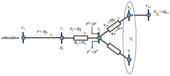
Figure 1.
Illustrative example of the main notations in radial distribution grids.
This article employs the branch flow model to characterize the AC power flow balance in radial distribution grids, as it demonstrates superior numerical stability compared with the bus injection model [31]. The branch flow equation is expressed as follows:
where () represents active(reactive) power flow of branch , and is denoted as the square of voltage magnitude, i.e., for . It is worth noting that Equations (2a) and (2b) mean the power balance of nonroot nodes , while Equation (2c) characterizes the voltage balance of nonroot nodes . It is well known that the branch flow model (3) fully characterizes the power flows for a balanced radial network [31].
2.3. Optimal Power Flow Problem of Distribution Networks
The OPF problem is a cornerstone in the planning and operation of distribution systems. Its primary objective is to minimize a specified function, typically encompassing generation costs and power losses, while ensuring that all operational constraints are satisfied within safe limits.
However, the nonlinearity inherent in the AC power flow model (3) introduces a nonconvex structure to the OPF problem, making it challenging to solve directly with guaranteed convergence. To address this, linear approximation or convex relaxation techniques are commonly employed. Among these, the DC power flow model has been widely used for linearizing OPF problems in transmission networks, where the resistance-to-inductance ratio of transmission lines is negligible, and reactive power flows are supplied locally. Nevertheless, this DC linearization approach is unsuitable for distribution networks, as the resistance-to-inductance ratio in such systems is significantly larger.
Different from the DC-like linearization technique, we employ an AC optimal power formulation for radial distribution systems based on the so-called LinDistFlow model [32], which provides an alternative linear approximation for the branch flow model (3) by neglecting the real and reactive power losses but accounting for apparent flows and voltage magnitudes. Specifically, the LinDistFlow has the following form:
which is a linear form of Equation (3).
To effectively tackle the challenges of solving nonconvex OPF problems in a distributed manner, one approach is to convexify the OPF problem before applying distributed algorithms. A common technique for convexification is second-order cone programming (SOCP) relaxation. However, this method often struggles to accurately represent the original nonconvex problem, ensuring optimality primarily in simpler network configurations, such as IEEE benchmark systems and acyclic radial networks. Furthermore, SOCP solvers typically require significant computational resources, limiting their scalability for large transmission networks with thousands of buses and meshed topologies. As a computationally efficient alternative, the LinDistFlow method provides a convex approximation of power flow equations. Numerical simulations, as cited in [33], demonstrate that LinDistFlow is well suited for a wide range of distribution circuits, offering a viable solution with reduced complexity.
To this end, the full OPF problem associated with the LindistFlow model is given by
where the quadratic form is used in (4a) by giving the cost coefficients associated with the controllable generators at bus . Moreover, the remaining inequality constraints (4c)–(4f) represent, respectively, engineering limits on the voltage magnitudes, power injections, and magnitudes of apparent power in distribution networks.
2.4. DRCC-OPF of AC Distribution Networks
Since the uncertainties derived from volatile renewable and fluctuating loads increasingly emerge in distribution feeders, the deterministic LinDistFlow-based OPF model (4) is no longer available to guide the planning and operation of distribution systems. For simplicity of exposition, we restrict our attention to the case of uncertainties induced by renewable energy generation because this consideration is sufficient to illustrate the proposed techniques but is technically much simpler than the general case. Nevertheless, the explored results in this article can be easily extended to any case of uncertainties involving fluctuating load consumption and volatile energy reserve capacities.
More specifically, the net power injections (1) in the presence of random active and reactive generations and become
In order to describe explicitly the uncertainty propagation across the distribution grid, we distinguish the unpredictable renewable energy production as follows:
where correspond to conventional active and reactive power generation, whereas represent volatile renewable feed-in such that
in which active and reactive power , respond to the fixed forecasting amount associated with renewable generation, and random forecasting errors , characterize the impact of uncertainties on node j. Note that different from only concerning random forecasting errors derived from active power generation in [29], the randomness of reactive power is also taken into account in this article.
When accounting for uncertainty, controllable generating units are responsible for compensating the total deviations arising from forecast errors in renewable generation. Consequently, the random active and reactive power generations, and , in (5), can be reformulated as
where and are the vector of active and reactive power prediction error, respectively. Here, with a slight abuse of notation, and stand for the forecasting active and reactive power injection from generators on node j. Moreover, the decision variable in (8) determines to what extent the controllable generators on node j are involved in compensating for renewable generation deviations, which satisfies if there is no generator on node j and .
Next, it is essential to examine the expressions for edge power flows and nodal voltages influenced by the uncertainty in renewable power production. To aid in this derivation, we introduce two indicator matrices, and , with components that satisfy the following conditions:
As a consequence of the notations in (9) and Formulas (5)–(7), the propagation of uncertainty stemming from fluctuating renewable generation across the distribution network can be captured by the stochastic LinDistFlow model in the following vector-based form:
where are column vectors representing the random active and reactive power flows, and , across branch , where . The column vectors contain the elements for nonroot buses . The vector includes the random counterparts of the squared voltage magnitudes for all . The constant matrices are diagonal, containing and for each branch , where . Clearly, when the prediction error in renewable power generation vanishes, i.e., , the conditions of Equations (10a)–(10c) reduce to the power flow balance system (3a)–(3c) at the nominal operating point.
Thanks to Equations (10a)–(10c), the uncertain active and reactive edge power flows and squared voltage magnitudes with respect to (8) lead to
where is the remaining matrix formed by removing the first column of . Matrices are deterministic counterparts of in the absence of uncertainties. Notably, the Equations (11a)–(11c) give rise to the fact that voltage and the power outflow from slack bus 0 maintain constant whatever the uncertainties emerge or not. More importantly, the system response models concerning (8), (11a)–(11c) are all in a linear manner with respect to renewable power prediction derivations.
In addition to guaranteeing the compensation of power production deviation from the forecast values, the controllable generators must ensure various soft constraints of inequalities (4c)–(4f) in a prescribed high probability, which leads to the following chance-constrained formulations:
where , which typically take small values in practice, are referred to as the violation probability of chance-constrained optimizations with respect to squared voltage magnitudes, power generations, and squared magnitudes of apparent powers, respectively.
The stochastic OPF problem with chance constraints aims to find feasible solutions within a confidence region defined by specified probability levels. This requires comprehensive knowledge of the probability distribution of the random variables and , which is essential for the existence of optimal solutions. However, in practice, these precise distributions are typically unavailable. Instead, only a finite set of historical data is accessible, which provides some reliable probabilistic information. Consequently, deriving the true distributions needed to formulate the expected cost and chance constraints from finite samples is challenging, leading to ambiguity in these distributions.
To effectively manage the uncertainties inherent in probability distributions and assess their impact on power flows and voltage limits, this study emphasizes a data-driven distributionally robust chance-constrained optimal power flow (DRCC-OPF) model, formulated as follows:
where represents the decision variables, and the ambiguity set encompasses all admissible probability distributions inferred from accessible historical data. The objective function (13a) is defined as the worst-case expectation of generation costs concerning the probability distributions within the ambiguity set . Constraint (13b) ensures that the cumulative participation factors of power generation from renewable sources sum to 1. The equality constraints (13c) enforce the balance of active and reactive power at the nominal operating point, where renewable power generation precisely matches forecasted values. Furthermore, the distributionally robust chance constraints (13d)–(13g) ensure the adequacy of voltage quality, active power, reactive power, and transmission line capacity, respectively.
The data-driven DRCC-OPF problem (13), incorporating the objective function (13a) and chance constraints (13d)–(13g), is designed to account for the worst-case probability distribution within the ambiguity set . This approach ensures robust performance across various ambiguous distributions contained in . The optimization framework utilizes upper and lower bounds, such as , , , , , , and , alongside confidence probability factors , , , and , to quantify the reliability and performance levels of uncertain variables. Consequently, the primary objective of the optimization problem (13) is to identify a data-driven (sub-)optimal solution that achieves high reliability with minimal certification requirements.
2.5. Wasserstein Metric and Ambiguity Set
The true probability distribution of uncertain renewable energy generation deviations, denoted as , is not precisely known but is assumed to reside within an ambiguity set constructed from a finite set of historical data. This study employs the Wasserstein metric to define the ambiguity set, encompassing all probability distributions that are proximate to a nominal or empirical distribution with respect to a predefined probability metric [15].
Specifically, given a set of historical samples , the empirical probability distribution is expressed as
where represents the Dirac measure centered at . This empirical distribution serves as an approximation of the true distribution . As the volume of historical data increases indefinitely, the “distance” between and diminishes according to the prescribed probability metric, indicating convergence of to as . The Wasserstein metric is utilized in this study to quantify the distance between and .
Definition 1
(Wasserstein Metric [34]). The Wasserstein metric between two arbitrary probability distributions and within the space is defined as
where Π denotes a joint distribution of the random variables and , with and as their respective marginals.
It is remarkable that the Wasserstein metric in (14) holds for arbitrarily , but we preferably employ the -norm in this article because of its appealing advantages in numerical computation. As a result of giving N historical samples and the set of all probability distributions under support , the Wasserstein-metric-based ambiguity set of the true distribution can be described by the following formulation:
which is also referred to as a Wasserstein ball with the empirical distribution as the center and r as the radius.
Obviously, the radius of the Wasserstein ball, which has been known as an inverse function with respect to the amount of historical data, plays an essential role in the performance of the data-driven DRCC-OPF problem (13). As shown in [35] by giving a confidence level and the diameter B of the support , a possible radius can be obtained as
which nevertheless leads to a conservative choice. In the recent work in [29], the radius formula
has been proved to save significant conservation and thus provide desirable performance for the DRO in numerical tests. Here, the constant C is obtained by solving the following optimization problem:
where is the mean value of historical samples. In particular, the radius given in (17) degenerates to the case of (16) while setting .
3. Data-Driven Distributionally Robust Optimization via the Wasserstein Metric
In this section, we elaborate on the reformulation of the proposed data-driven DRCC-OPF problem to a tractable mathematical program that enables us to solve with off-the-shelf optimization and analysis tools.
3.1. Worst-Case Evaluation of Objective Function
To facilitate a tractable reformulation of the data-driven DRCC-OPF problem (13), we first need to evaluate the worst-case expected costs in the objective function (13a).
More specifically, the quadratic form function in the worst-case expectation of system-wide generation cost of (13a) can be rewritten by
where we denote for convenience. Note that the coefficient is constantly greater than zero. Since the expectation and variance are unknown, the strong duality of the Wasserstein ball is used for simplification.
In the Wasserstein ball [15] , the upper semi-continuous convex function is equivalent in the given sample set and the support to
where .
Due to the quadratic form of with respect to the variable y, the maximum point can only occur at three positions, i.e.,
taking the upper approximation to equation (21a), we can obtain
it can be reduced again to
3.2. Linear Approximation of the Branch Flow Limits
Due to the presence of a squared term in the existence probability, it is difficult to use a linear treatment, so linearization is used to approximate the nonlinear constraint. There are various linearization methods for approximating the constraint of a circle, such as rough approximation [36], as well as exact approximation [37]. To improve the approximation performance, an exact approximation is taken here. The nonlinear constraints inside the operator in (13g) can be written as follows:
where a segmented linearization method is used to divide nonlinear constraints into multiple segments of linear constraints.
Finally, (24) can be converted to linear representations with respect to and , and also linearly with respect to , and the number of constraints is changed from to , where denotes the number of nodes in the set . All the nonlinear constraints can be written in matrix form as
where , , and is the confidence to quantify the reliability and performance levels of uncertain variables. It describes the upper bound of the transmission line capacity. Thus, all the constraints become linear constraints with random variables, and the problem can be directly reduced to a deterministic linear optimization problem, which is treated by the method in Section 3.3.
3.3. Reformulation of DRCC-OPF Model
To transform the chance constraints into a form that is both deterministic and tractable, it is necessary to reformulate them appropriately. Constraints involving inf-operators and random variables are inherently nonconvex, posing significant challenges in deriving a tractable form. The generic forms of linear constraints, such as those in (13d)–(13f) and (25), can be expressed in the following standard format:
where and represent affine mappings of the random vectors , and I is the number of all conditions.
According to the results of the work in [38], if the ambiguity set is defined as a vector space using Wasserstein measures, the linear constraint can be reformulated as , in which
where v, , and are auxiliary variables, and denotes the dual norm of .
Given that the Wasserstein ambiguity set is based on the L1 norm, the dual-norm relationship implies . According to the lemma, the number of auxiliary variables increases with the sample size. To mitigate the computational burden associated with large sample sizes, a relaxation is proposed as follows:
Taking the voltage constraint as an illustrative example (a similar methodology applies to all other linear constraints), the voltage constraint (13d) can be reformulated as
where , , and . These correspond to and in Lemma 2, specified as follows:
where denotes the j-th row of the matrix . In summary, by replacing the worst-case expected cost in (13a) with (23), and approximating all inequality chance constraints using (29), the objective function and constraints involving random variables are transformed into a deterministic linear optimization problem. This reformulated problem is amenable to solution via existing interior point method solvers.
4. Case Study
This section presents numerical experiments conducted on two test systems: the modified IEEE 15-bus and 141-bus radial distribution systems in MATPOWER. MATPOWER is an open-source toolbox based on MATLAB R2022b, which is specially used for power systems research and optimization tasks such as power flow calculation, optimal power flow analysis, and economic scheduling. These experiments aim to demonstrate the efficacy of the proposed method. The flowchart in Figure 2 shows the sequence of operations based on the proposed WDRO. The performance of the WDRO approach is evaluated in comparison with three other methods. All simulations are executed using IPOPT within the CasADi framework [39] on a personal computer equipped with an Intel Xeon E5 CPU and 32GB RAM.
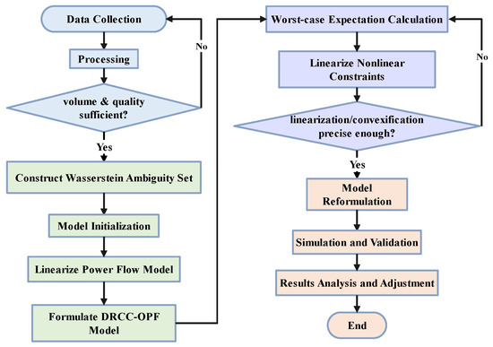
Figure 2.
The flowchart of the sequence of operations.
4.1. IEEE 15-Bus System
The IEEE 15-bus system [40] is utilized with specific modifications: two controllable generators and two wind farms are added. The active power capacities of these generators are set at 1 MW, with lower limits of 0.2 MW and 0 MW, respectively. The reactive power capacity ranges from −1 MVAR to 1 MVAR. The system topology is depicted in Figure 3. The forecasted active power generation for the wind farms denoted as and , is 0.3 MW, while the reactive power generation, and , is 0.3 MVAR. For generating historical data, it is assumed that the random variables follow a multivariate Gaussian distribution with a mean of zero and a standard deviation of 0.06. The confidence level is set at , and the risk parameters are . The selection of these values is based on their use in MATPOWER, where reasonable upper and lower bounds, along with perturbations, are introduced to facilitate the application of the proposed algorithm. These values serve as both numerical examples and representations of a specific grid structure, while also being sufficiently representative of real-world scenarios.
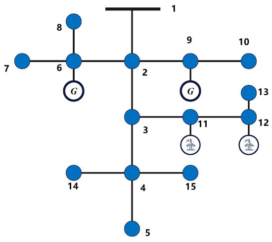
Figure 3.
Topology diagram of IEEE 15-bus system.
Three comparative methods are employed to comprehensively evaluate the performance of the WDRO method, including aspects such as out-of-sample performance, reliability, and variation patterns with sample size.
The first method is Stochastic Programming (SP), which assumes that uncertainties follow a single Gaussian distribution . This approach aims to minimize the expected objective function. The chance constraint is reformulated as , allowing it to be solved using a quadratic conic reformulation. The second method is robust optimization (RO), which mandates that all possible values of the random variable must satisfy the security constraints, ensuring robustness against uncertainty. The third method is Moment-based Distributionally Robust Optimization (MDRO), which constructs an ambiguity set based on the given mean and variance. The security constraint is simplified through a convex reformulation of the two-sided chance constraint using second-order cone programming (SOCP).
Figure 4 illustrates the evolution of operation costs for different methods as a function of sample size. The operation cost is calculated based on in (4a) with the coeffients and ; and and . The RO method disregards probabilistic information about uncertainty, resulting in the highest operation cost, indicative of its conservative strategy. In contrast, the SP method assumes the random variable follows a single known distribution, leading to the lowest operation cost and representing the most optimistic strategy. Moment-based MDRO method reduces conservativeness by incorporating assumptions about the first and second-order moments of the distribution, thus yielding operation costs between those of RO and SP. However, the operation costs for these three methods remain largely unaffected by the amount of historical data. In contrast, WDRO does not assume a specific probability distribution. Instead, it bases its control strategy solely on historical data. When data are scarce, the strategy of WDRO is more conservative, akin to RO. As the data volume increases, WDRO becomes less conservative, approaching the cost efficiency of SP, and highlighting the data-driven nature. Table 1 provides detailed experimental results across different sample sizes, demonstrating that the radius of the Wasserstein ball is inversely related to the sample size; both the radius and the total cost decrease as more data become available. These results indicate that with more data, which provides richer probabilistic information and a clearer distribution, the proposed WDRO approach yields more optimistic solutions.
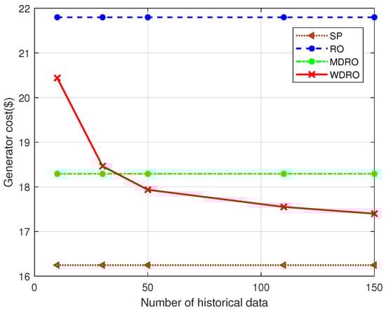
Figure 4.
Total cost evolves with samples under different models.

Table 1.
Evolution of the parameters with sample number.
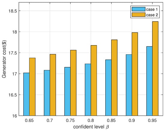
The control strategy is influenced not only by the amount of historical data but also significantly by the method chosen for calculating the radius and the selected confidence level . Figure 5 illustrates the operation costs under various conditions with a sample size of . The figure reveals that employing the original radius calculation method results in a more conservative strategy; moreover, the operation cost escalates with an increase in the confidence level , irrespective of whether the original or improved radius is used. This trend occurs because a higher confidence level expands the radius, thereby encompassing more potential distributions, which leads to a more conservative solution and an associated rise in cost. Consequently, the degree of conservatism in the strategy can be modulated by adjusting the confidence level .
In addition, Table 2 presents the control strategies derived under various conditions with a sample size of . The table highlights the distinct approaches employed for handling power flow constraints, detailing each parameter alongside the associated costs. This complexity underscores the challenge of directly substituting the original primal nonlinear constraints, as each method’s nuanced treatment of constraints leads to unique parameter configurations and cost implications. When selecting a model and control strategy, it is crucial to consider not only the operation cost but also the out-of-sample performance and reliability of the strategy. Table 3 evaluates the out-of-sample performance of different methods using 100 test samples from the same dataset. The data-driven WDRO demonstrates superior out-of-sample performance, evidenced by a smaller standard deviation compared with RO, SP, and MDRO. The reliability of the security constraints across all methods is assessed using Monte Carlo simulations with an additional samples, as shown in Table 4. RO achieves the highest reliability, albeit at the expense of increased operation costs. Conversely, while SP achieves the lowest operating cost, its reliability is compromised due to the significant discrepancy between the assumed Gaussian distribution and the potential actual distribution. Both MDRO and WDRO maintain high reliability while ensuring lower operating costs. Notably, the reliability of the WDRO method decreases as the amount of historical data increases, reflecting a shift towards greater economic efficiency. Thus, the WDRO method offers a favorable balance between reliability and economic performance.
Table 2.
Different Approximation Methods for Constraints.
Table 3.
Out-of-sample performance testing of different approaches.
Table 4.
Reliability under Monte Carlo simulation.
4.2. IEEE 141-Bus System
This section focuses on the modified IEEE 141-bus system to further validate the effectiveness of the proposed method. The system incorporates eight controllable generators at nodes 7, 21, 39, 42, 55, 63, 94, and 119, with active power limits ranging from 0.1 MW to 2 MW and reactive power limits from −2 MVAR to 2 MVAR. Additionally, five wind farms are installed at nodes 13, 30, 50, 91, and 126, each with predicted active and reactive power outputs of 1 MW and 1 MVAR, respectively. The remaining parameters and system topology are referenced in [40]. For historical data generation, it is assumed that the random variable follows a multivariate Gaussian distribution with a mean of 0 and a standard deviation of .
Table 5 presents the total operation cost for different confidence levels with a sample size of . As increases from to , the operation cost of WDRO rises gradually. This trend occurs because, with a fixed sample number N and constant C, a higher results in a larger radius. Consequently, the likelihood of encompassing the true probability distribution increases, leading to higher operating costs and increased conservativeness. Figure 6 illustrates the reliability results of various methods. It is evident that RO, MDRO, and WDRO satisfy the reliability requirements. Although reliability diminishes as the data volume increases, it remains within acceptable limits.
Table 5.
Out-of-sample performance testing of different approaches.
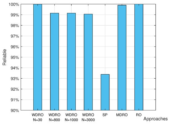
Figure 6.
Reliable of the IEEE 141-bus test system.
To verify whether the voltage of each bus in the IEEE 141-bus system remains within acceptable boundaries, the maximum voltage values for each node across various methods are compiled in Table 6. The table reveals that the WDRO method results in more node voltages concentrated near the reference voltage compared with other methods. This concentration indicates a damping effect on grid fluctuations, making the approach more compatible with power equipment in the distribution network, thereby demonstrating superior voltage performance.
Table 6.
Voltage result under different approaches.
4.3. Computation Time
The computation time of this method primarily consists of two components: the problem construction time and the solution time. To further assess the scalability of the proposed method, computation times were compared across different cases, as shown in Table 7. The results indicate that computation time increases with the number of samples N and is significantly longer for the IEEE 141-bus system compared with the IEEE 15-bus system. Although the computational efficiency of the method can be improved, there is potential for employing distributed computing to accelerate the process. The developed method aligns with the operational requirements of energy networks by providing robust solutions for power flow optimization under uncertainty, thus allowing integration into real-time scheduling processes to support DER management. For trading intervals of real-world energy management in distribution networks, the proposed method is compatible with typical market operations, such as 15 min or hourly intervals, as it provides solutions that can be quickly calculated and updated with new data. Future work will explore multi-timescale optimization to further enhance its applicability in real-world energy trading and management scenarios.
Table 7.
Computation time (s) for different systems.
5. Conclusions and Future Work
The challenges posed by the high penetration of renewable energy sources in the operation and management of distribution systems have been addressed through the development of a data-driven distributionally robust chance-constrained optimal power flow method. This approach leverages the LinDistFlow approximation model of the distribution network, avoiding assumptions about uncertainty and instead relying solely on existing historical data to construct the uncertainty set. The problem is reformulated into a manageable linear programming problem using strong duality theory and conditional value-at-risk approximation. Case studies indicate that as more data become available, the method yields increasingly optimistic solutions. Additionally, the conservativeness of the solution can be modulated by adjusting the confidence level, effectively mitigating the impact of uncertainty compared with other methods. This approach demonstrates superior out-of-sample performance and reliability, enabling distribution system operators to balance economic efficiency with system reliability effectively. However, as distributed energy resource penetration increases, the performance of the proposed method may depend on the availability of sufficient historical data to construct reliable ambiguity sets. Future research directions are proposed to enhance the adaptability and computational efficiency of the method under scenarios with highly distributed energy resource penetration.
Future work will explore the integration of a large network of distributed energy resources, such as battery energy storage systems, plug-in electric vehicles, and flexible loads, into the proposed framework. The goal is to solve the stochastic optimal power flow problem in a fully distributed manner, enhancing scalability and adaptability in complex power systems.
Author Contributions
Conceptualization, F.L. (Fangzhou Liu) and D.X.; methodology, F.L. (Fangzhou Liu) and J.H.; validation, F.L. (Fengfeng Liu) and D.L.; formal analysis, F.L. (Fengfeng Liu) and D.L.; writing—original draft preparation, F.L. (Fangzhou Liu) and J.H.; writing—review and editing, F.L. (Fengfeng Liu), D.L. and D.X. All authors have read and agreed to the published version of the manuscript.
Funding
This research was funded in part by the National Natural Science Foundation of China under grant numbers 6237312 and 62173147.
Institutional Review Board Statement
Not applicable.
Data Availability Statement
The data that support the findings of this study are available from the corresponding author upon reasonable request.
Conflicts of Interest
The authors declare no conflicts of interest.
References
- Impram, S.; Nese, S.V.; Oral, B. Challenges of renewable energy penetration on power system flexibility: A survey. Energy Strategy Rev. 2020, 31, 100539. [Google Scholar] [CrossRef]
- Khalid, M. Smart grids and renewable energy systems: Perspectives and grid integration challenges. Energy Strategy Rev. 2024, 51, 101299. [Google Scholar] [CrossRef]
- Roald, L.A.; Pozo, D.; Papavasiliou, A.; Molzahn, D.K.; Kazempour, J.; Conejo, A. Power systems optimization under uncertainty: A review of methods and applications. Electr. Power Syst. Res. 2023, 214, 108725. [Google Scholar] [CrossRef]
- Yang, C.; Sun, Y.; Zou, Y.; Zheng, F.; Liu, S.; Zhao, B.; Wu, M.; Cui, H. Optimal power flow in distribution network: A review on problem formulation and optimization methods. Energies 2023, 16, 5974. [Google Scholar] [CrossRef]
- Peng, Q.; Low, S.H. Distributed optimal power flow algorithm for radial networks, I: Balanced single phase case. IEEE Trans. Smart Grid 2016, 9, 111–121. [Google Scholar] [CrossRef]
- Louca, R.; Bitar, E. Stochastic AC optimal power flow with affine recourse. In Proceedings of the 2016 IEEE 55th Conference on Decision and Control, Las Vegas, NV, USA, 12–14 December 2016; pp. 2431–2436. [Google Scholar]
- Usman, M.; Capitanescu, F. A stochastic multi-period AC optimal power flow for provision of flexibility services in smart grids. In Proceedings of the 2021 IEEE Madrid PowerTech, Madrid, Spain, 28 June–2 July 2021; pp. 1–6. [Google Scholar]
- Venzke, A.; Halilbasic, L.; Markovic, U.; Hug, G.; Chatzivasileiadis, S. Convex relaxations of chance constrained AC optimal power flow. IEEE Trans. Power Syst. 2017, 33, 2829–2841. [Google Scholar] [CrossRef]
- Zhang, J.; Cui, M.; He, Y.; Li, F. Multi-Period Two-Stage Robust Optimization of Radial Distribution System with Cables Considering Time-of-Use Price. J. Mod. Power Syst. Clean Energy 2022, 11, 312–323. [Google Scholar] [CrossRef]
- Jabr, R.A.; Karaki, S.; Korbane, J.A. Robust multi-period OPF with storage and renewables. IEEE Trans. Power Syst. 2014, 30, 2790–2799. [Google Scholar] [CrossRef]
- Lorca, A.; Sun, X.A. The adaptive robust multi-period alternating current optimal power flow problem. IEEE Trans. Power Syst. 2017, 33, 1993–2003. [Google Scholar] [CrossRef]
- Lee, D.; Turitsyn, K.; Molzahn, D.K.; Roald, L.A. Robust AC optimal power flow with robust convex restriction. IEEE Trans. Power Syst. 2021, 36, 4953–4966. [Google Scholar] [CrossRef]
- Gao, R.; Kleywegt, A. Distributionally robust stochastic optimization with Wasserstein distance. Math. Oper. Res. 2023, 48, 603–655. [Google Scholar] [CrossRef]
- Zhai, J.; Jiang, Y.; Zhou, M.; Shi, Y.; Chen, W.; Jones, C.N. Data-Driven Joint Distributionally Robust Chance-Constrained Operation for Multiple Integrated Electricity and Heating Systems. IEEE Trans. Sustain. Energy 2024, 15, 1782–1798. [Google Scholar] [CrossRef]
- Mohajerin Esfahani, P.; Kuhn, D. Data-driven distributionally robust optimization using the Wasserstein metric: Performance guarantees and tractable reformulations. Math. Program. 2018, 171, 115–166. [Google Scholar] [CrossRef]
- Li, Y.; Han, M.; Shahidehpour, M.; Li, J.; Long, C. Data-driven distributionally robust scheduling of community integrated energy systems with uncertain renewable generations considering integrated demand response. Appl. Energy 2023, 335, 120749. [Google Scholar] [CrossRef]
- Nie, J.; Yang, L.; Zhong, S.; Zhou, G. Distributionally robust optimization with moment ambiguity sets. J. Sci. Comput. 2023, 94, 12. [Google Scholar] [CrossRef]
- Lin, F.; Fang, X.; Gao, Z. Distributionally Robust Optimization: A review on theory and applications. Numer. Algebr. Control Optim. 2022, 12, 159. [Google Scholar] [CrossRef]
- Xie, W.; Ahmed, S. Distributionally robust chance constrained optimal power flow with renewables: A conic reformulation. IEEE Trans. Power Syst. 2017, 33, 1860–1867. [Google Scholar] [CrossRef]
- Yang, L.; Xu, Y.; Sun, H.; Wu, W. Tractable Convex Approximations for Distributionally Robust Joint Chance Constrained Optimal Power Flow under Uncertainties. IEEE Trans. Power Syst. 2021, 37, 1927–1941. [Google Scholar] [CrossRef]
- Engelmann, J.; Lessmann, S. Conditional Wasserstein GAN-based oversampling of tabular data for imbalanced learning. Expert Syst. Appl. 2021, 174, 114582. [Google Scholar]
- Yuan, Y.; Song, Q.; Zhou, B. A Wasserstein distributionally robust chance constrained programming approach for emergency medical system planning problem. Int. J. Syst. Sci. 2022, 53, 2136–2148. [Google Scholar] [CrossRef]
- Arrigo, A.; Ordoudis, C.; Kazempour, J.; De Grève, Z.; Toubeau, J.F.; Vallée, F. Wasserstein distributionally robust chance-constrained optimization for energy and reserve dispatch: An exact and physically-bounded formulation. Eur. J. Oper. Res. 2022, 296, 304–322. [Google Scholar] [CrossRef]
- Nguyen, H.T.; Choi, D.H. Distributionally robust model predictive control for smart electric vehicle charging station with V2G/V2V capability. IEEE Trans. Smart Grid 2023, 14, 4621–4633. [Google Scholar] [CrossRef]
- Dai, X.; Chen, C.; Wang, J.; Fan, S.; Yin, S. A Distributionally Robust Chance-Constrained Offering Strategy for Distributed Energy Resources in Joint Energy and Frequency Regulation Markets. Electr. Power Syst. Res. 2025, 238, 111106. [Google Scholar] [CrossRef]
- Zhao, J.; Zhao, L.; He, W. Data-driven Wasserstein distributionally robust optimization for refinery planning under uncertainty. In Proceedings of the 2021 47th Annual Conference of the IEEE Industrial Electronics Society, Toronto, ON, Canada, 13–16 October 2021; pp. 1–6. [Google Scholar]
- Liu, J.; Chen, Y.; Duan, C.; Lin, J.; Lyu, J. Distributionally robust optimal reactive power dispatch with Wasserstein distance in active distribution network. J. Mod. Power Syst. Clean Energy 2020, 8, 426–436. [Google Scholar] [CrossRef]
- Zhou, A.; Yang, M.; Wang, M.; Zhang, Y. A linear programming approximation of distributionally robust chance-constrained dispatch with Wasserstein distance. IEEE Trans. Power Syst. 2020, 35, 3366–3377. [Google Scholar] [CrossRef]
- Duan, C.; Fang, W.; Jiang, L.; Yao, L.; Liu, J. Distributionally robust chance-constrained approximate AC-OPF with Wasserstein metric. IEEE Trans. Power Syst. 2018, 33, 4924–4936. [Google Scholar] [CrossRef]
- Mieth, R.; Dvorkin, Y. Data-driven distributionally robust optimal power flow for distribution systems. IEEE Control Syst. Lett. 2018, 2, 363–368. [Google Scholar] [CrossRef]
- Farivar, M.; Low, S.H. Branch flow model: Relaxations and convexification—Part I. IEEE Trans. Power Syst. 2013, 28, 2554–2564. [Google Scholar] [CrossRef]
- Sulc, P.; Backhaus, S.; Chertkov, M. Optimal distributed control of reactive power via the alternating direction methods of multipliers. IEEE Trans. Energy Convers. 2014, 29, 968–977. [Google Scholar] [CrossRef]
- Huang, J.; Cui, B.; Zhou, X.; Bernstein, A. A generalized lindistflow model for power flow analysis. In Proceedings of the 2021 60th IEEE Conference on Decision and Control (CDC), Austin, TX, USA, 14–17 December 2021; pp. 3493–3500. [Google Scholar]
- Ji, R.; Lejeune, M.A. Data-driven distributionally robust chance-constrained optimization with Wasserstein metric. J. Glob. Optim. 2021, 79, 779–811. [Google Scholar] [CrossRef]
- Zhao, C.; Guan, Y. Data-driven risk-averse two-stage stochastic program with ζ-structure probability metrics. Optim. Online 2015, 2, 1–40. [Google Scholar]
- Wang, J.; Yuan, Y.; Wu, H. Coordination of Active and Reactive Power in Active Distribution Networks Based on Successive Linear Approximation. J. Phys. Conf. Ser. 2020, 1659, 012002. [Google Scholar] [CrossRef]
- Yang, Z.; Zhong, H.; Xia, Q.; Bose, A.; Kang, C. Optimal power flow based on successive linear approximation of power flow equations. IET Gener. Transm. Distrib. 2016, 10, 3654–3662. [Google Scholar] [CrossRef]
- Xie, W. On distributionally robust chance constrained programs with Wasserstein distance. Math. Program. 2021, 186, 115–155. [Google Scholar] [CrossRef]
- Andersson, J.A.; Gillis, J.; Horn, G.; Rawlings, J.B.; Diehl, M. CasADi: A software framework for nonlinear optimization and optimal control. Math. Program. Comput. 2019, 11, 1–36. [Google Scholar] [CrossRef]
- Das, D.; Kothari, D.; Kalam, A. Simple and efficient method for load flow solution of radial distribution networks. Int. J. Electr. Power Energy Syst. 1995, 17, 335–346. [Google Scholar] [CrossRef]
Disclaimer/Publisher’s Note: The statements, opinions and data contained in all publications are solely those of the individual author(s) and contributor(s) and not of MDPI and/or the editor(s). MDPI and/or the editor(s) disclaim responsibility for any injury to people or property resulting from any ideas, methods, instructions or products referred to in the content. |
© 2025 by the authors. Licensee MDPI, Basel, Switzerland. This article is an open access article distributed under the terms and conditions of the Creative Commons Attribution (CC BY) license (https://creativecommons.org/licenses/by/4.0/).