
Path-Following Control Based on ALOS Guidance Law for USV
 ,
,  ,
,
Abstract
1. Introduction
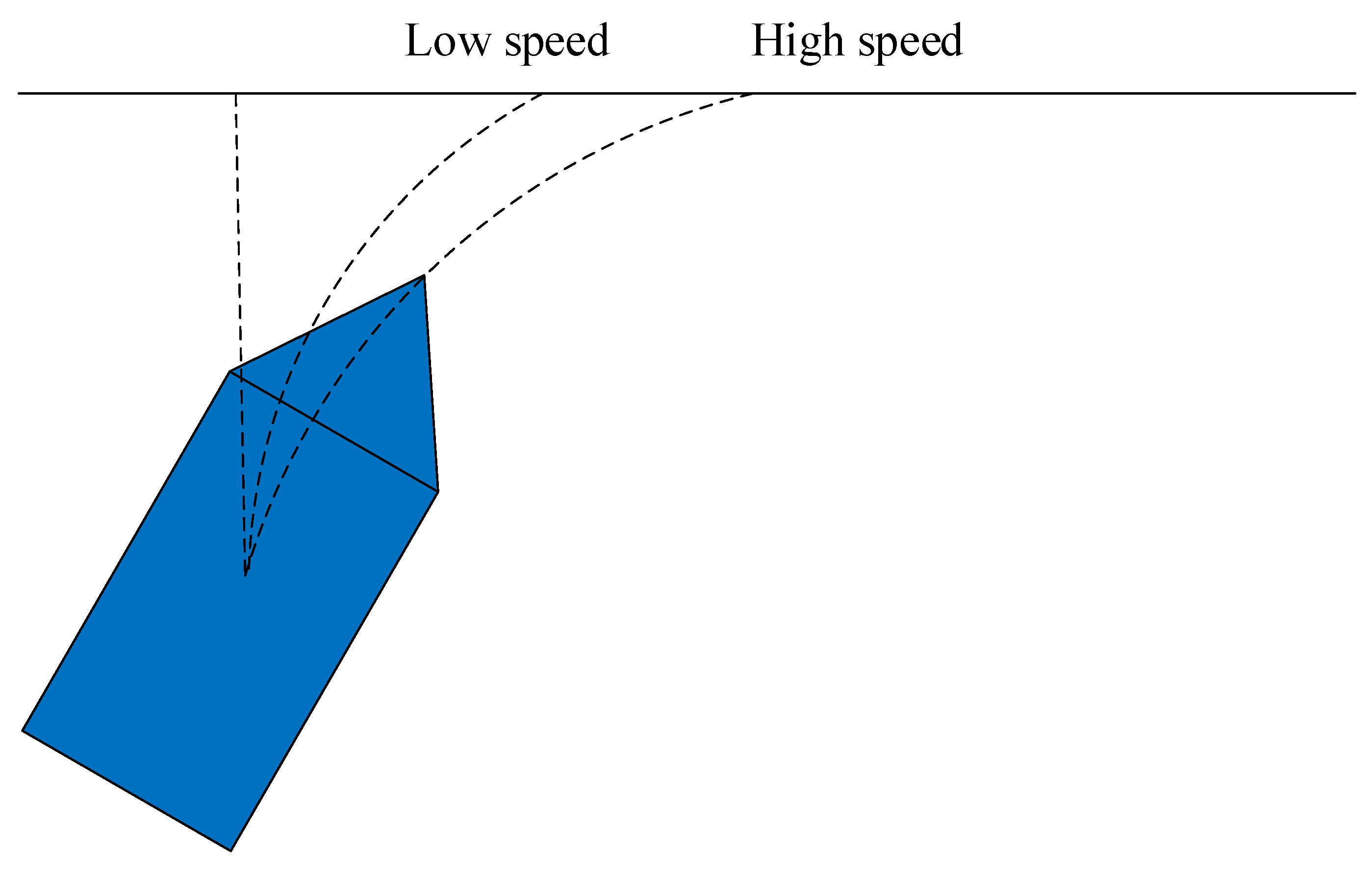
- The look-ahead distance varies with USV speed and tracking error;
- The sideslip angle was estimated online and compensated by the reduced-order state observer;
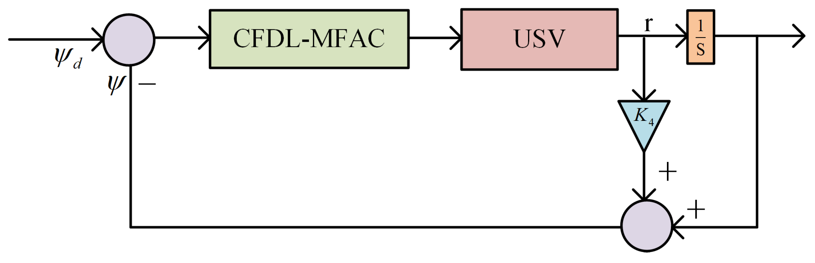
- CFDL-MFAC was designed as a heading controller.
2. Kinematics and Dynamic USV Model
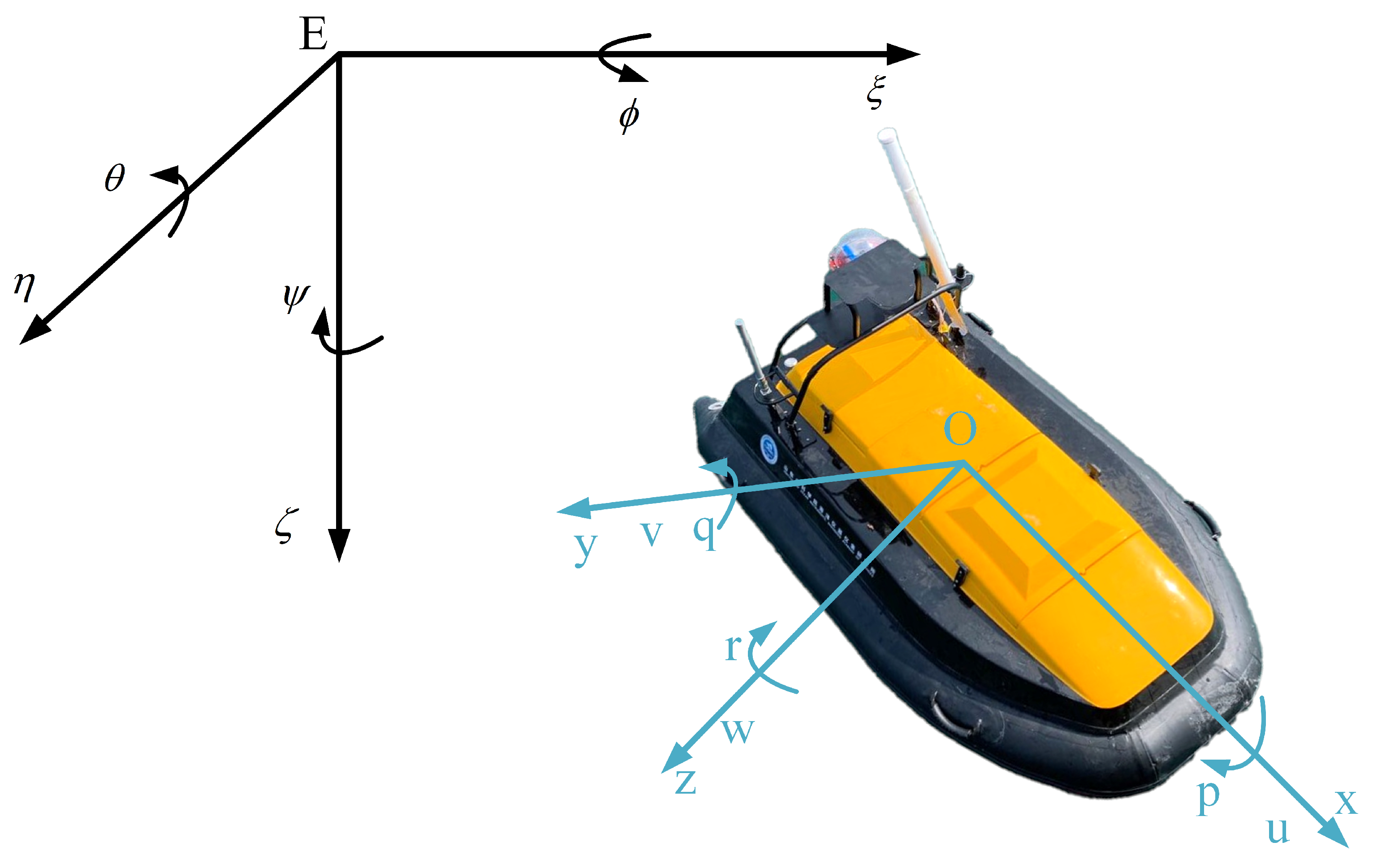
2.1. The Coordinate System Setup
2.2. 3-DOF Model of the USV
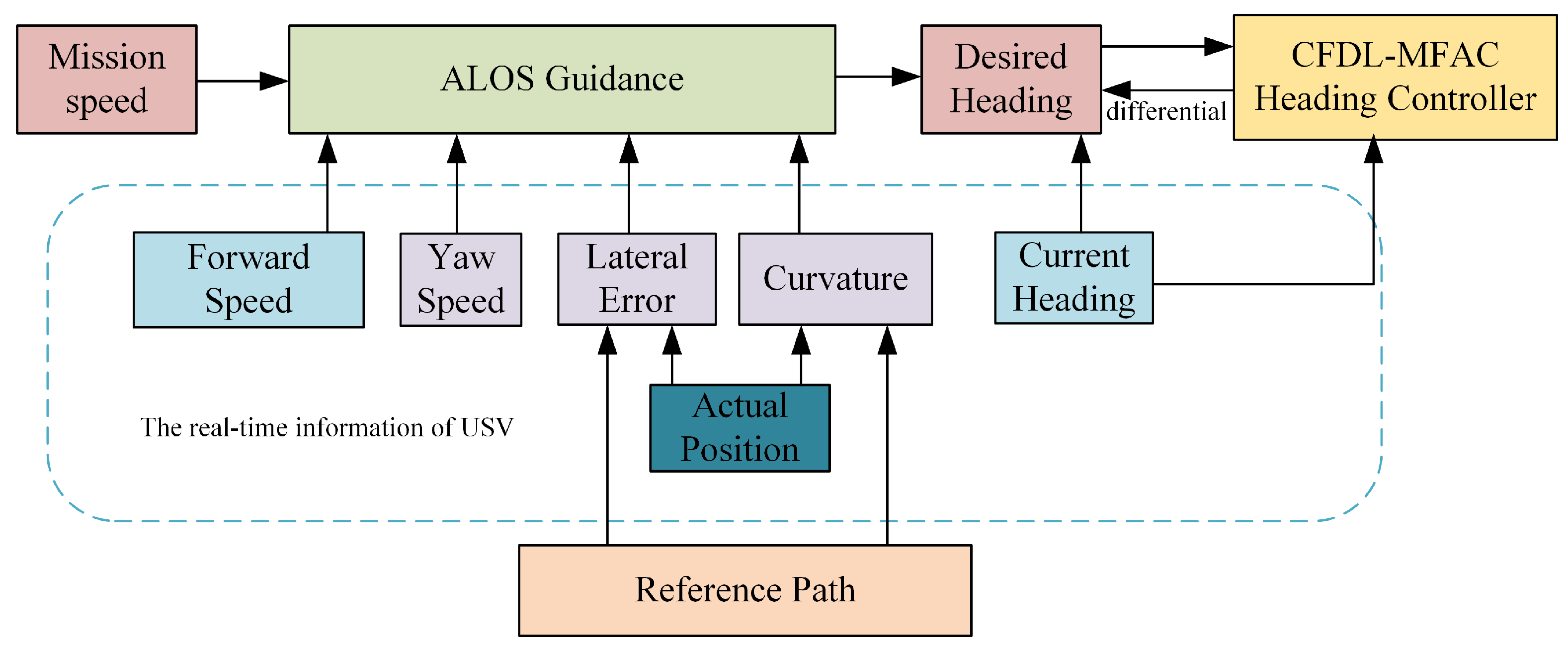
3. Adaptive LOS Guidance Design and Analysis
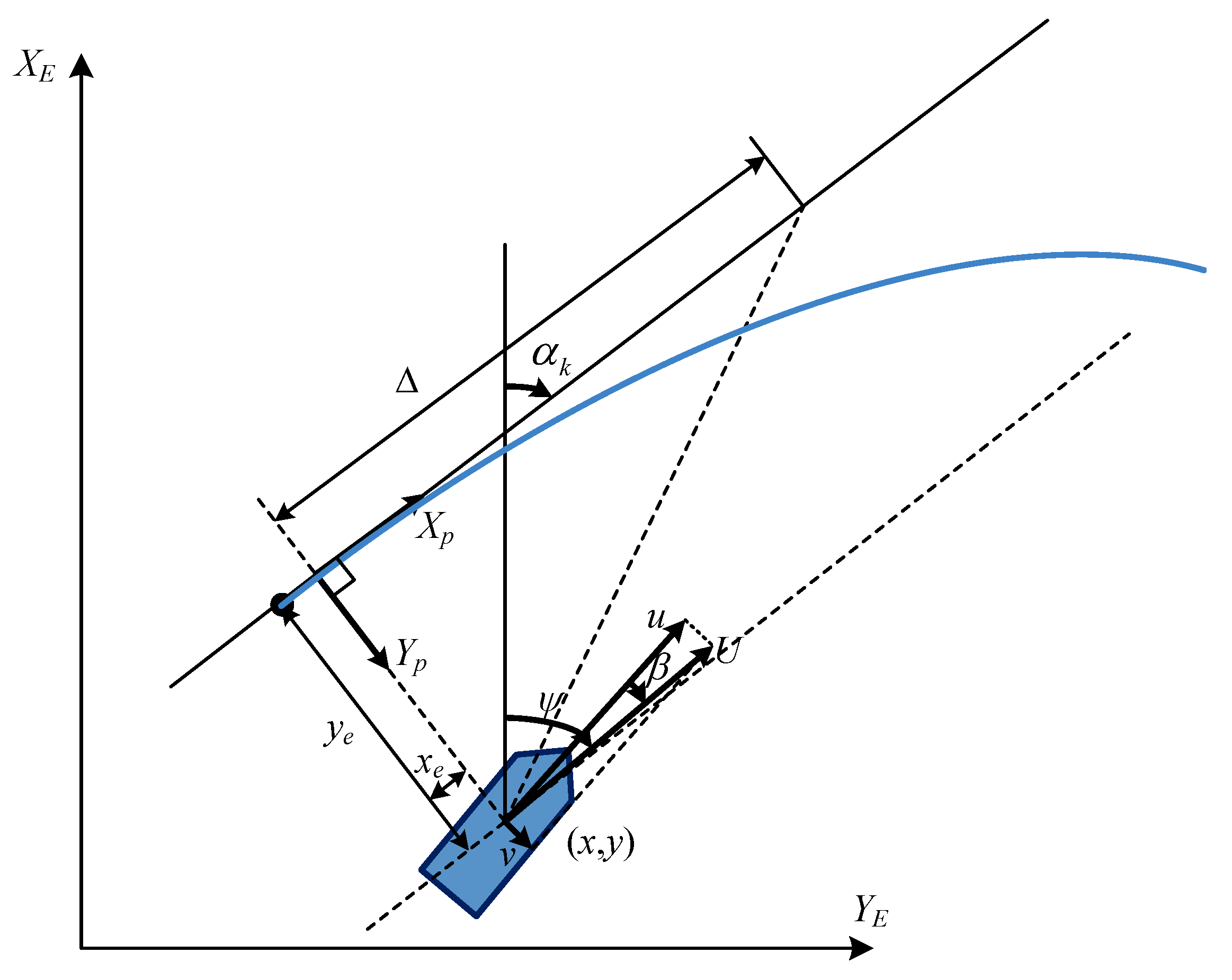
3.1. Path Error Design
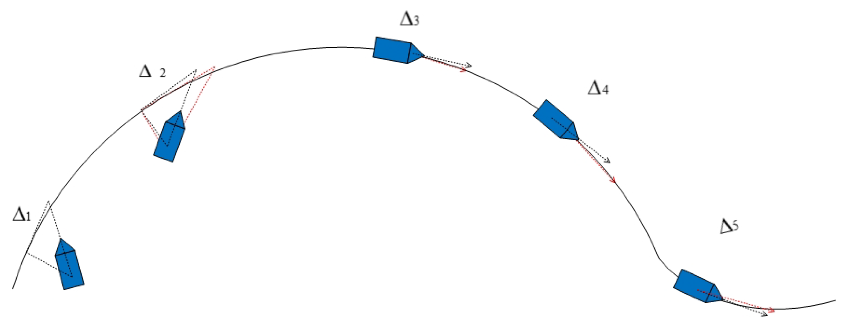
3.2. The Calculation of Look-Ahead Distance
3.3. Reduced-Order State Observer Design
3.4. Guidance Law Design
3.5. Controller Design
4. Simulation
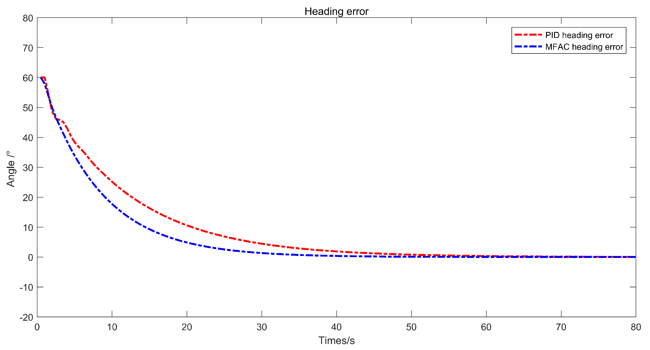
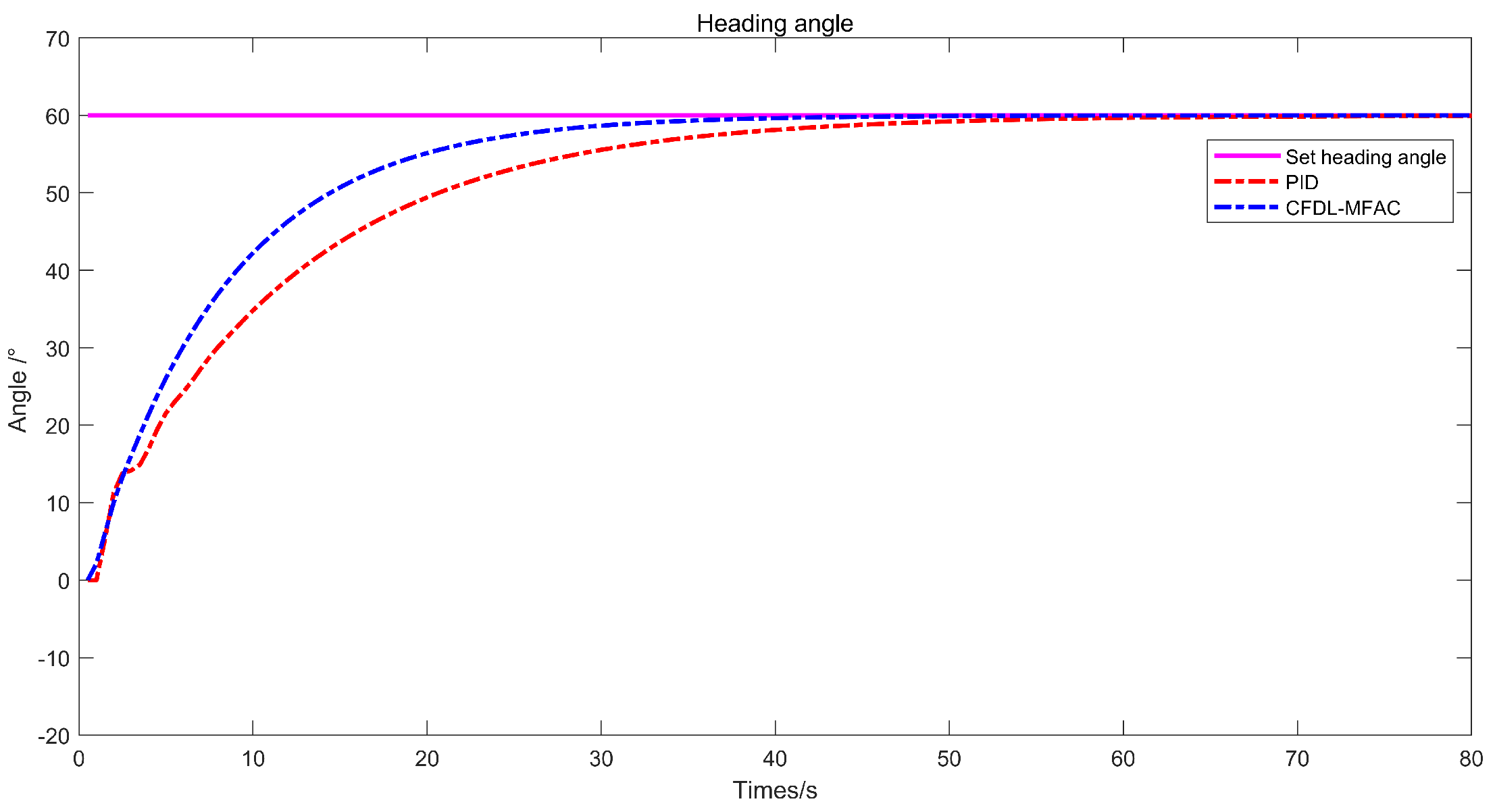
4.1. Heading Control Comparisons
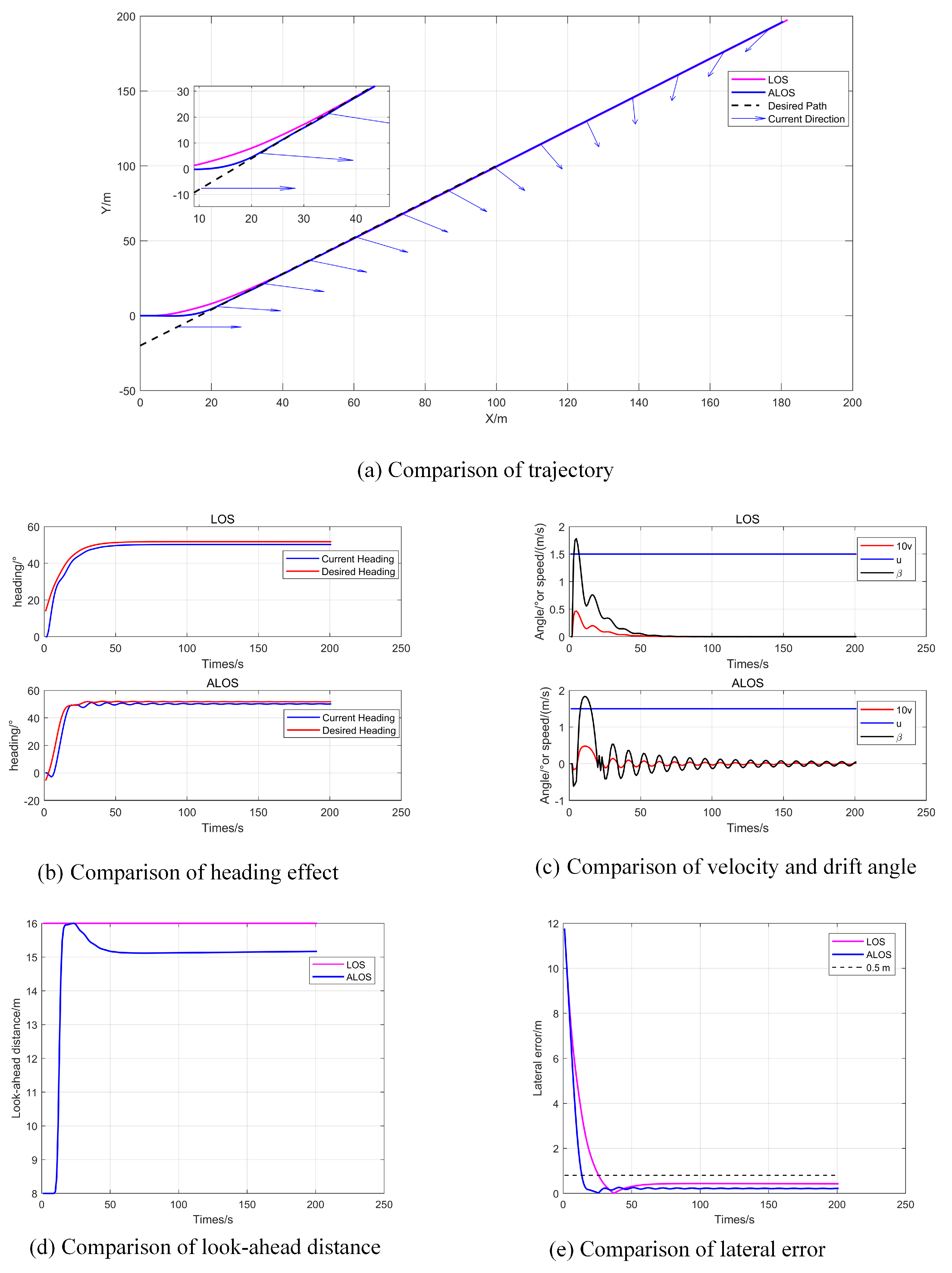
4.2. Tracking Straight-Line Paths in Dynamic Ocean Currents
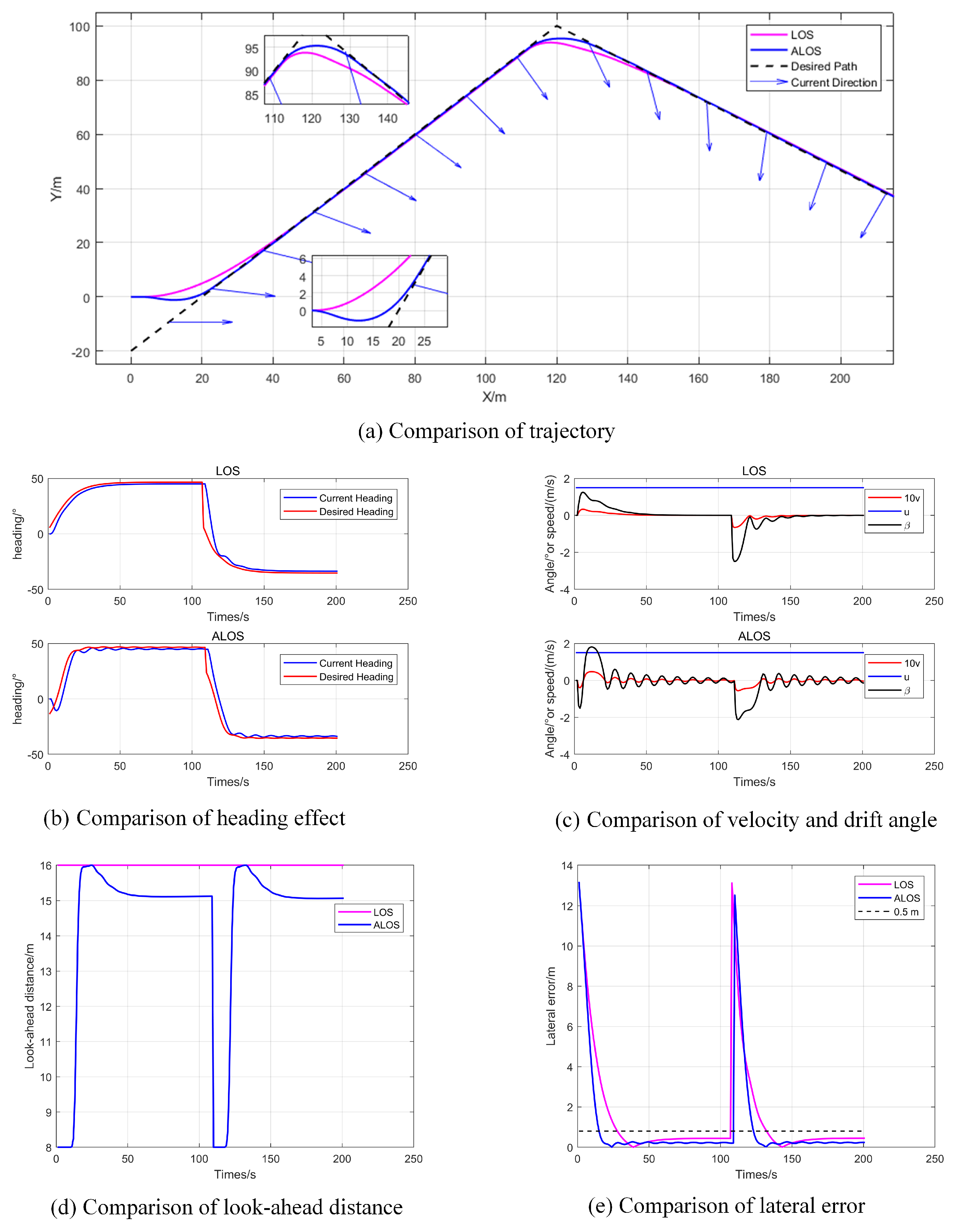
4.3. Folded Line Path Following Under Time-Varying Ocean Current Conditions
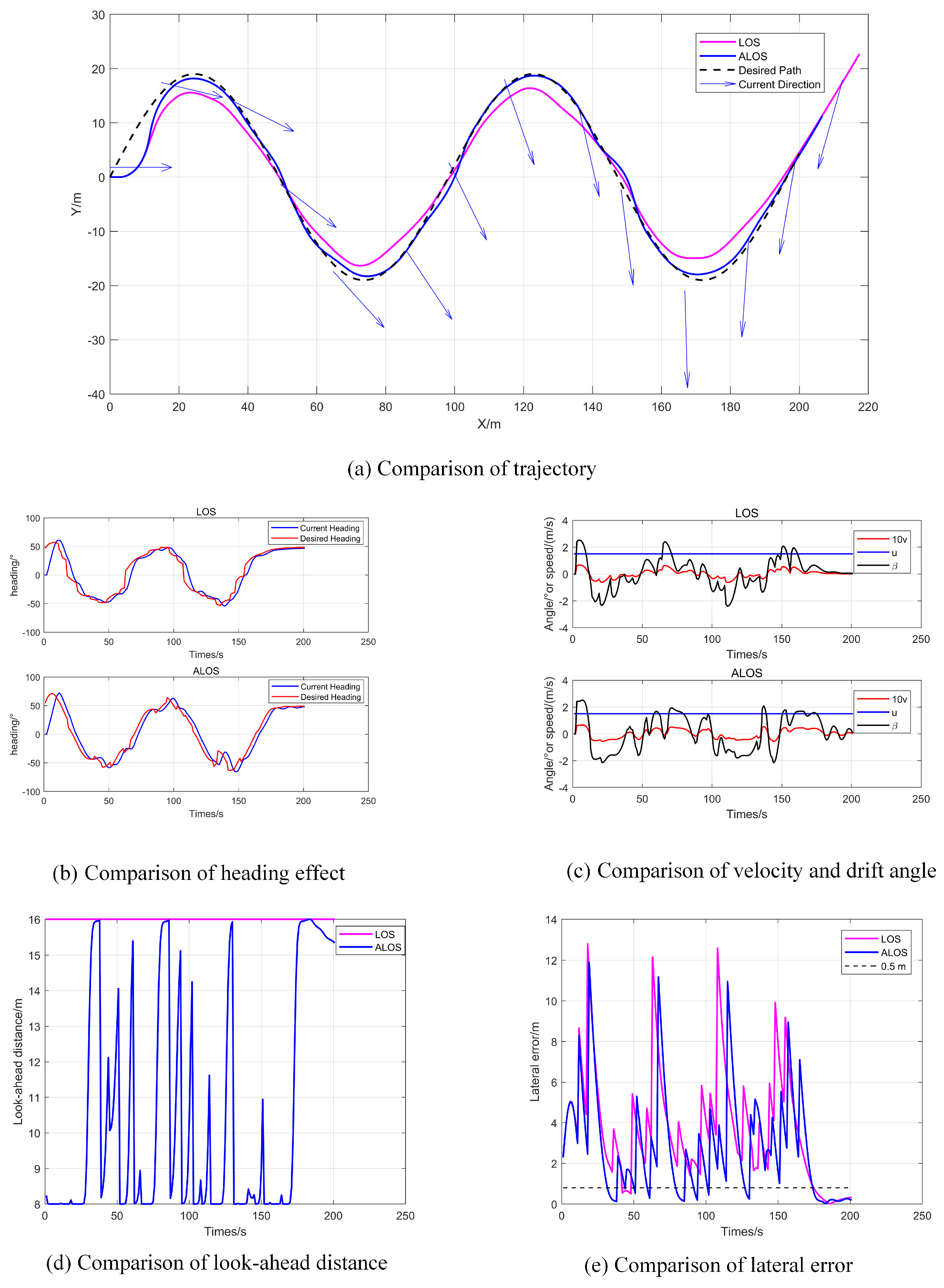
4.4. Sinusoidal Path Following Under Time-Varying Ocean Current Conditions
5. Conclusions
Author Contributions
Funding
Institutional Review Board Statement
Informed Consent Statement
Data Availability Statement
Conflicts of Interest
References
- Liu, Z.; Zhang, Y.; Yu, X.; Yuan, C. Unmanned surface vehicles: An overview of developments and challenges. Annu. Rev. Control 2016, 41, 71–93. [Google Scholar] [CrossRef]
- Shi, B.; Su, Y.; Wang, C.; Wan, L.; Luo, Y. Study on intelligent collision avoidance and recovery path planning system for the waterjet-propelled unmanned surface vehicle. Ocean Eng. 2019, 182, 489–498. [Google Scholar] [CrossRef]
- Wan, L.; Su, Y.; Zhang, H.; Tang, Y.; Shi, B. Global fast terminal sliding mode control based on radial basis function neural network for course keeping of unmanned surface vehicle. Int. J. Adv. Robot. Syst. 2019, 16, 1729881419829961. [Google Scholar] [CrossRef]
- Zhang, G.; Deng, Y.; Zhang, W.; Huang, C. Novel DVS guidance and path-following control for underactuated ships in presence of multiple static and moving obstacles. Ocean Eng. 2018, 170, 100–110. [Google Scholar] [CrossRef]
- Zhang, G.; Deng, Y.; Zhang, W. Robust neural path-following control for underactuated ships with the DVS obstacles avoidance guidance. Ocean Eng. 2017, 143, 198–208. [Google Scholar] [CrossRef]
- Breivik, M.; Fossen, T.I. Guidance Laws for Autonomous Underwater Vehicles; InTech: Takasago, Japan, 2009. [Google Scholar]
- Fossen, T.I. Marine Control System: Guidance, Navigation and Control of Ship, Rigs and Underwater Vehicles. Tapir Trykkeri Trondheim Norway 2002, ch. II, 143–169. [Google Scholar]
- Xiang, X.; Liu, C.; Lapierre, L.; Jouvencel, B. Synchronized Path Following Control of Multiple Homogeneous Underactuated AUVs. J. Syst. Sci. Complex. 2012, 25, 71–89. [Google Scholar] [CrossRef]
- Børhaug, E.; Pavlov, A.; Pettersen, K.Y. Integral LOS control for path following of underactuated marine surface vessels in the presence of constant ocean currents. In Proceedings of the 47th IEEE Conference on Decision and Control, Cancun, Mexico, 9–11 December 2008; pp. 4984–4991. [Google Scholar]
- Fossen, T.I.; Lekkas, A.M. Direct and indirect adaptive integral line-of-sight path-following controllers for marine craft exposed to ocean currents. Int. J. Adapt. Control. Signal Process. 2017, 31, 445–463. [Google Scholar] [CrossRef]
- Encamacao, P.; Pacoal, A.; Arcak, M. Path following for autonomous marine craft. In Proceedings of the 5th IFAC Conference on Manoeuvring and Control of Marine Caraft, Aalborg, Denmark, 23–25 August 2000; pp. 117–122. [Google Scholar]
- Do, K.D.; Jiang, Z.P.; Pan, J. Robust adaptive path following of underactuated ships. Automatica 2004, 40, 929–944. [Google Scholar] [CrossRef]
- Zeng, J.F.; Wan, L.; Li, Y.M.; Zhang, Y.H.; Zhang, Z.Y.; Chen, G.F. Switching-line-of-sight-guidance-based Robust Adaptive Path-following Control for Underactuated Unmanned Surface Vehicles. Acta Armamentarii 2018, 39, 2427–2437. [Google Scholar]
- Zhou, W.; Chang, X.; Zhou, P.; Wang, Y.; Duan, D. Path following control for an under-actuated autonomous airship in constant wind field. In Proceedings of the 2017 29th Chinese Control And Decision Conference (CCDC), Chongqing, China, 28–30 May 2017; pp. 382–387. [Google Scholar]
- Wang, N.; Sun, Z.; Yin, J.; Zou, Z.; Su, S.F. Fuzzy unknown observer-based robust adaptive path following control of underactuated surface vehicles subject to multiple unknowns. Ocean Eng. 2019, 176, 57–64. [Google Scholar] [CrossRef]
- Niu, G.; Wan, L. Model-free Path Following Control of Unmanned Surface Vehicle Based on Adaptive Line-of-sight Guidance. In IOP Conference Series: Earth and Environmental Science; IOP Publishing: Bristol, UK, 2021; Volume 632, p. 032046. [Google Scholar]
- Cheng, S.; Quilodrán-Casas, C.; Ouala, S.; Farchi, A.; Liu, C.; Tandeo, P.; Fablet, R.; Lucor, D.; Iooss, B.; Brajard, J.; et al. Machine learning with data assimilation and uncertainty quantification for dynamical systems: A review. J. Comput. Phys. 2021, 426, 109935. [Google Scholar] [CrossRef]
- Bos, J.T.O.; Dijkstra, H.A.; van Leeuwen, P.J. Model-reduced variational data assimilation. Mon. Weather. Rev. 2008, 136, 3657–3677. [Google Scholar]
- Cheng, S.; Zhuang, Y.; Kahouadji, L.; Liu, C.; Chen, J.; Matar, O.K.; Arcucci, R. Multi-domain encoder-decoder neural networks for latent data assimilation in dynamical systems. Phys. Fluids 2022, 34, 056606. [Google Scholar] [CrossRef]
- Zhang, G.; Li, J.; Chang, T.; Zhang, W.; Song, L. Autonomous navigation and control for a sustainable vessel: A wind-assisted strategy. Sustain. Horizons 2025, 2, 10–20. [Google Scholar] [CrossRef]
- Zhang, G.; Yin, S.; Huang, C.; Zhang, W.; Li, J. Structure Synchronized Dynamic Event-Triggered Control for Marine Ranching AMVs via the Multi-Task Switching Guidance. IEEE Trans. Intell. Transp. Syst. 2024, 25, 1234–1246. [Google Scholar] [CrossRef]
- Wang, Y.; Tong, H.; Fu, M. Line-of-sight guidance law for path following of amphibious hovercrafts with big and time-varying sideslip compensation. Ocean Eng. 2019, 172, 531–540. [Google Scholar] [CrossRef]
- Li, M.; Guo, C.; Yu, H. Filtered Extended State Observer based Line-of-Sight Guidance for Path Following of Unmanned Surface Vehicles with Unknown Dynamics and Disturbances. IEEE Access 2019, 7, 178401–178412. [Google Scholar] [CrossRef]
- Wang, D.; He, B.; Shen, Y.; Li, G.; Chen, G. A Modified ALOS Method of Path Tracking for AUVs with Reinforcement Learning Accelerated by Dynamic Data-Driven AUV Model. J. Intell. Robot. Syst. 2022, 103, 49. [Google Scholar] [CrossRef]
- Mu, D.; Wang, G.; Fan, Y. Path Following Control Strategy for Underactuated Unmanned Surface Vehicle Subject to Multiple Constraints. IEEJ Trans. Electr. Electron. Eng. 2022, 17, 229–241. [Google Scholar] [CrossRef]
- Zhao, Y.; Qi, X.; Incecik, A.; Ma, Y.; Li, Z. Broken lines path following algorithm for a water-jet propulsion USV with disturbance uncertainties. Ocean Eng. 2020, 201, 107118. [Google Scholar] [CrossRef]
- Huang, Y.; Shi, X.; Huang, W.; Chen, S. Internal Model Control-Based Observer for the Sideslip Angle of an Unmanned Surface Vehicle. J. Mar. Sci. Eng. 2022, 10, 470. [Google Scholar] [CrossRef]
- Mobarez, E.N.; Mobariz, K.N.; Ashry, M.M. Marine Control System Design Based on Different PID Approaches. In Proceedings of the 2021 Tenth International Conference on Intelligent Computing and Information Systems (ICICIS), Cairo, Egypt, 5–7 December 2021; pp. 254–257. [Google Scholar]
- Gonzalez-Garcia, A.; Castañeda, H. Guidance and Control Based on Adaptive Sliding Mode Strategy for a USV Subject to Uncertainties. IEEE J. Ocean. Eng. 2021, 46, 1144–1154. [Google Scholar] [CrossRef]
- Liu, L.; Li, Z.; Chen, Y.; Wang, R. Disturbance Observer-Based Adaptive Intelligent Control of Marine Vessel With Position and Heading Constraint Condition Related to Desired Output. IEEE Trans. Neural Networks Learn. Syst. 2024, 35, 5870–5879. [Google Scholar] [CrossRef]
- Liu, Z.; Xiang, Q.; Ye, X.; Yu, L. Unmanned Surface Vehicle Heading and Speed Control Method Based on Model Predictive Control. In Proceedings of the 2022 IEEE 5th International Conference on Electronics Technology (ICET), Chengdu, China, 13–16 May 2022; pp. 612–616. [Google Scholar]
- Hou, Z.; Huang, W. The model-free learning adaptive control of a class of nonlinear discrete-time systems. IFAC Proc. Vol. 1998, 15, 893–899. [Google Scholar] [CrossRef]
- Hou, Z. Model Free Adaptive Control: Theory and Applications; Springer: Berlin/Heidelberg, Germany, 2013. [Google Scholar]
- Hou, Z.; Liu, S.; Tian, T. Lazy-Learning-Based Data-Driven Model-Free Adaptive Predictive Control for a Class of Discrete-Time Nonlinear Systems. IEEE Trans. Neural Networks Learn. Syst. 2017, 28, 1914–1928. [Google Scholar] [CrossRef]
- Liu, F.; Shen, Y.; He, B.; Wan, J.; Wang, D.; Yin, Q.; Qin, P. 3DOF Adaptive Line-Of-Sight Based Proportional Guidance Law for Path Following of AUV in the Presence of Ocean Currents. Appl. Sci. 2019, 9, 3518. [Google Scholar] [CrossRef]
- Liu, F.; Shen, Y.; He, B.; Wang, D.; Wan, J.; Sha, Q.; Qin, P. Drift angle compensation-based adaptive line-of-sight path following for autonomous underwater vehicle. Appl. Ocean. Res. 2019, 93, 101943. [Google Scholar] [CrossRef]
- Fossen, T.I. Handbook of Marine Craft Hydrodynamics and Motion Control; John Willy & Sons Ltd.: Hoboken, NJ, USA, 2011. [Google Scholar]
- Khalil, H.K. Nonlinear Systems. Automatica 2002, 38, 1091–1093. [Google Scholar] [CrossRef]

| Vector | X-Axis | Y-Axis | Z-Axis |
|---|---|---|---|
| Euler Angle | |||
| Linear Velocity | u | v | w |
| Angle Velocity | p | q | r |
| Displacement | x | y | z |
| Parameters | Value | Units |
|---|---|---|
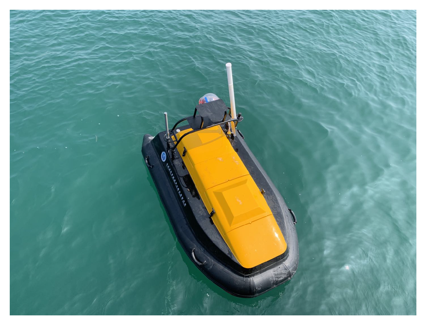
| Length | 194 | cm |
| Width | 110 | cm |
| Weight | 56 | Kg |
| Maximum Power | 1200 | W |
| Name | LOS | ALOS | Improvement |
|---|---|---|---|
| MAE (m) | 0.9253 | 0.5760 | |
| RMSE (m) | 2.0121 | 1.7397 |
| Name | LOS | ALOS | Improvement |
|---|---|---|---|
| MAE(m) | 1.0420 | ||
| RMSE(m) | 3.1100 | 6 |
| LOS | ALOS | Improvement | |
|---|---|---|---|
| MAE (m) | 3.7429 | 2.8647 | |
| RMSE (m) | 4.6752 | 3.8550 |
Disclaimer/Publisher’s Note: The statements, opinions and data contained in all publications are solely those of the individual author(s) and contributor(s) and not of MDPI and/or the editor(s). MDPI and/or the editor(s) disclaim responsibility for any injury to people or property resulting from any ideas, methods, instructions or products referred to in the content. |
© 2025 by the authors. Licensee MDPI, Basel, Switzerland. This article is an open access article distributed under the terms and conditions of the Creative Commons Attribution (CC BY) license (https://creativecommons.org/licenses/by/4.0/).
Share and Cite
Li, Y.; Wan, J.; Wang, X.; Sun, Z.; Li, H.; Yu, Z.; Kou, L.; Li, J.; Yang, Y. Path-Following Control Based on ALOS Guidance Law for USV. Electronics 2025, 14, 749. https://doi.org/10.3390/electronics14040749
Li Y, Wan J, Wang X, Sun Z, Li H, Yu Z, Kou L, Li J, Yang Y. Path-Following Control Based on ALOS Guidance Law for USV. Electronics. 2025; 14(4):749. https://doi.org/10.3390/electronics14040749
Chicago/Turabian StyleLi, Yanping, Junhe Wan, Xiaolei Wang, Zeqiang Sun, Hui Li, Zhen Yu, Lei Kou, Junxiao Li, and Yang Yang. 2025. "Path-Following Control Based on ALOS Guidance Law for USV" Electronics 14, no. 4: 749. https://doi.org/10.3390/electronics14040749
APA StyleLi, Y., Wan, J., Wang, X., Sun, Z., Li, H., Yu, Z., Kou, L., Li, J., & Yang, Y. (2025). Path-Following Control Based on ALOS Guidance Law for USV. Electronics, 14(4), 749. https://doi.org/10.3390/electronics14040749