
Pole-to-Pole Fault Current Impact Factors Analysis Based on Equivalent Impedance for Modular Multilevel Converter High-Voltage Direct Current System

Abstract
1. Introduction
2. MMC Circuit and Model in Different Control Modes
2.1. Equivalent Circuit for Converter
2.2. The Modeling of the AC System and the Inner Control Loop
2.3. The Modeling of the Outer Control Loop in Different Modes
- ■
- Constant power control mode
- ■
- Constant DC voltage control mode
- ■
- Droop control
3. The MMC Equivalent Impedance Model for Fault Current Analysis
3.1. MMC Detailed Equivalent Impedance Model
3.2. The Simplified MMC Equivalent Impedance Model for Fault Current Analysis
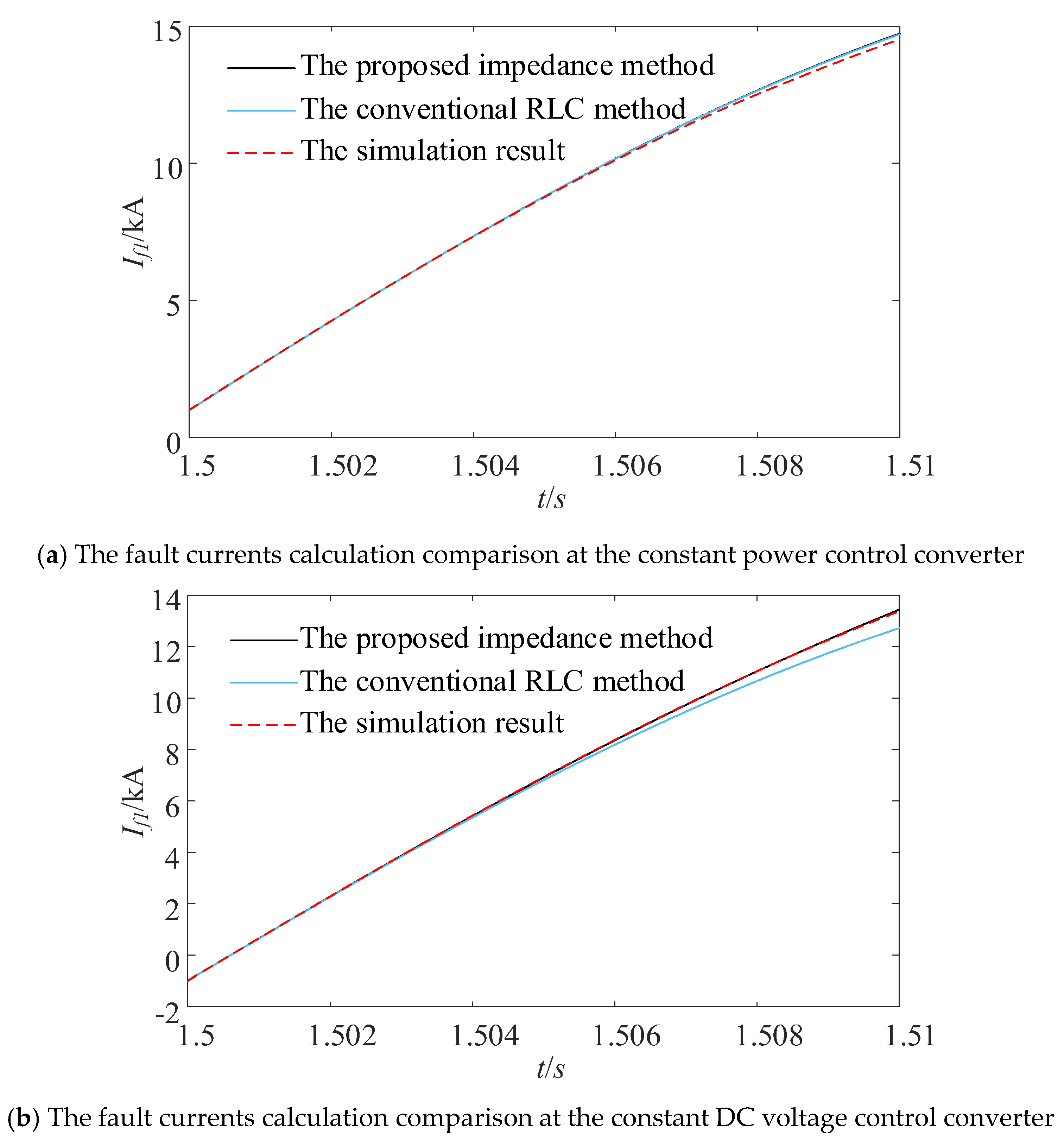
3.3. The Fault Current Calculation Method Based on MMC Equivalent Model
4. The Fault Current Impact Factor Analysis Based on Impedance Calculation
4.1. The Device Parameters’ Impact on Equivalent Impedance
- ■
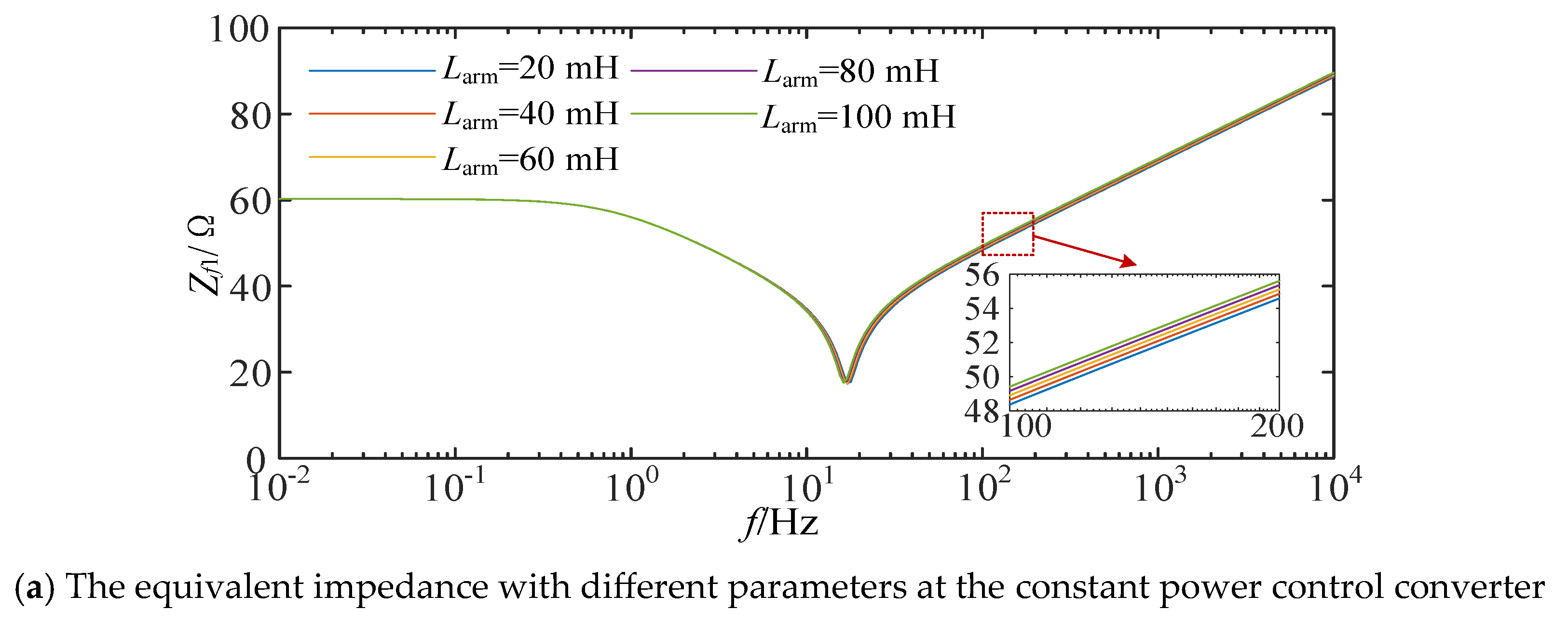
- The arm inductance’s impact on equivalent impedance
- ■
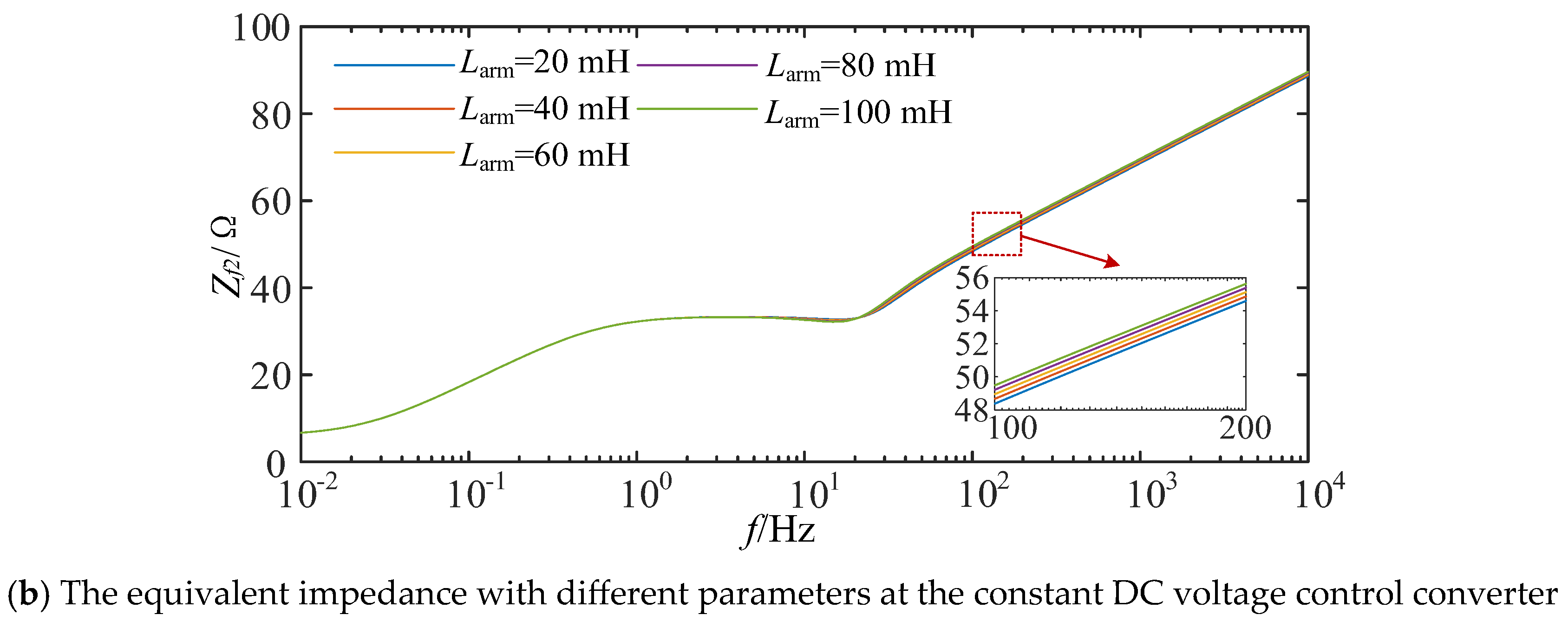
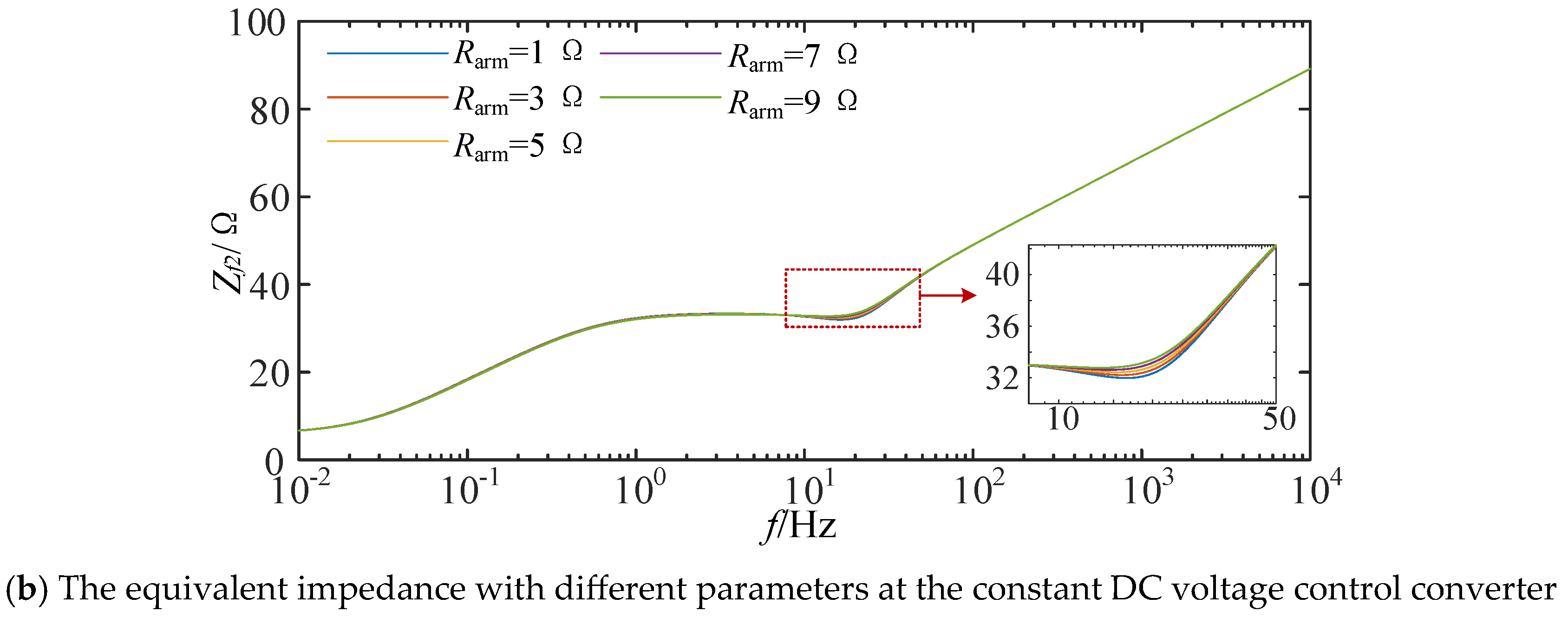
- The arm resistance’s impact on equivalent impedance.
- ■
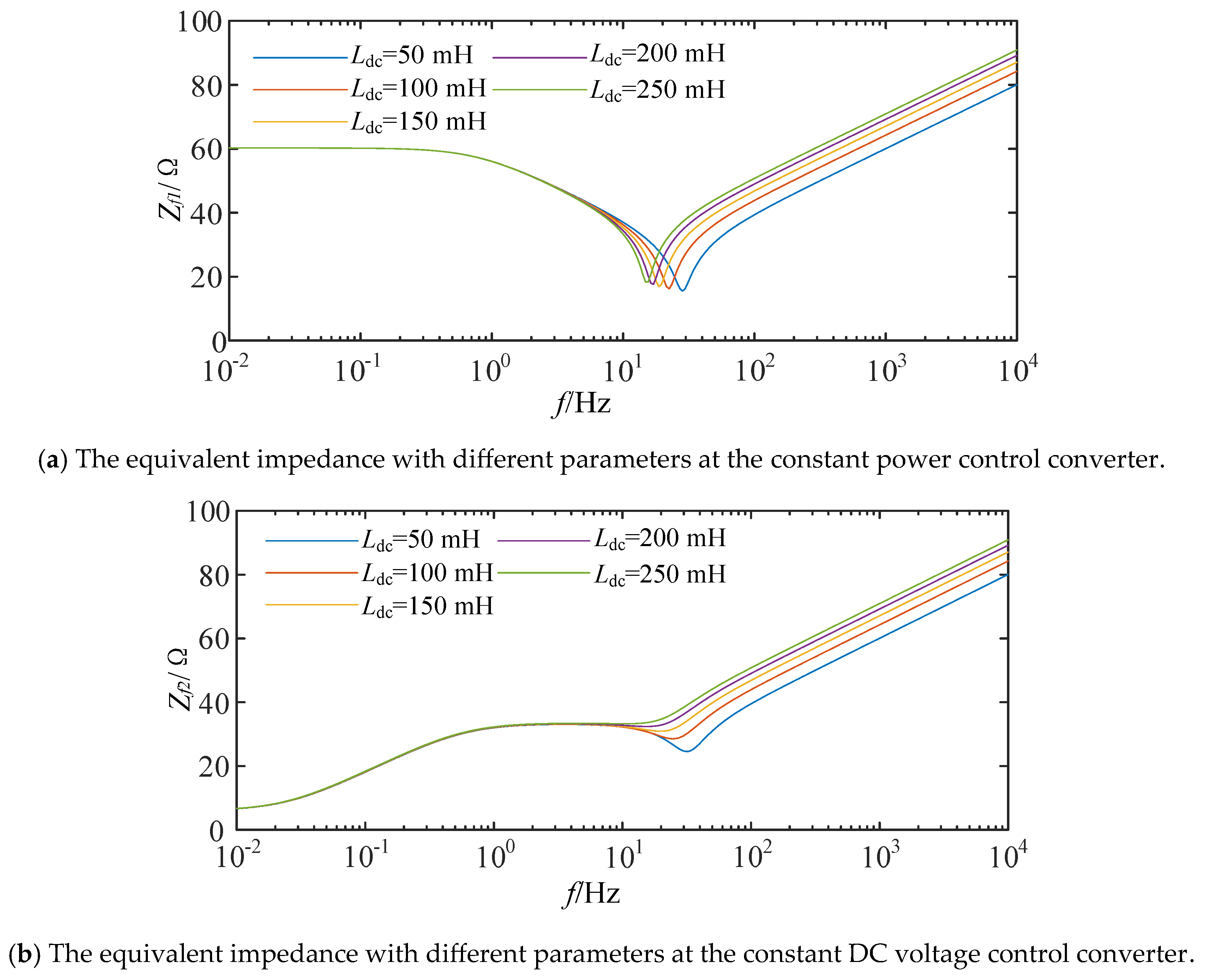
- The smoothing reactor’s impact on equivalent impedance.
- ■
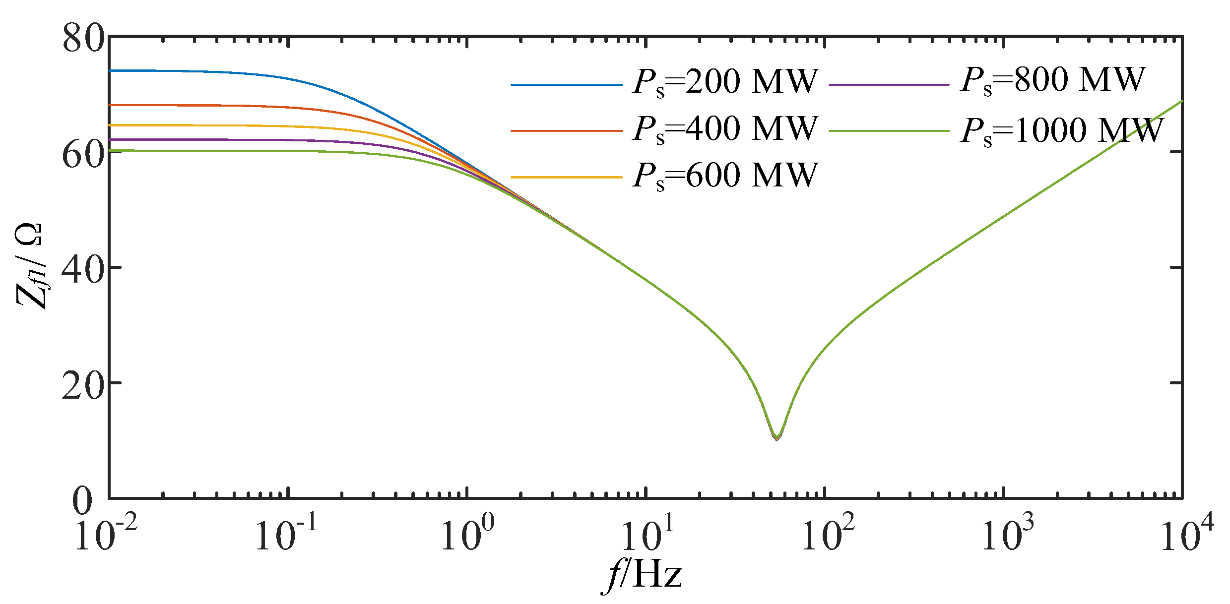
- Power control’s impact on equivalent impedance.
4.2. The Device Parameters’ Impact on Fault Current
- ■
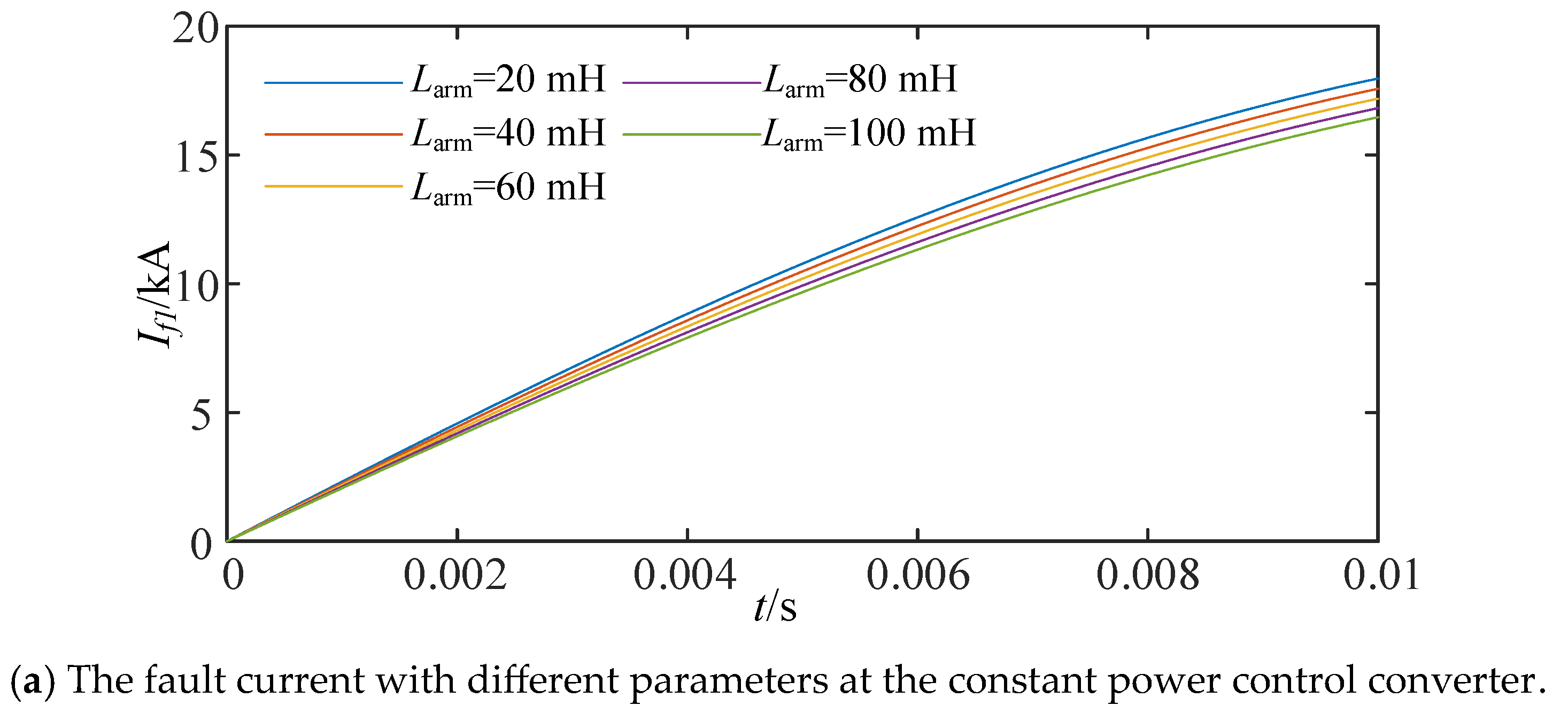
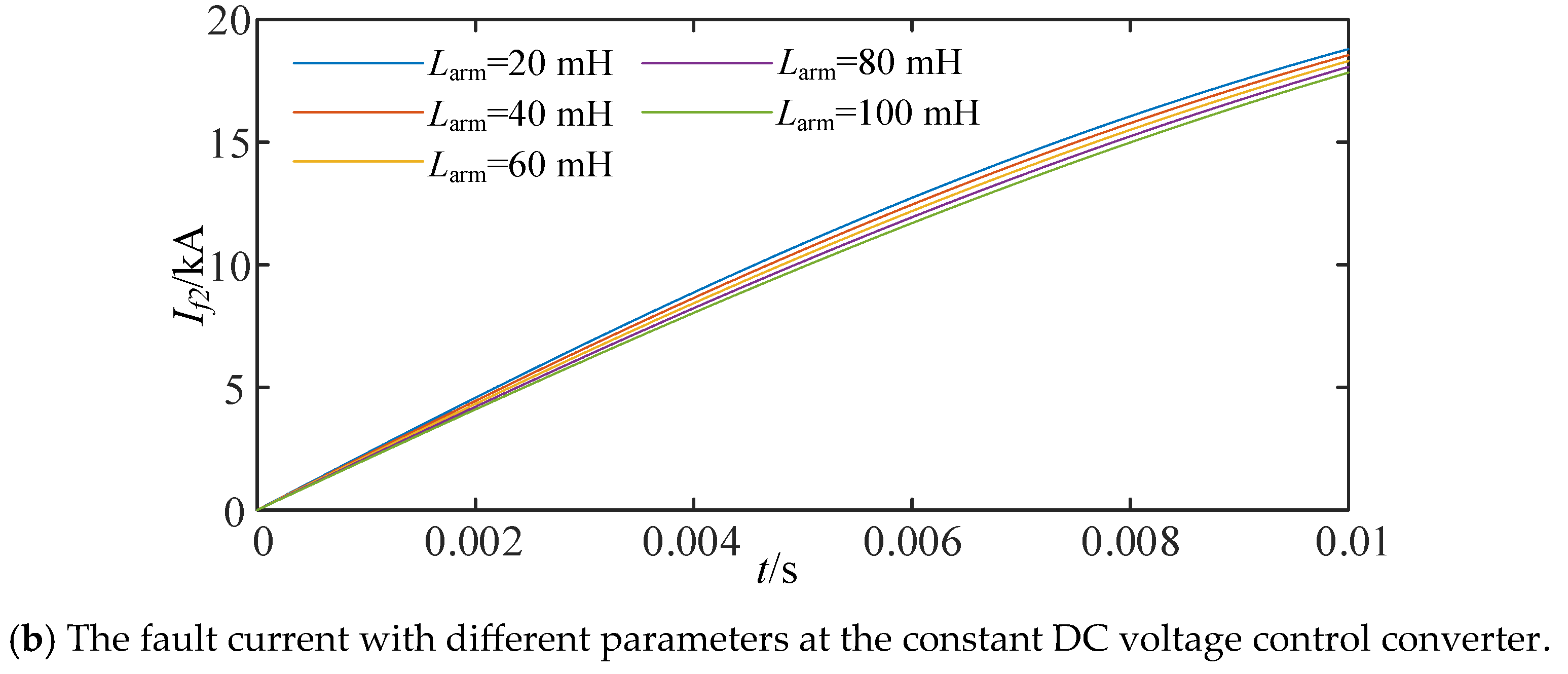
- The arm inductance’s impact on fault current.
- ■
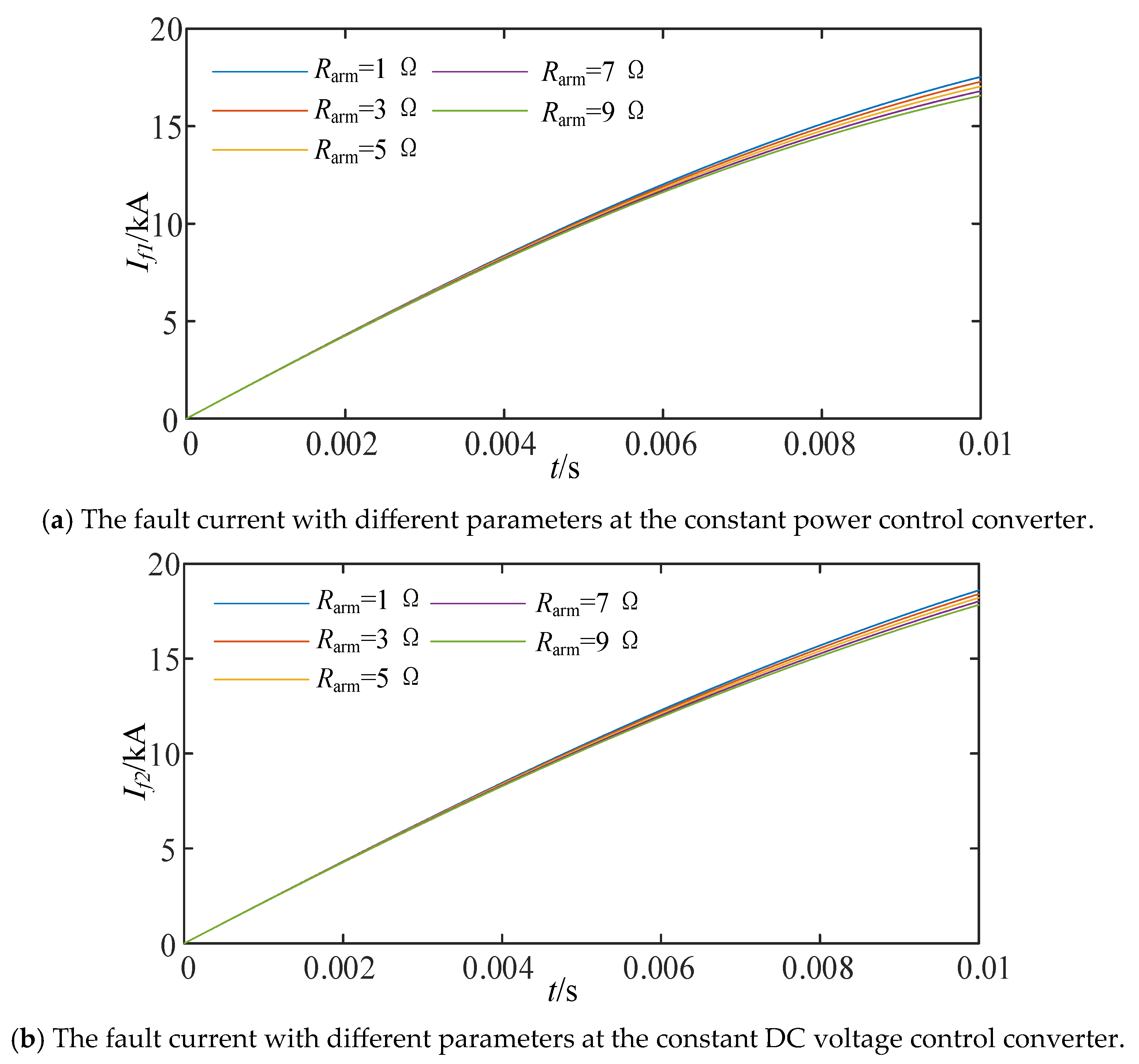
- The arm resistance’s impact on fault current
- ■
- The smoothing reactor’s impact on fault current.
- ■
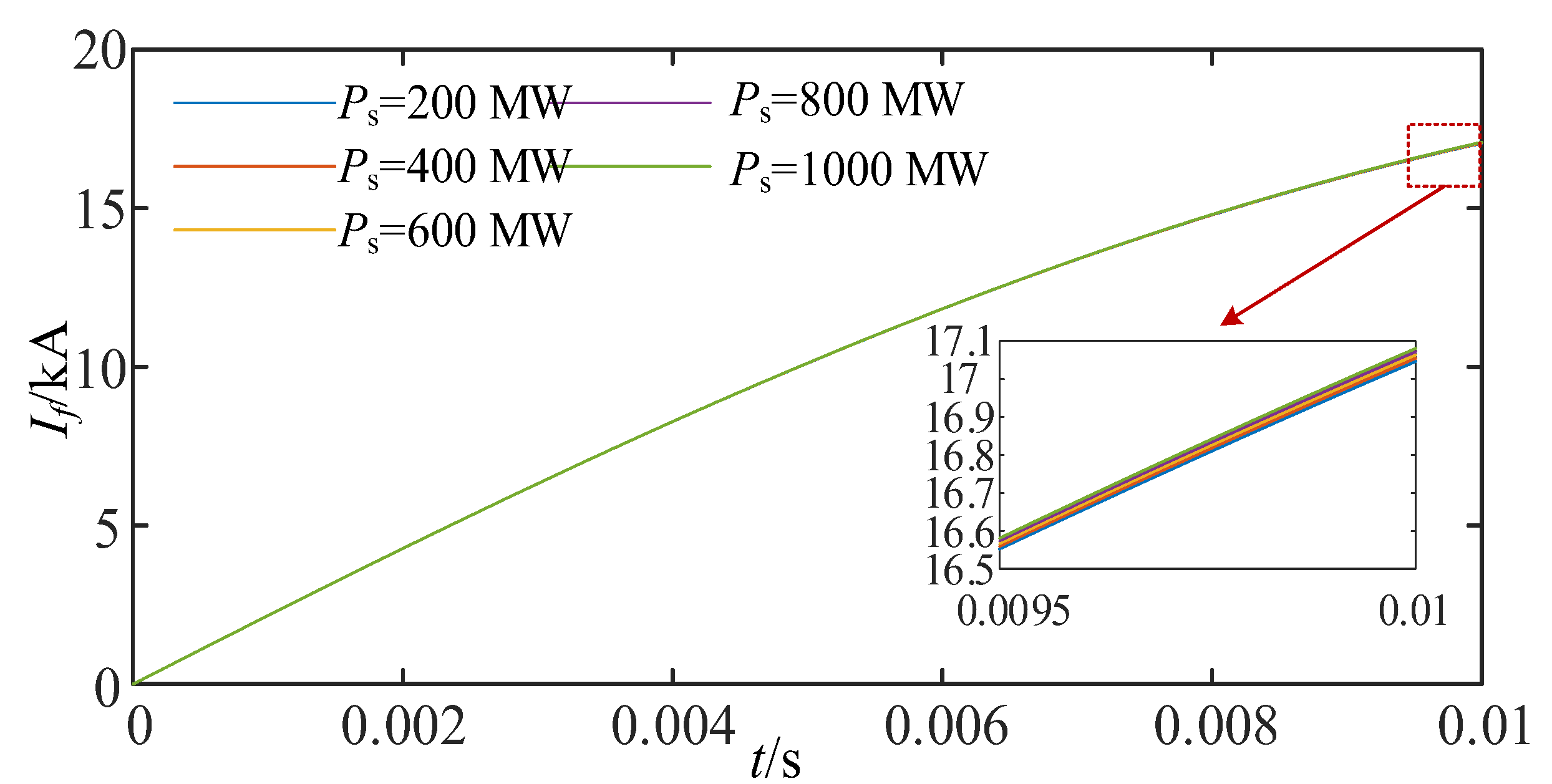
- Power control’s impact on equivalent impedance.
5. Conclusions
- (1)
- The low-frequency component of the equivalent impedance has no significant impact on the rate of increase and the peak value of the fault current during the initial stage (typically referring to the first 10 ms after the fault occurs), such as the DC power level. The mid-frequency component of the equivalent impedance does not affect the initial rate of increase in the fault current, but it does influence the current level several milliseconds after the fault occurs. Factors such as arm resistance and submodule capacitance, when their values change, will lead to variations in the fault current.
- (2)
- The high-frequency component of fault damping primarily influences the initial state of the fault current, specifically the initial rate of increase. Components such as the smoothing reactor, when their values change, can significantly alter the initial rate of increase in the fault current, thereby affecting the subsequent current levels. The damping characteristics in the high-frequency range have the most pronounced impact on the fault current.
Author Contributions
Funding
Data Availability Statement
Conflicts of Interest
References
- Tao, Y.; Li, B.; Dragicevic, T.; Liu, T.; Blaabjerg, F. HVDC Grid Fault Current Limiting Method Through Topology Optimization Based on Genetic Algorithm. IEEE J. Emerg. Sel. Top. Power Electron. 2021, 9, 7045–7055. [Google Scholar] [CrossRef]
- Ouyang, J.; Yu, J.; Long, X.; Diao, Y.; Wang, J. Coordination control method to block cascading failure of a renewable generation power system under line dynamic security. Prot. Control. Mod. Power Syst. 2023, 8, 12. [Google Scholar] [CrossRef]
- Yang, Z.; Wang, H.; Liao, W.; Bak, C.L.; Chen, Z. Protection Challenges and Solutions for AC Systems with Renewable Energy Sources: A Review. Prot. Control. Mod. Power Syst. 2024, 10, 18–39. [Google Scholar] [CrossRef]
- Tao, Y.; Li, B.; Liu, T.; Jiang, Q.; Blaabjerg, F. Practical Fault Current Level Evaluation and Limiting Method of Bipolar HVdc Grid Based on Topology Optimization. IEEE Syst. J. 2022, 16, 4466–4476. [Google Scholar] [CrossRef]
- Jiang, Q.; Xu, R.; Li, B.; Chen, X.; Yin, Y.; Liu, T. Impedance Model for Instability Analysis of LCC-HVDCs Considering Transformer Saturation. J. Mod. Power Syst. Clean Energy 2024, 12, 1309–1319. [Google Scholar] [CrossRef]
- Zhou, H.; Li, B.; Jiang, Q.; Liu, T.; Zhang, Y.; Yin, Y. The Extreme Temperature Weather Impact Mechanism Analysis of MMC-HVDC’s Harmonic Impedance and Its Dynamic Stability. Energies 2024, 17, 6044. [Google Scholar] [CrossRef]
- Han, X.; Sima, W.; Yang, M.; Li, L.; Yuan, T.; Si, Y. Transient Characteristics Under Ground and Short-Circuit Faults in a ±500 kV MMC-Based HVDC System with Hybrid DC Circuit Breakers. IEEE Trans. Power Deliv. 2018, 33, 1378–1387. [Google Scholar] [CrossRef]
- Bucher, M.K.; Franck, C.M. Contribution of fault current sources in multiterminal HVDC cable networks. IEEE Trans. Power Deliv. 2013, 28, 1796–1803. [Google Scholar] [CrossRef]
- Jianpo, Z.; Chengyong, Z. Simulation and analysis of DC-link fault characteristics for MMCHVDC. Electr. Power Autom. Equip. 2014, 34, 32–37. [Google Scholar]
- Zhang, X.; Zhao, C.; Pang, H.; Lin, C. A control and protection scheme of multi-terminal DC transmission system based on MMC for DC line fault. Autom. Electr. Power Syst. 2013, 37, 140–145. [Google Scholar] [CrossRef]
- Ziguang, Z.; Yuan, F.; Yi, W. Pole-to-ground fault analysis of transmission lines in VSC based DC power grids. Mod. Electr. Power 2017, 34, 82–88. [Google Scholar]
- Jovcic, D.; Pahalawaththa, N.; Zavahir, M. Inverter controller for HVDC systems connected to weak AC systems. IEEE Proc. Gener. Transm. Distrib. 1999, 146, 235–240. [Google Scholar] [CrossRef]
- Wang, S.; Zhou, X.; Tang, G. Analysis of submodule overcurrent caused by DC pole-to-pole fault in modular multilevel converter HVDC system. Proc. CSEE 2011, 31, 1–7. [Google Scholar]
- Li, C.; Zhao, C.; Xu, J.; Ji, Y.; Zhang, F.; An, T. A pole-to-pole short-circuit fault current calculation method for DC grids. IEEE Trans. Power Syst. 2017, 32, 4943–4953. [Google Scholar] [CrossRef]
- Ning, C.; Lei, Q.; Xiang, C. Calculation method for line-to-ground short-circuit currents of VSC-HVDC grid. Electr. Power Constr. 2019, 40, 119–127. [Google Scholar]
- Hao, L.; Li, W.; Wang, Z.; Gu, Y.; Wang, G. Practical calculation for bipolar short-circuit fault current of transmission line in MMC-HVDC grid. Autom. Electr. Power Syst. 2020, 44, 68–76. [Google Scholar]
- Yao, L.Z.; Yao, Z.Q.; Lin, Z. DC fault characteristics of modular multilevel converter based HVDC transformer. Power Energy Soc. Gen. Meet. 2011, 40, 1051–1058. [Google Scholar]
- Lacerda, V.A.; Monaro, R.M.; Campos-Gaona, D.; Peña-Alzola, R.; Coury, D.V. An approximated analytical model for pole-to-ground faults in symmetrical monopole MMC-HVDC systems. IEEE J. Emerg. Sel. Top. Power Electron. 2021, 9, 7009–7017. [Google Scholar] [CrossRef]
- Leterme, W.; Tielens, P.; De Boeck, S.; Van Hertem, D. Overview of grounding and configuration options for meshed HVDC grids. IEEE Trans. Power Del. 2014, 29, 2467–2475. [Google Scholar] [CrossRef]
- Yan, L.I.; Huang, Y.; Yanfeng, G. Analysis on overvoltage mechanism of DC line fault in flexible DC grid. Autom. Electr. Power Syst. 2020, 44, 146–153. [Google Scholar]
- Xue, Y.; Zheng, X. On the bipolar MMC-HVDC topology suitable for bulk power overhead line transmission: Configuration, control, and DC fault analysis. IEEE Trans. Power Deliv. 2014, 29, 2420–2429. [Google Scholar] [CrossRef]
- Zhao, C.; Lei, Q.; Chen, N.; Cui, X.; Ma, J. Unipolar ground fault of ±500 kV Zhangbei flexible DC power grid and sound pole bus overvoltage generation mechanism. Power Syst. Technol. 2019, 43, 530–536. [Google Scholar]
- Duan, G.; Wang, Y.; Yin, T.; Yin, S. DC short circuit current calculation for modular multilevel converter. Power Syst. Technol. 2018, 42, 2145–2152. [Google Scholar]
- Li, Q.; Li, B.; Jiang, Q.; Liu, T.; Yue, Y.; Zhang, Y. A Novel Location Method for Interline Power Flow Controllers Based on Entropy Theory. Prot. Control. Mod. Power Syst. 2024, 9, 70–81. [Google Scholar] [CrossRef]


| The Typical Existing Models for DC Fault Current Calculations | Advantages | Disadvantages |
|---|---|---|
| Numerical computation methods | Suitable for different DC grids | May take a long time |
| Direct calculation method based on RLC discharging circuits | Can obtain the explicit expression | The theoretical basis is weak and the control’s impact is not considered |
| Parameters | Values |
|---|---|
| Rated capacity | 3000 MVA |
| Rated DC voltage | ±500 kV |
| Converter transformer ratio | 750/570 |
| Converter transformer inductance | 0.16 p.u. |
| Converter transformer resistance | 0.0022 p.u. |
| Arm inductance | 66 mH |
| Arm resistance | 3.71 Ω |
| Submodule capacitance | 16.3 mF |
| Number of submodules per arm | 495 |
| Smoothing reactor | 200 mH |
| Proportional parameter of the outer voltage control loop | 8 |
| Integral parameter of the outer voltage control loop | 27.27 s−1 |
| Line resistance | 1 Ω |
| Line inductance | 0.0082 H |
Disclaimer/Publisher’s Note: The statements, opinions and data contained in all publications are solely those of the individual author(s) and contributor(s) and not of MDPI and/or the editor(s). MDPI and/or the editor(s) disclaim responsibility for any injury to people or property resulting from any ideas, methods, instructions or products referred to in the content. |
© 2025 by the authors. Licensee MDPI, Basel, Switzerland. This article is an open access article distributed under the terms and conditions of the Creative Commons Attribution (CC BY) license (https://creativecommons.org/licenses/by/4.0/).
Share and Cite
Zhao, Q.; Li, K.; Tan, J.; Zhang, L.; Zhang, S. Pole-to-Pole Fault Current Impact Factors Analysis Based on Equivalent Impedance for Modular Multilevel Converter High-Voltage Direct Current System. Electronics 2025, 14, 694. https://doi.org/10.3390/electronics14040694
Zhao Q, Li K, Tan J, Zhang L, Zhang S. Pole-to-Pole Fault Current Impact Factors Analysis Based on Equivalent Impedance for Modular Multilevel Converter High-Voltage Direct Current System. Electronics. 2025; 14(4):694. https://doi.org/10.3390/electronics14040694
Chicago/Turabian StyleZhao, Qi, Kuan Li, Jinlong Tan, Lu Zhang, and Shuobo Zhang. 2025. "Pole-to-Pole Fault Current Impact Factors Analysis Based on Equivalent Impedance for Modular Multilevel Converter High-Voltage Direct Current System" Electronics 14, no. 4: 694. https://doi.org/10.3390/electronics14040694
APA StyleZhao, Q., Li, K., Tan, J., Zhang, L., & Zhang, S. (2025). Pole-to-Pole Fault Current Impact Factors Analysis Based on Equivalent Impedance for Modular Multilevel Converter High-Voltage Direct Current System. Electronics, 14(4), 694. https://doi.org/10.3390/electronics14040694