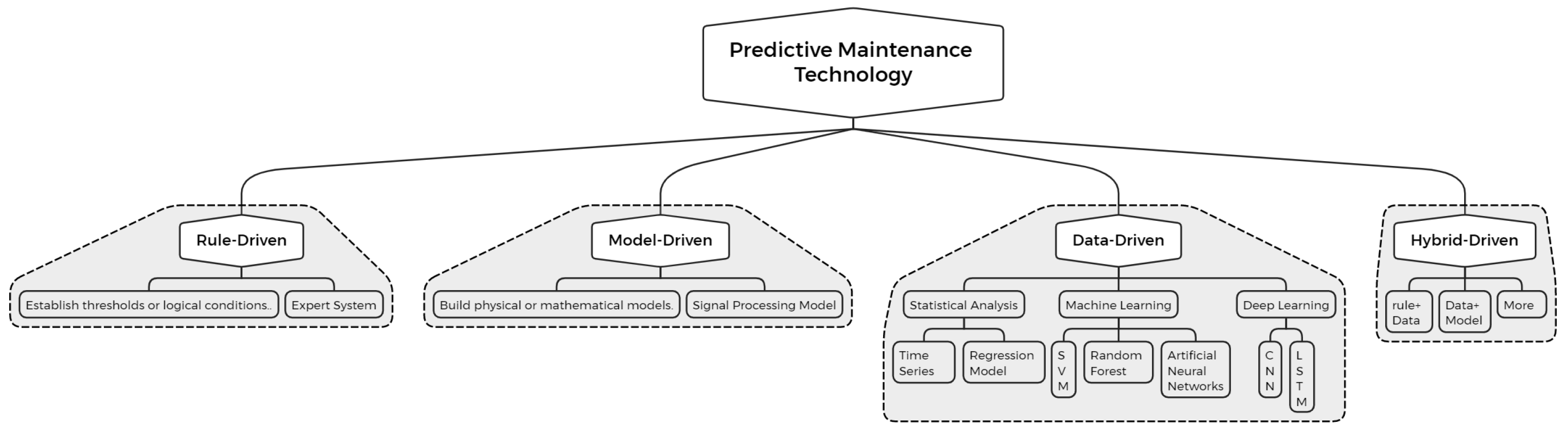
As illustrated in the figure, the proposed predictive maintenance method consists of three main components: data preprocessing, feature extraction, and fault classification. The data source includes sensor monitoring data from a specific iron-core current transformer located within a designated substation.
3.1. Data Preprocessing
In the predictive maintenance application discussed in this paper, the majority of the data sourced consists of time-series data from sensors. Therefore, it is crucial to conduct data preprocessing to effectively extract relevant features and eliminate noise and redundancy during the construction of the data analysis model.
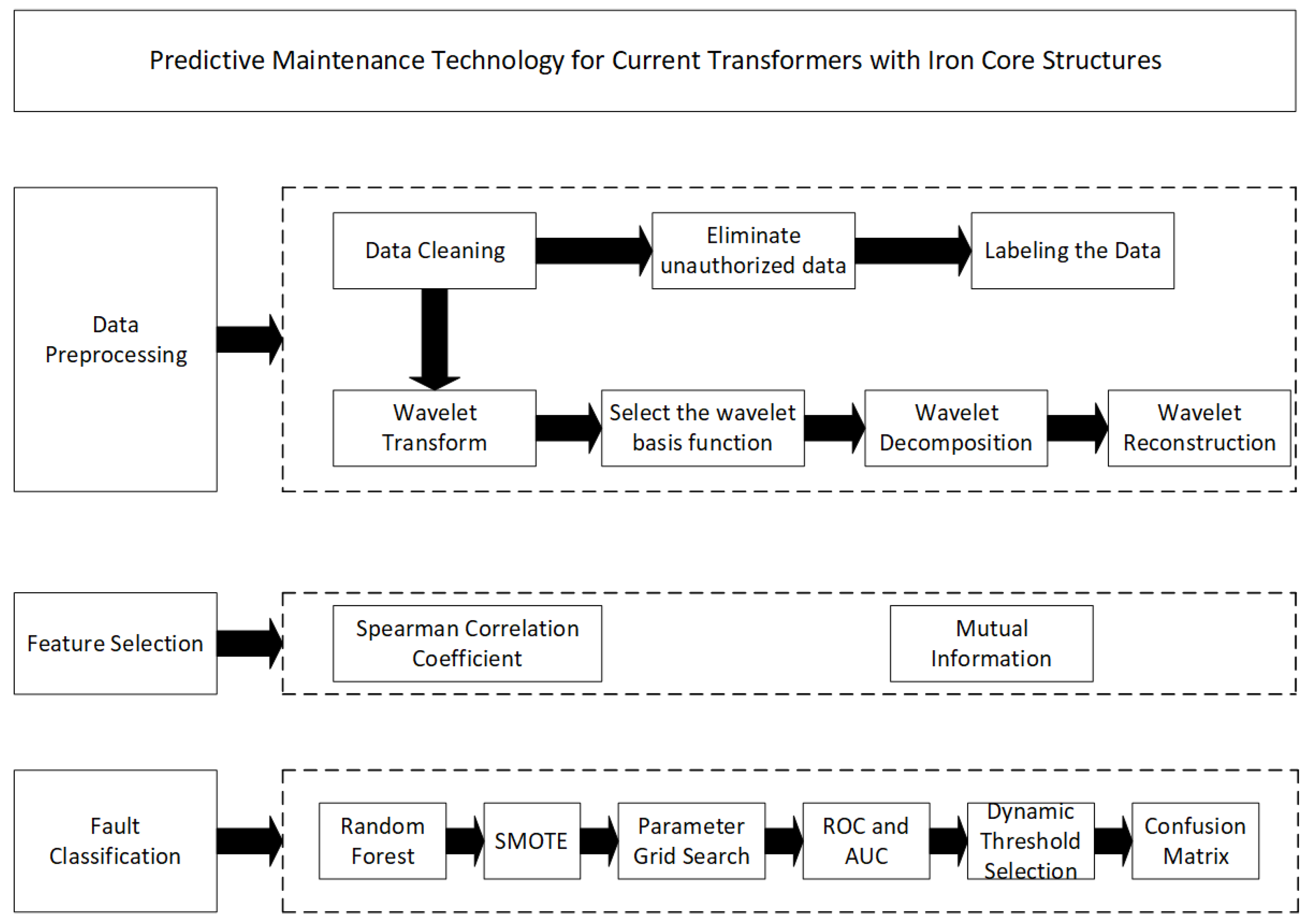
Regarding the data preprocessing phase, data cleaning is initially conducted to eliminate anomalous values and invalid data. Since the collected raw sensor data cannot be directly utilized for subsequent processing, data labeling is necessary to convert fault and healthy states into numerical forms that can be processed by machine learning models. In this context, we convert the labels “HLTY” (healthy state), “1HCF” (single-phase short-circuit fault state), and “2HCF” (double-phase short-circuit fault state) into numerical labels 0, 1, and 2, respectively. Furthermore, to process current transformer signals with complex frequency components and transient characteristics, this paper employs wavelet transform (WT) technology, which has demonstrated remarkable effectiveness in analyzing time-varying features or non-stationary signals [
22]. Prior to performing the wavelet transform, this study also processed the collected raw data. To extract statistical features, this research utilized a rolling window with a fixed size of 10 to capture overall trends and fluctuations in current, voltage, power factor, and other parameters. The reasoning behind the window selection was as follows:
- (1)
When extracting statistical features, choosing a sliding window with a fixed size of 10 shows relatively good performance in the experimental results, while the calculation time and memory consumption are relatively moderate.
- (2)
If a sliding window that is too large is used, some short-term changing features are likely to be smoothed out, which can negatively impact the detection capability of short-term faults and result in high computational time and memory consumption. Conversely, a sliding window that is too small may not adequately capture the changing features of the entire signal.
- (3)
We established the parameters based on the sampling frequency and detection window length of the power equipment in the substation. A window length of 10 is adequate to encompass a complete cycle of current fluctuation, thereby effectively extracting statistical features.
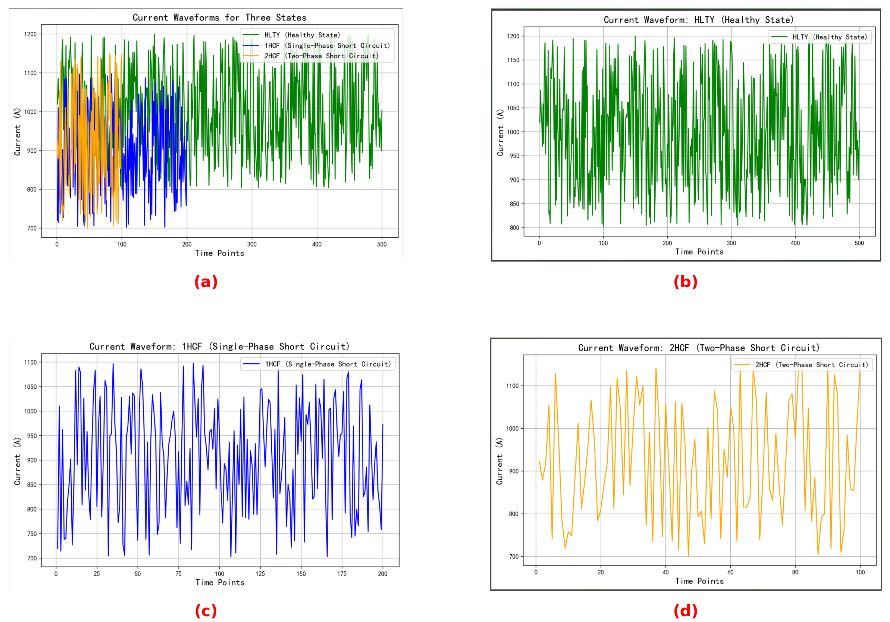
Figure 3 illustrates the current waveform diagram in its current state, as well as the current waveform diagrams for the three individual states.
The waveform diagrams above illustrate the variation of current values over time across three states. It is evident from the figure that the current waveform in the HLTY state is relatively stable, exhibiting a small amplitude range, with fluctuations approximately between 800 A and 1200 A. In contrast, the current waveform in the 1HCF state is more irregular, with fluctuations ranging from approximately 700 A to 1100 A. This irregularity may be attributed to current leakage resulting from a short circuit. The current waveform in the 2HCF state fluctuates between approximately 700 A and 1150 A, which is similar to the amplitude range of the 1HCF state; however, the fluctuation amplitude is greater than that of the 1HCF state, and the local peaks and valleys are more pronounced.
The wavelet transform in this research primarily consists of three key steps:
Step one involves selecting an appropriate wavelet basis function, denoted as . In this paper, we have chosen the Daubechies wavelet, which is widely utilized for signal decomposition and reconstruction as a filtering tool. This family of compactly supported wavelets is well-suited for the local analysis of signals and is capable of effectively capturing short-term variations in current transformer signals.
Step two involves wavelet decomposition. This study employs the Discrete Wavelet Transform (DWT), which decomposes current signals using a selected wavelet basis function into multiple levels of varying frequency components. This process allows for the extraction of signal features from different frequency bands. The signal can be represented as:
where
j represents the scaling parameter, indicating the various decomposition levels of the wavelet;
k is the translation parameter, denoting the translation position of the wavelet function in time or space;
is the wavelet coefficient, reflecting the outcome of the transformation at scale
j and position
k; and
is the wavelet basis function, adjusted by translation and scaling. Additionally,
J indicates the number of decomposition levels, and
is defined as follows:
Taking the collected current signal data from the current transformer as an example, we utilized wavelet decomposition to separate the current signal into low-frequency and high-frequency components, which represent the steady-state and instantaneous variation components of the signal, respectively. The low-frequency components, particularly those containing fundamental waves, are essential for detecting load changes and ensuring normal operations. The energy in the low-frequency portion typically correlates with the power system’s fundamental wave and load magnitude, while its mean and variance can reflect the average load level and fluctuations in load fluctuation conditions.
For larger j values, specifically the high-frequency components, the energy can indicate equipment failures or reveal the presence of high-frequency noise and transient signals. For example, during short-circuit faults, the current waveform may exhibit significant pulses and variations. These sudden changes in high-frequency components are captured, with statistical features such as peak values and spectral distribution reflecting these variations. Consequently, at each time point, wavelet decomposition is performed on the current data as well as the data from the previous nine time points. This process involves calculating the mean and standard deviation for low-frequency components, and skewness and kurtosis for high-frequency components. The features extracted after wavelet decomposition are retained for subsequent feature selection.
Step three involves wavelet reconstruction. This process is essential because, in classification prediction tasks, directly utilizing wavelet-decomposed current signals—decomposed into multiple layers with varying frequency components—can be overly complex and fragmented. Using all this frequency information directly as input for subsequent classification predictions is not appropriate. However, after reconstruction, the processed frequency domain information can be transformed back into signals that are suitable for further analysis, preserving the frequency information while enabling subsequent processing. We employ the Inverse Discrete Wavelet Transform (IDWT):
where
represents the wavelet coefficients obtained at the j-th level.
In this study, we selectively reconstructed the signal to retain only the low-frequency components, only the high-frequency components, and the fully reconstructed signal. This approach facilitates subsequent feature extraction and screening, followed by the selective input of the appropriate reconstructed signals into the classification training model.
The complete data preprocessing workflow is illustrated in
Figure 4.
The specifics of the operations are detailed in Algorithm 1.
| Algorithm 1 Data Preprocessing Algorithm |
- Require:
Raw dataset D, Wavelet type W - Ensure:
Processed dataset with numeric labels
- 1:
- 2:
for all do - 3:
if then - 4:
- 5:
end if - 6:
end for - 7:
- 8:
for all do - 9:
if is_healthy_data then - 10:
- 11:
else if is_single_phase_fault then - 12:
- 13:
else - 14:
- 15:
end if - 16:
- 17:
end for - 18:
- 19:
for all do - 20:
signal←extract_signal - 21:
- 22:
- 23:
- 24:
end for - 25:
return
|
3.2. Feature Selection
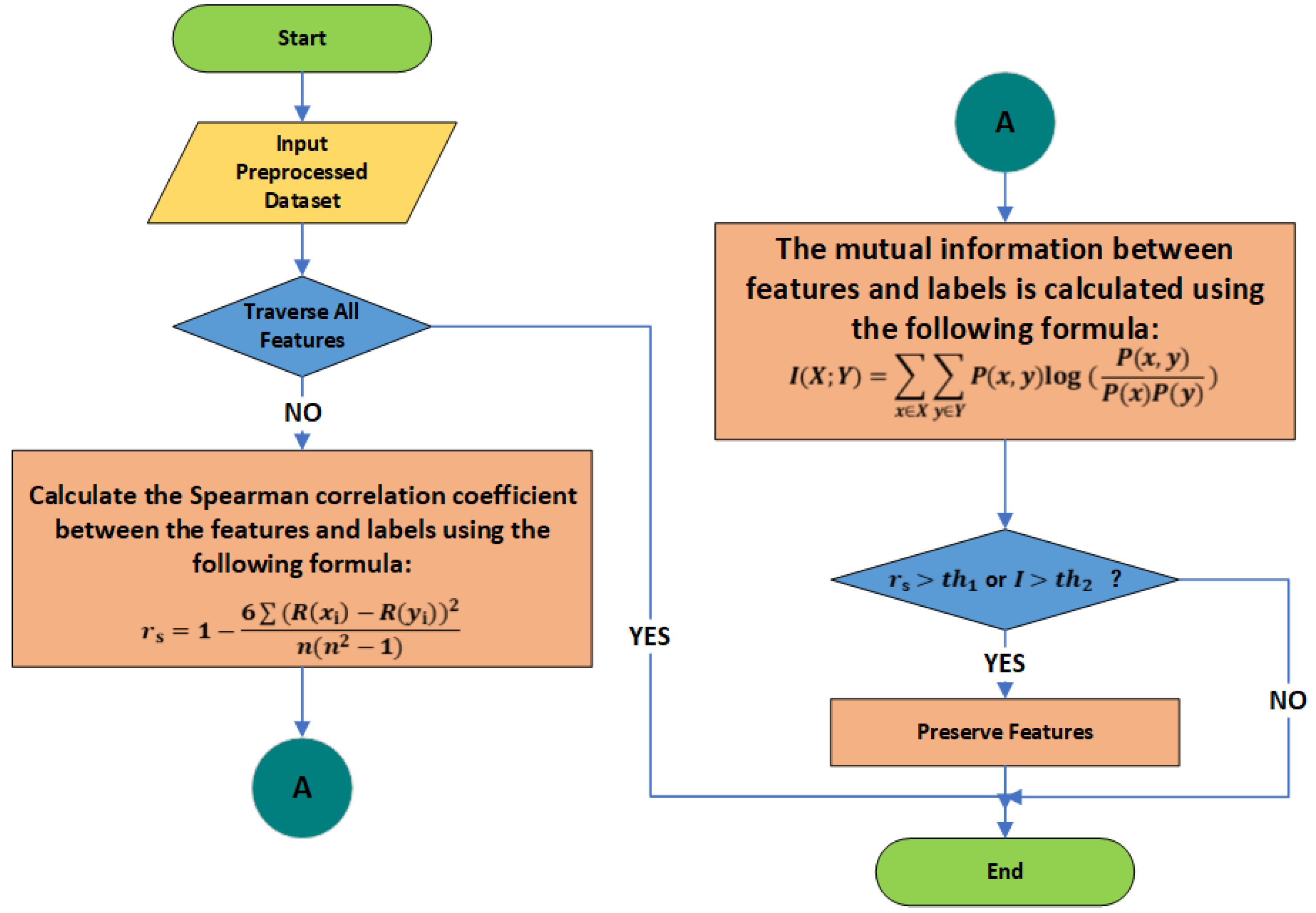
For feature extraction, this research employs a joint screening approach utilizing the Spearman coefficient (SC) and Mutual Information (MI). The Spearman coefficient is effective not only for linear relationships but also for monotonic non-linear relationships. In comparison to the Pearson correlation coefficient, it is less sensitive to outliers and can effectively reveal monotonicity between features and target variables. Meanwhile, Mutual Information measures the dependency between two random variables and captures more complex and potential non-linear associations. It is particularly adept at uncovering hidden relationships when the connections between features and target variables are intricate. By combining these two methods for screening, we can more comprehensively evaluate the correlation between features and target variables. This approach retains features that exhibit monotonic relationships with our state label classifications while also considering important non-linearly correlated features. Furthermore, when addressing complex data relationships, this joint approach helps mitigate certain biases in feature selection. The screening conducted from different dimensions using these two methods can enhance our model’s generalization capability, resulting in more accurate and stable training and prediction outcomes.
The specific methodology is illustrated in
Figure 5.
The definitions of R() and R() in the figure are as follows:
R() is a ranking value generated by sorting a single feature extracted from the historical monitoring data of the current transformer using wavelet transformation or statistical feature extraction. The monitoring data include current values, voltage values, power factors, temperature, humidity, harmonic content, and load status. The extracted statistical features encompass characteristic values such as the mean, standard deviation, kurtosis, and skewness. Here, represents all the extracted characteristic values. The advantage of the ranking value R() over the calculation of absolute values is that it can eliminate the influence of units from different physical variables.
R() represents the ranking value obtained by sorting the state samples of the current transformer. Here, denotes the target state label, which corresponds to the current transformer’s state. The possible state labels include healthy state (HLTY), single-phase short circuit fault (1HCF), and double-phase short circuit fault (2HCF). These states are converted and represented by digital labels: 2 for healthy state, 0 for single-phase short circuit fault, and 1 for double-phase short circuit fault.
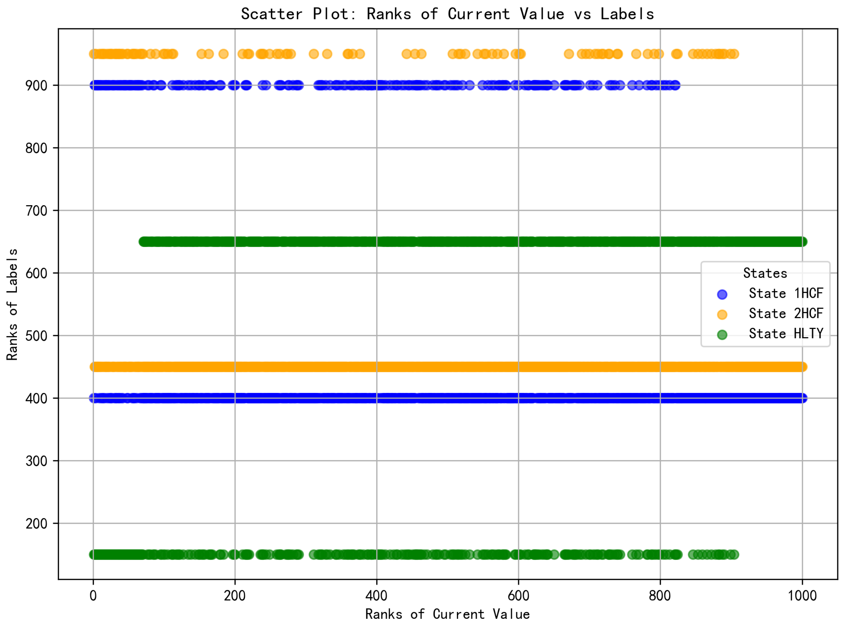
In order to more clearly illustrate the ranking distribution and correlation between R(
) and R(
), we use the characteristic of
, which represents the current value, as an example for demonstration and explanation in
Figure 6.
The scatter plot above illustrates the relationship between the ranking distribution of the current value feature and the state label rankings. The horizontal axis represents the feature ranking of the current value, where a higher ranking value indicates a greater current value of the sample. The vertical axis denotes the ranking of the state labels (HLTY, 1HCF, 2HCF). Each label is discretized and represented by a numerical value, with the ranking of each state calculated based on the binary (0,1) label of the corresponding sample. Specifically, if a sample belongs to a particular state label, its corresponding value is 1, resulting in a higher ranking value. Conversely, if the sample does not belong to that state label, the value is 0, leading to a lower ranking value.
The data points for different states in the figure are represented by distinct colors: blue indicates 1HCF, yellow signifies 2HCF, and green denotes HLTY. The distribution illustrated in the figure reveals a significant overlap between the blue and orange points in certain areas, suggesting that the 1HCF and 2HCF states share similarities in their current value distributions. This overlap may pose challenges for the classifier in differentiating between the two states, thereby impacting the model’s predictive performance. Consequently, this is one of the factors contributing to the low prediction accuracy of 2HCF.
The statistical features extracted after the wavelet transform, including the mean and standard deviation, along with reconstructed signals and other feature data, are incorporated into the target feature set (featureSet) for iteration. The process then iterates through the feature set (featureSet), calculating both the Spearman coefficient and the Mutual Information coefficient between each
and the target values (i.e., the digitized state labels) according to the corresponding mathematical formulas presented in
Figure 5.
Further screening is conducted using the Spearman coefficient to eliminate features that exhibit minimal monotonic relationships with the labels. For instance, during feature iteration, calculations indicated that the mean and variance of current values derived from low-frequency components extracted through wavelet transform demonstrated high Spearman coefficient values when assessed against state label values, highlighting clear distinctions between healthy and faulty states. Conversely, features such as harmonic content and power factor produced results close to zero, suggesting no significant monotonic relationship for state discrimination. This step preliminarily reduces data dimensionality while preserving features with strong monotonic relationships. However, in practical scenarios, variables often possess more complex relationships that cannot be adequately captured by monotonicity alone. Therefore, relying solely on the Spearman coefficient is insufficient; it is essential to incorporate Mutual Information to assess non-linear relationships, thereby preventing the exclusion of important features that could impact the training accuracy and reliability of subsequent fault classification models.
After preliminary screening, we utilize Mutual Information to assess whether the remaining features exhibit non-linear or more complex effects on the labels. If there is no information overlap between the currently examined feature and the state label values, the calculated value of the formula is 0. Conversely, if the features are completely correlated, the Mutual Information equals their entropy. Some features may not demonstrate significant performance in the Spearman coefficient during preliminary screening but may perform well in the Mutual Information assessment. Such features should not be overlooked, as they may possess important predictive capabilities.
In the feature selection process, setting appropriate thresholds is crucial for decision-making, as it directly influences the ability of selected features to effectively support model training and enhance prediction accuracy. Establishing suitable thresholds helps eliminate irrelevant or noisy features while retaining those that positively contribute to model performance. In this context, for the Spearman coefficient threshold (Threshold 1), we determined that an absolute value of the Spearman coefficient between 0.2 and 0.3 typically indicates a moderate monotonic relationship between features and labels. In contrast, values ranging from 0.5 to 0.7 demonstrate a very strong monotonic relationship. To eliminate features with extremely weak relationships to state label values while avoiding the exclusion of effective features due to excessively high threshold settings, we established the final Threshold 1 at 0.3. For Mutual Information (Threshold 2), we noted that, in most cases, features with lower Mutual Information values exert a weaker influence on target labels, whereas features with higher Mutual Information values generally possess greater predictive capability for those labels. To prevent overlooking non-linear relationships while filtering out features with evidently weak non-linear relationships, we set Threshold 2 at 0.1.
Finally, during the screening process, we selected features that met either the specified Threshold 1 for the Spearman coefficient or Threshold 2 for Mutual Information.
3.3. Classification Prediction
For the classification prediction component, we utilize a Random Forest model. This model exhibits the characteristics of ensemble learning, providing high accuracy and robustness while effectively managing high-dimensional data and noise. It also offers excellent parallelization capabilities and can assess feature importance, showcasing its strong problem-solving abilities for complex, non-linear state data of current transformers.
The specific steps are outlined as follows:
After completing preprocessing and feature selection, we divide the data into training and test sets. First, we create a model using a pipeline that incorporates SMOTE (Synthetic Minority Over-sampling Technique) and a Random Forest classifier. Since the substation discussed in this paper operates without equipment failures most of the time, the fault data in the collected current transformer data represent a small minority. This situation can hinder the model’s ability to effectively learn the characteristics of fault data during training, leading to a class imbalance problem. Therefore, SMOTE is employed to generate additional samples of the minority class, thereby achieving a more balanced training dataset.
The next step involves hyperparameter optimization. We utilize grid search in conjunction with cross-validation to identify the optimal combination of hyperparameters for the model. Subsequently, we apply this optimal combination to make predictions on the test set.
After identifying the optimal parameter combination through grid search, we train the optimized pipeline using the training set. Upon completion of the training process, we utilize the method to calculate the probability of each sample belonging to each class. These probability data serve as the foundation for subsequent evaluations of model performance.
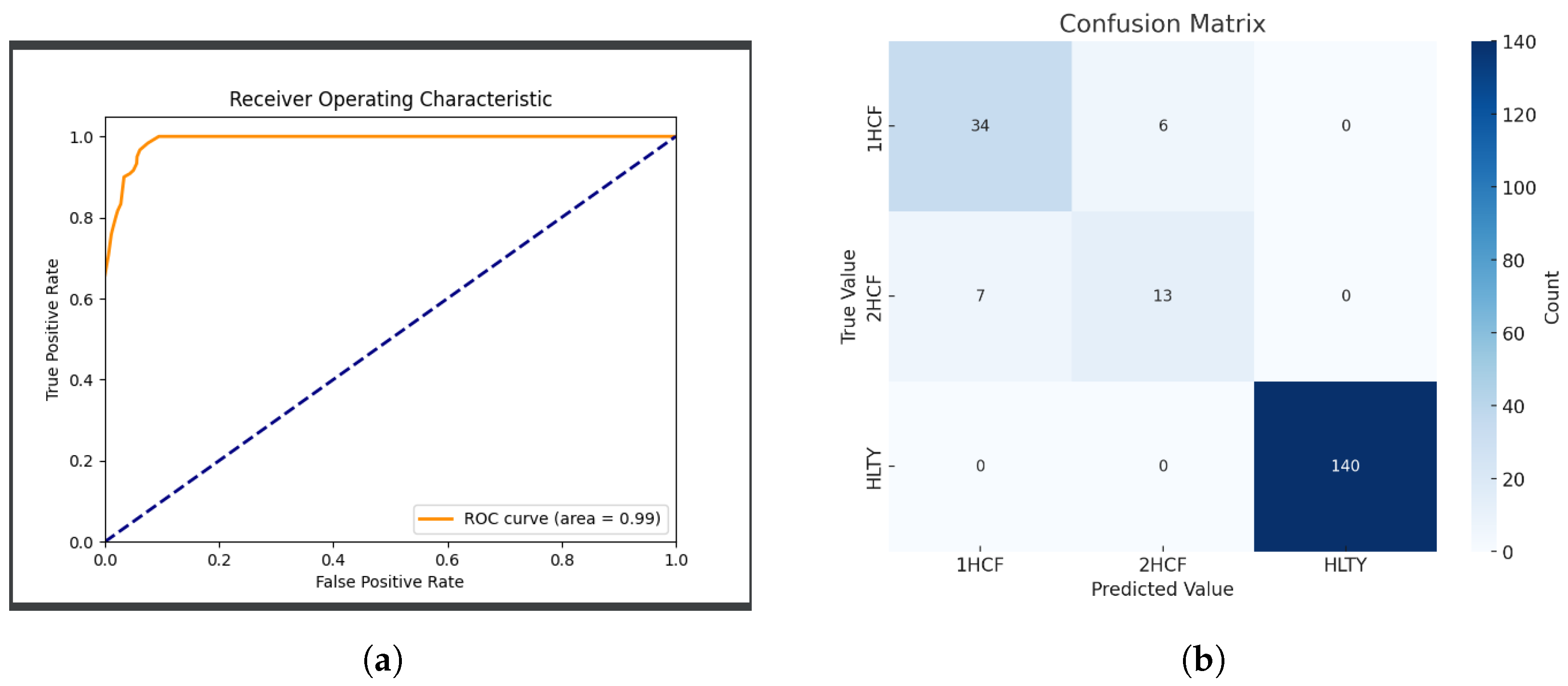
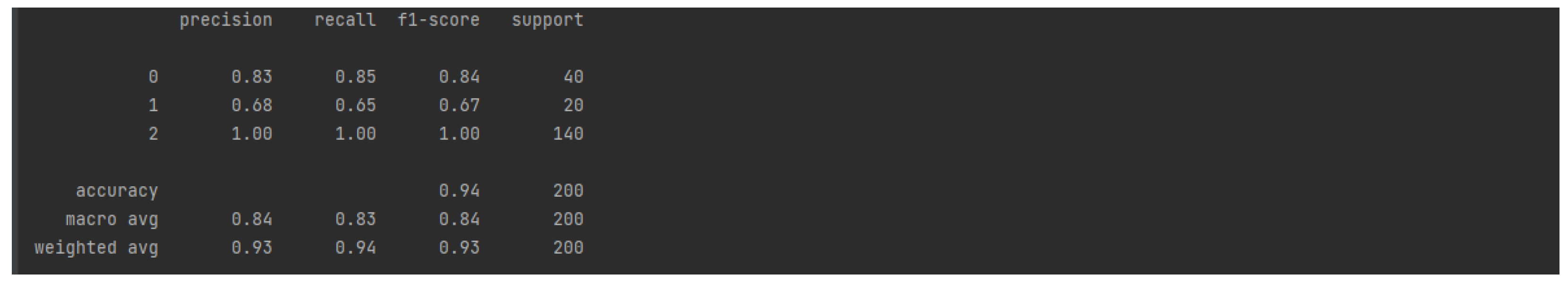
Finally, we conduct a comprehensive evaluation of model performance. This paper calculates the Receiver Operating Characteristic (ROC) curve for each class and computes the macro-average ROC Area Under the Curve (AUC) metric, generating corresponding ROC curve plots. By plotting the relationship between the True Positive Rate (TPR) and the False Positive Rate (FPR), we illustrate the classifier’s ability to differentiate between positive and negative samples.
Based on the Receiver Operating Characteristic (ROC) curve, we dynamically select the optimal threshold to enhance the model’s predictive performance. Subsequently, we generate a confusion matrix to illustrate the comparison between predicted and actual results for each class, thereby revealing the accuracy and reliability of the pre-trained model in predicting real samples.
The specifics of the feature selection and classification prediction training operations are outlined in Algorithm 2.
| Algorithm 2 Feature Selection and Model Training for Fault Diagnosis |
- Require:
Processed dataset , MIC threshold , Model type M - Ensure:
Trained model
- 1:
- 2:
Step 1: Feature Selection - 3:
for all do - 4:
- 5:
for all do - 6:
- 7:
if then - 8:
- 9:
end if - 10:
end for - 11:
end for - 12:
Step 2: Train-Test Split - 13:
- 14:
Step 3: Model Training - 15:
- 16:
- 17:
Step 4: Model Evaluation - 18:
- 19:
- 20:
- 21:
- 22:
return
|


