PDNet by Partial Deep Convolution: A Better Lightweight Detector

Abstract

Model lightweighting is significant in edge computing and mobile devices. Current studies on fast network design mainly focuses on model computation compression and speedup. Many models aim to compress models by dealing with redundant feature maps. However, most of these methods choose to preserve the feature maps with simple manipulations and do not effectively reduce redundant feature maps. This paper proposes a new convolution module, PDConv, which compresses redundant feature maps to reduce network complexity and increase network width to maintain accuracy. PDConv (Partial Deep Convolution) outperforms traditional methods in handling redundant feature maps, particularly in deep networks. Its FLOPs are comparable to deep separable convolution but with higher accuracy. This paper proposes PDBottleNeck and PDC2f (Partial Deep CSPDarknet53 to 2-Stage FPN) and build the lightweight network PDNet for experimental validation using the PASCAL VOC dataset. Compared to the popular HorNet, our method achieves an improvement of more than 25% in FLOPs and 1.8% in mAP50:95 accuracy. On the CoCo2017 dataset, our large PDNet achieves a 0.5% improvement in mAP75 and lower FLOPs than the latest RepVit.

1. Introduction

Lightweight object detection models have become a highly anticipated trend in computer vision in recent years. They significantly reduce computational complexity and resource consumption while maintaining high accuracy. These advantages bring multiple benefits, including real-time performance, broad applicability, cost and energy savings, and enhanced user experience. As a result, lightweight models have become one of the most prominent cutting-edge technologies in computer vision, receiving widespread attention and applications.

However, achieving both high accuracy and efficiency remains a critical challenge. Many lightweight models adopt depthwise convolution (DW) to improve speed, but relying solely on DW sacrifices accuracy due to its inability to effectively fuse inter-channel information or fully utilize spatial features. MobileNets [1,2,3] introduces Pointwise Convolution (PW) to fuse inter-channel features, while ShuffleNets [4,5] enhances performance through channel reorganization. However, these approaches have limitations, such as additional computational overhead from PW or instability in practical channel reorganization.

In addition, the redundancy of feature maps is a critical issue that is often overlooked in lightweight model research. By observing feature maps, this paper found that some exhibit a high degree of similarity, and simply retaining these features using low-cost operations does not resolve the problem but rather leads to redundant information. While existing methods have made progress in reducing computational complexity, they often fall short in effectively leveraging feature representation. For instance, GhostNet [6] reduces model complexity by generating cheap feature maps but fails to fully eliminate redundant features. Additionally, many approaches attempt to compensate for accuracy loss by increasing network width, which typically incurs higher memory access overhead, making them less practical for low-power devices.

To address these challenges, this paper proposed a novel strategy based on compressing redundant feature maps, complemented by network width enhancement to optimize feature representation and achieve a balance between accuracy and efficiency. Building on this strategy, this paper designed a new convolution method, PDConv, which significantly reduces network complexity by retaining only a portion of the redundant feature maps. Leveraging this method, this paper constructed an efficient neural network, PDNet (Figure 1). Experimental results demonstrate that PDNet achieves notable accuracy improvements while maintaining high efficiency, highlighting the effectiveness of the proposed approach. Our contributions are as follows:

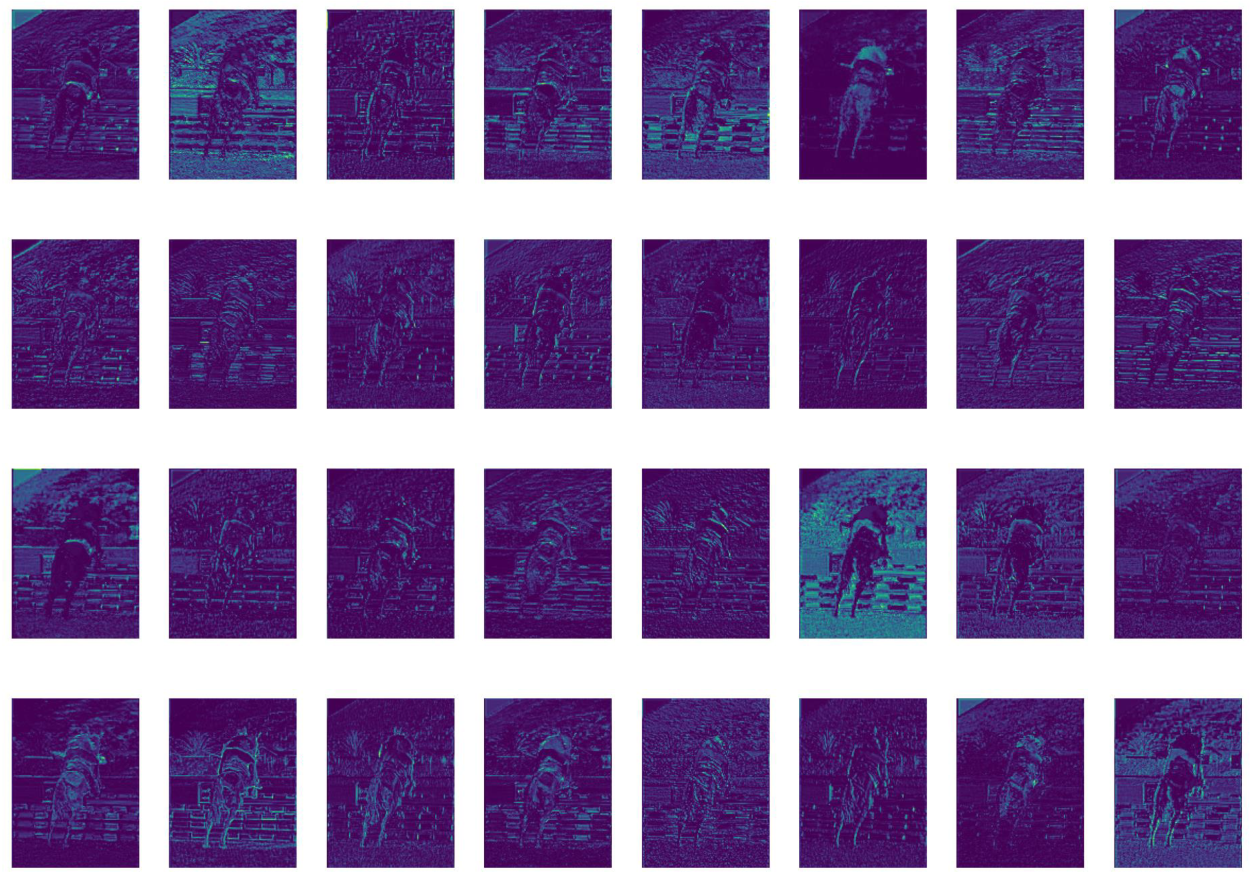
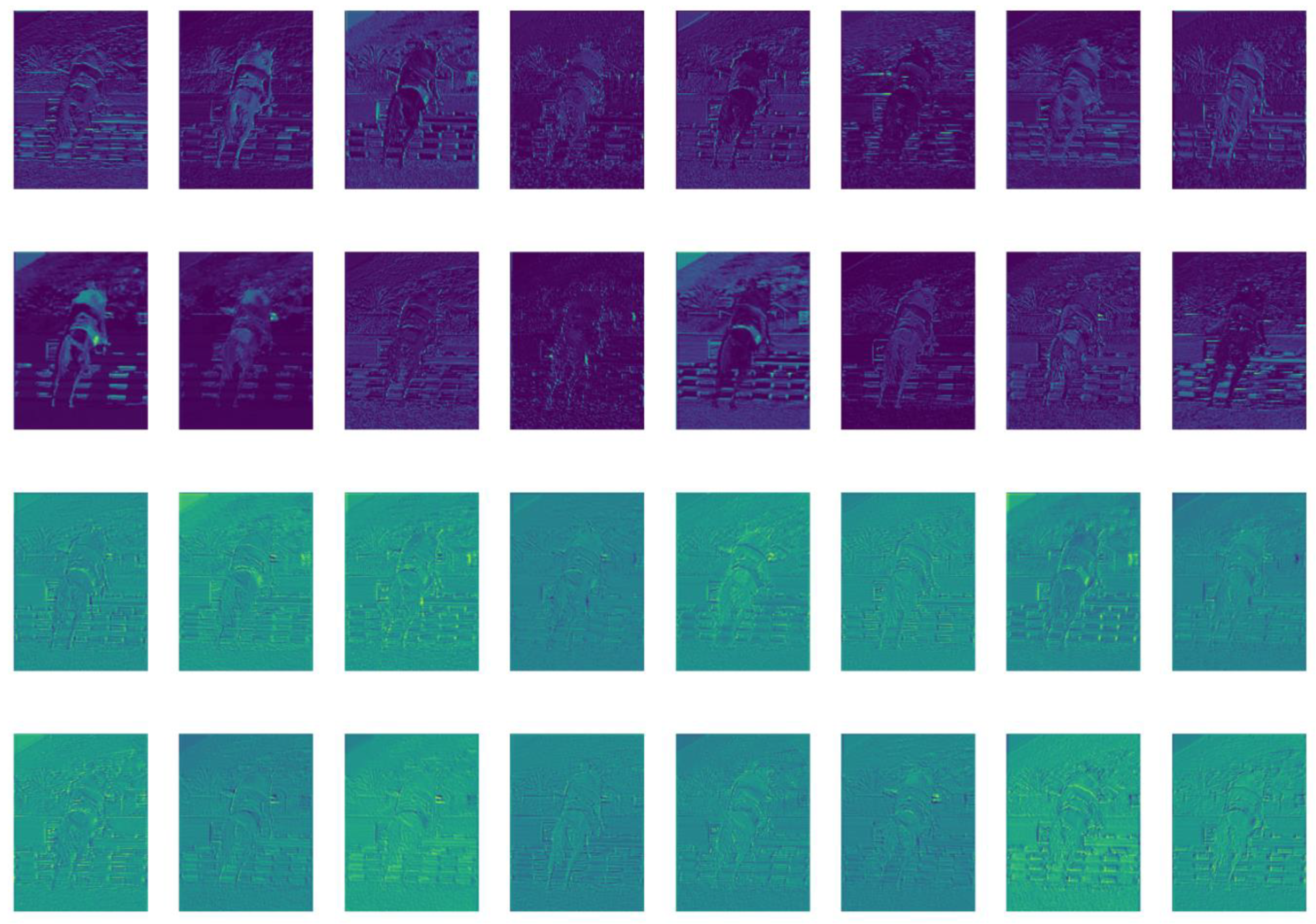
• In the process of feature map generation, this paper introduced a new idea: retaining only part of the redundant feature maps can achieve similar results as retaining all the redundant feature maps completely. This idea explores a new way of dealing with feature map redundancy, aiming to improve the efficiency of the model while maximising the retention of key information.
• This paper proposed a lightweight convolutional module, PDConv, which is designed to reduce the complexity of the model. PDConv is capable of removing part of the redundant feature maps, thus reducing the number of parameters and computational burden of the network while maintaining the model performance.
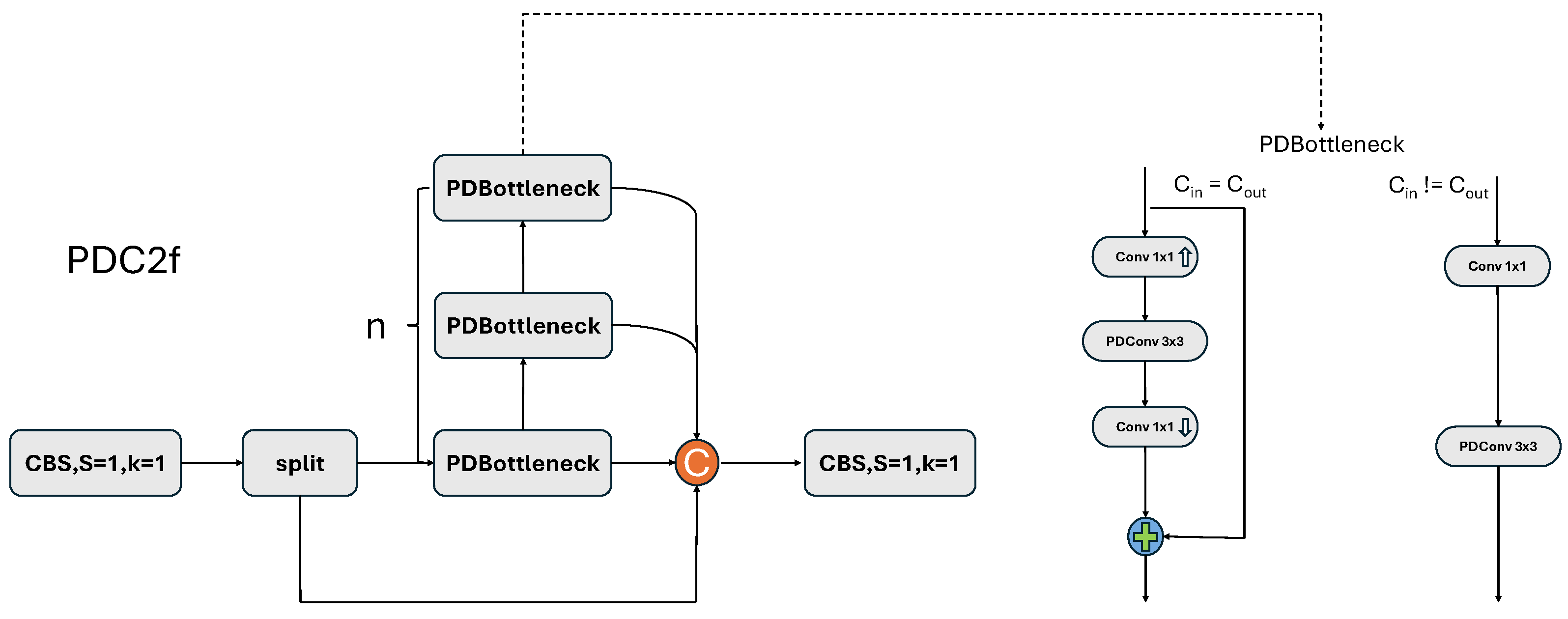
• Based on PDConv, this paper has designed a more suitable PDBottleneck and PDC2f structure to better exploit the characteristics of PDConv.
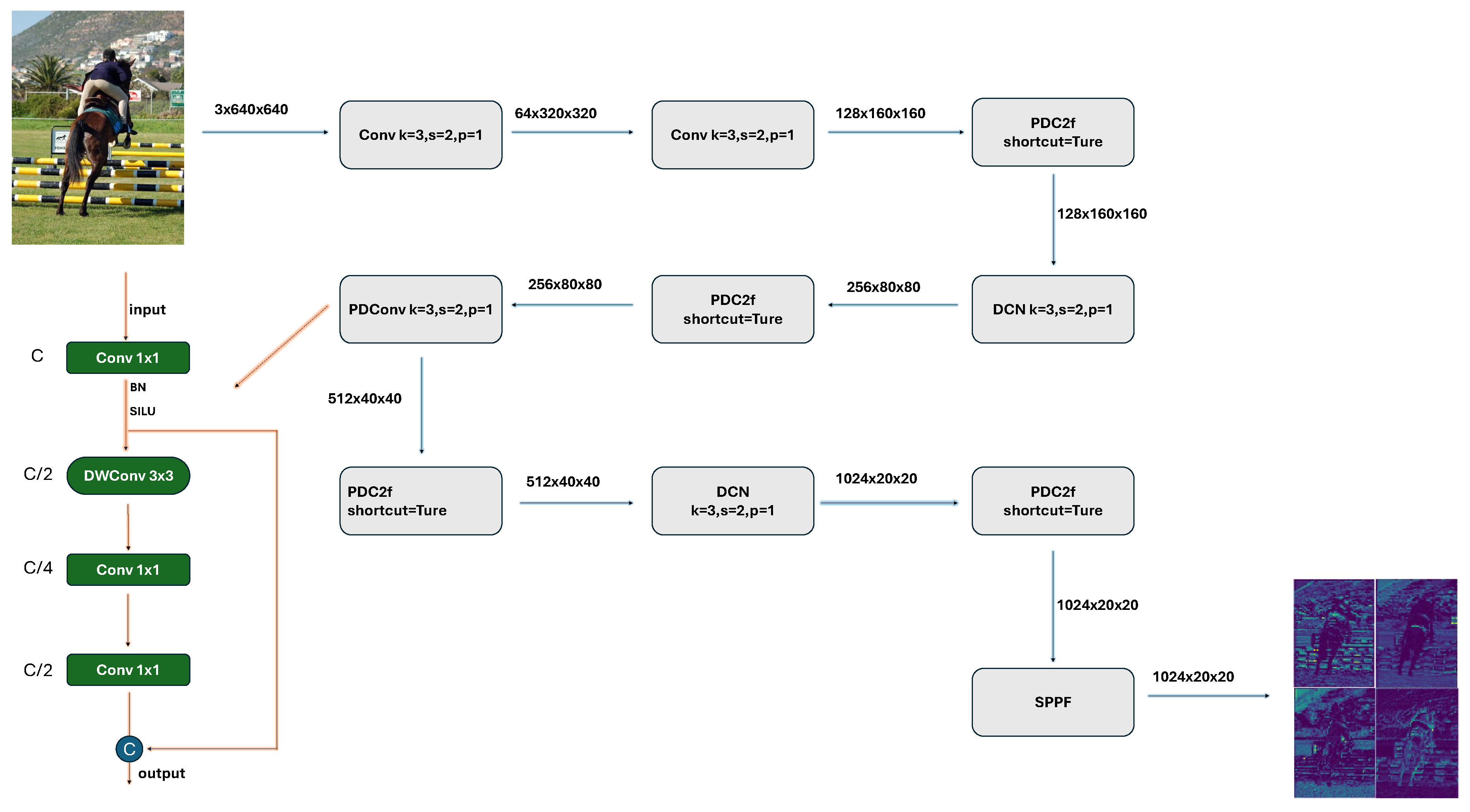
• This paper constructed a lightweight network structure, PDNet, which integrates PDConv, PDBottleneck, and PDC2f modules and achieves the goal of reducing model complexity while maintaining accuracy in feature extraction through well-designed connections and parameter settings.

The rest of the paper is organised as follows: Section 2 briefly describes the work related to the lightweight design of the detector, Section 3 details our proposed PDConv as well as the PDNet, Section 4 presents the results of our experiments, Section 5 summarizes the limitations of our proposed PDConv and future work, and a final conclusion is given in Section 6.

2. Related Work

With the widespread application of deep learning models in computer vision and other tasks, reducing the model’s computational load and storage requirements without significantly sacrificing performance has become a research hotspot. Lightweight network architecture design is an important approach to addressing this challenge. Unlike traditional model compression methods (such as pruning and quantization), lightweight architecture design optimizes the model’s computational and storage efficiency by modifying the network structure itself.

To explore faster networks, the discussion begins with the CNN architecture. Refs. [7,8,9,10,11,12,13] worked by using deep convolution or improved deep convolution, which is probably the most popular method at the moment, but, as mentioned above, there can be a problem in not being able to fuse the information between channels; therefore, MobileNets [1,2,3] introduces Pointwise Convolution (PW), which uses a 1 × 1 convolution to fuse the feature maps between channels. ShuffleNets [4,5] enhances the effect by disrupting the channel reorganisation approach to promote better information exchanges between channels. These strategies proved effective. Ghost [6], on the other hand, generates cheap feature maps by halving the SC, but this introduces an additional 1 × 1 convolution, resulting in no significant improvement in inference speed despite the reduction in model complexity.

In addition, PConv uses the application of Conv on only a portion of the channels without affecting the other channels through partial SC operation. There are also many lightweight models, such as EfficientNets [14,15], TinyNet [16], CondenseNets [17,18], TVConv [19], MnasNet [20], and FBNets [21,22,23,24]. All these nets have one thing in common, i.e., they use different methods to minimise the resources consumed for feature extraction in order to achieve the lightweight model. However, they tend to increase the width of the network to compensate for the accuracy, which is affected by the increased memory access in some limited devices. Instead, this paper proposed to reduce the network complexity by compressing some of the redundant features and then improve the feature representation by increasing the network width, which compensates for the increase in memory access and feature specificity caused by simply increasing the network width.

Since the application of Vision Transformer (VIT) to the field of computer vision, many subsequent works have attempted to provide a better understanding of VIT in training settings [25,26] and model design [27,28,29] in order to improve VIT. Refs. [30,31,32] reduces the burden on the network by reducing the attention operator, while [33,34,35] suggests replacing attention with simple MLP-based operators instead of attention, but this often evolves into CNN-like architectures.

In this paper, VIT is not our focus of research; this is because convolutions based on the attention mechanism tend to result in slower operation, and, in autonomous driving and edge devices, the deep convolution-based lightweight model is still the mainstream choice.

3. Principles and Methods

3.1. HOW PDConv

Before delving into the proposed research, it is essential to examine the image in Figure 2, which illustrates the feature maps obtained through two-layer SC extraction. The image highlights the presence of similar or even identical patterns among multiple feature maps, a phenomenon referred to as feature redundancy. Addressing this redundancy without compromising the network’s performance has been a critical challenge. A review of existing lightweight convolution methods has revealed that halved SC is a promising approach, where half of the channels remain unprocessed and the other half undergo lightweight operations. For instance, Ghost Conv utilizes inexpensive operations, GSConv [36] incorporates depthwise convolution and channel shuffling, and PConv selectively convolves only a portion of the channels, leaving others unchanged. Drawing inspiration from these methods, PDConv is proposed as a novel approach to efficiently mitigate feature redundancy.

For the input feature map, the number of channels is first halved using a 1 × 1 convolution, i.e., a convolution kernel where half the number of channels is set. The dimension of the input tensor X is [H, W, 2C], where H denotes the height, W the width, and 2C the number of input channels. We assume that there exists a 1 × 1 convolution kernel K with dimensions [1, 1, C]. The output Y1 of the 1 × 1 convolution can be expressed as follows:

$$Y_1=\sum _{i=0}^{C-1}X·K[1,1,i]$$

(1)

In the above expression, $Y_1$ represents the output of the 1 × 1 convolution, i represents the index of the input channel, and $K[1,1,i]$ represents the weights of the 1 × 1 convolution kernel. The 1 × 1 convolution performs a weighted combination of the input channel’s features at each position and then generates the output channel’s features. This operation results in a generated feature map with half the number of channels, i.e., C. Then, a DW convolution is performed on half of the number of channels using a convolution kernel of size k × k, typically 3 × 3. The output tensor of this operation has dimensions [H, W, C] and can be denoted as:

$$Y_2=\sum _{i=0}^{C-1}{Y}_1^{\left(i\right)}·K[k,k,i]$$

(2)

$Y_1^{\left(i\right)}$ represents the cth group into which the output of Equation (1) is divided. When performing a 1 × 1 convolution operation on the feature map after DW convolution, this paper aims to make full use of the spatial information at different locations. The number of convolution kernels for this convolution operation is set to one-half of the number of input channels, i.e., C/2. Therefore, the final number of channels of the feature map is only one-fourth of the initial number of input channels after the weighted combination, similar to downsampling. One might be concerned about whether the reduced number of channels would lead to a loss of information. However, when this paper examines the actual situation more closely, it will be clearly found that, although this paper has downsampled the number of channels, this specific operation is carried out after the depthwise separable convolution (DW convolution). The main purpose of the DW convolution is to comprehensively integrate the information dispersed among different channels, eliminate redundancies, and extract the most valuable data. Therefore, by the time the downsampling step is performed, the feature map has already been refined to a certain extent, so the impact of downsampling on it is much smaller than what people initially assumed.

In the final stage, the last generated feature map is uplifted and spliced with the feature map $Y_1$ produced by Equation (1) to form a complete feature map. A potential question is why $Y_1$ was not removed and was, instead, spliced. The rationale behind this choice is that removing $Y_1$ would reduce the convolution to a depthwise separable convolution with a limited number of channels, leading to a loss of accuracy. Such a reduction would contradict the design philosophy, which aims to minimize feature map redundancy without compromising the model’s feature generation capacity. The objective is to retain the richness of the overall feature map, ensuring that sufficient feature information remains rather than processing only part of the feature map. By retaining and splicing $Y_1$, the information richness of the network is preserved, which contributes to maintaining the model integrity. This approach ensures that feature extraction and information representation remain comprehensive, thus upholding the performance of the model.

The feature maps generated after two PDConv processes exhibit significantly fewer redundant features, (see Figure 3). This change is evident. It is worth noting that, during feature extraction, these feature maps are less sensitive to aspects such as colour background and more sensitive to features such as target contours. In fact, this type of feature extraction is closer to biology and is similar to the way the animal visual system works.

3.2. Computational Complexity

In the last section, this paper introduced PDConv as a lightweight convolution designed to reduce feature redundancy while maintaining network performance. To evaluate the effectiveness of this design, it is crucial to analyze its computational complexity. The computational cost of a convolution operation is typically measured using floating point operations (FLOPs), and the amount of computation depends on the size of the input feature map, the size of the convolution kernel, and the size of the output feature map. Therefore, understanding the computational cost of PDConv is essential for verifying its ability to reduce computational resources while maintaining efficiency. For regular 2D convolution, the general formula for calculating FLOPs is as follows: when the number of input channels is $C_{in}$, the size of the convolution kernel is K, the number of output channels is $C_{out}$, and the size of the output feature map is H × W, then the formula without considering the bias can be obtained as

$$\mathrm{FLOPs}\text{\_}\mathrm{SC}=2·C_{\mathrm{in}}·C_{\mathrm{out}}·K·K·H·W$$

(3)

This gives us the formula for FLOPs, which is split into 4 parts due to its complexity. The first step is the first dimensionality reduction, where the convolution used is 1 × 1, so K = 1, and the output channel is 1/2 of the input channel, i.e., $C_{in}$ = 2$C_{out}$.

$${\mathrm{FLOPs}}_1=C_{\mathrm{in}}·C_{\mathrm{out}}·H·W$$

(4)

The second step performs one DW convolution of the reduced feature map with the convolution kernel size K (usually 3), and the computational cost of this part can be expressed as

$${\mathrm{FLOPs}}_2=C_{\mathrm{in}}·K·K·H·W$$

(5)

The third step accumulates the same position information from different spaces, and the output channel, which is 1/2 of the input channel, here $C_{out}$/2, is used to denote the output channel, while the convolution kernel is 1 × 1; therefore, it is expressed as

$${\mathrm{FLOPs}}_3={\displaystyle \frac{C_{\mathrm{in}}·C_{\mathrm{out}}}{2}}·H·W$$

(6)

The fourth step performs the upscaling; the convolution kernel used is 1 × 1, the input channel is $C_{in}/2$, and the output channel is $C_{out}$, and so the expression is

$${\mathrm{FLOPs}}_4={\displaystyle \frac{C_{\mathrm{in}}·C_{\mathrm{out}}}{2}}·H·W$$

(7)

Note that this paper uses the same padding strategy in each convolution process so that the image size maintains H * W constant. Then, the computational complexity ratio of PDConv to SC is

$$r={\displaystyle \frac{1}{K^2}}+{\displaystyle \frac{1}{2C_{\mathrm{out}}}}\approx {\displaystyle \frac{1}{K^2}}$$

(8)

This value is approximately equal to the depth of separable convolution.

3.3. Building PDC2f

In Convolutional Neural Networks (CNNs), the number of channels in the feature map of the backbone network gradually increases as the depth of the network increases and the spatial resolution gradually decreases. In this process, when using PDConv to process the feature maps, the complete extraction of information may be adversely affected due to the decrease in the number of channels. In order to solve this problem while taking into account the lightweight design of the network, this paper proposes the PDC2f module (shown in Figure 4) for further optimising the feature processing capability after PDConv. The core component of PDC2f is the PDBottleNeck, which enhances the feature expression capability through multi-level feature manipulation.

Specifically, in the backbone network, PDBottleNeck increases the number of channels of the feature map by channel expansion when the number of input channels and the number of output channels are the same. This design allows the network to extract richer abstract features. Each channel can be considered as a unique feature representation of the input data, and an increase in the number of channels equates to the network being able to capture a more diverse pattern of features. This is important for the improvement of feature extraction and representation in the backbone network, as well as in regard to providing more comprehensive feature support for subsequent network layers.

In addition, PDConv selectively focuses on key regions through its dynamic sampling mechanism, thus effectively improving the flexibility of feature extraction. However, relying only on PDConv may result in missing some of the fine-grained information on the high-resolution feature maps. Therefore, the combination of PDC2f and PDConv can compensate the information loss while lightweighting and provide stronger feature expression.PDBottleNeck plays a bridging role, enriching the feature expression through channel expansion on one hand and reducing the risk of gradient disappearance by using residual connectivity on the other hand to maintain the coherence of the information flow.

However, at the neck layer of the network, the marginal gain of channel expansion is smaller due to the already high channel dimension of the feature graph. This is because the feature graph has already formed a relatively high dimensional representation at this stage and further increasing the number of channels may lead to additional computational complexity without significantly improving the representation capability. Meanwhile, the shape of the feature maps in the neck layer tends to be more elongated (similar to a rope-like structure), in which case the usefulness of channel expansion is limited. Therefore, in this paper, we choose not to perform channel expansion in the neck layer in order to avoid unnecessary computational overheads, thus striking a balance between performance and efficiency.

3.4. Building Efficient Net

In order to optimise the computational speed in Convolutional Neural Networks (CNNs), it is often necessary to perform a series of transformation processes on the input image in the backbone part of the network. The goal of these transformation processes is to gradually transform spatial information into channel information. However, each compression of the spatial dimensions (width and height) and expansion of the channels on the feature map may result in partial loss of semantic information. The use of DSC may lead to excessive loss of semantic information and thus lead to a significant decrease in the accuracy; therefore, in this paper, this article designed a backbone based on PDConv. Its structure is shown in Figure 1. This article borrows CSPDarkNet [37] and equips it with an advanced detection head of YOLOv8, based on which it constructs a more efficient PDNet.

In order to highlight the extent to which the neural network contributes to different regions of the image, as well as to highlight the relative importance and activity of these regions, this article selected two images from the PASCAL VOC dataset and generated heat maps (similar to the attention mechanism) (Figure 5). These heat maps clearly show the regions where the network contributes more to the prediction results and enable an intuitive understanding of the key regions on which the model bases its decision-making. This article makes the detection results clearer by merging the results of object detection and the heat maps.

4. Experiments

In this section, this article describes in detail the dataset used for our experiments and the configuration of the experimental environment. Additionally, we show the results of the experiments that were carried out.

4.1. Experiment on PASCAL VOC

This article chose the PASCAL VOC2007+2012 [38] dataset, one of the most widely used datasets for object detection, which includes four major classes (vehicle, household, animal, and person) as well as 20 subclasses (plus one for background). The combined VOC2007 and VOC2012 datasets provide a large number of labeled images. For training and validation, this article used the VOC2007 and VOC2012 training sets (16,551 images) and tested on the VOC2007 test set (4952 images). To ensure the fairness and comparability of model results, the same hyperparameters were used for all ablation experiments and various model training in the comparison experiments.

For image input, this article set the size to 640 × 640, the number of iterations to 200, the batch size to 16, and the initial learning rate to 0.01. The non-maximum suppression and confidence threshold were set to 0.7. The optimizer momentum was set to 0.937. In terms of hardware and software, this article used two GeForce RTX 3090 GPUs, and the deep learning model frameworks used were Pytorch 2.01 and Torchvision 0.15.2. The following table uses this setup unless otherwise specified.

To review our experimental results more clearly, this article employed seven metrics to evaluate the outcomes. These metrics consist of mAP0.5 (the average accuracy across all categories when the Intersection over Union (IOU) is set to 0.5), mAP0.75 (the average accuracy across all categories when the IOU is set to 0.75), and mAP0.5:0.95 (the average accuracy across all categories at different IOU thresholds ranging from 0.5 to 0.95 in steps of 0.05), parameters (the number of parameters), and FLOPs (the amount of computation, typically a measure of model complexity), as well as P (precision) and R (recall).

In

Table 1. In comparison experiments between our detector PDNet and other methods, the baseline is yolov8n, a dataset using PASCAL VOC2007+2012, and the detectors in the experiments include some of the latest lightweight models and some detectors with added attention. 3× Representations used PDConv three times. Params in M, FLOPs in G, where P, R and F1 Score are calculated when IOU is 0.5.

Methods	Backbone	FLOPs	mAP50	mAP75	mAP50:95	P	R	F1
baseline	CSPDarkNet	8.1	76.1	62.5	56.9	0.782	0.683	68.5
DWConv	CSPDarkNet	7.9	75.3	62.2	56.0	0.787	0.668	68.7
GSConv	CSPDarkNet	7.7	75.7	62.1	56.7	0.793	0.672	68.9
CARAFE [39]	CSPDarkNet	12.8	75.4	61.0	55.1	0.783	0.67	67.7
ODConv [40]	CSPDarkNet	8.1	76.2	62.6	57.1	0.792	0.678	69.4
Involution [41]	CSPDarkNet	21.3	75.5	60.1	55.7	0.790	0.672	67.3
CBAM [42]	CSPDarkNet	8.1	76.2	62.6	57.0	0.787	0.683	69.4
SwinT [29]	CSPDarkNet	9.0	75.6	62.1	56.4	0.785	0.671	68.8
PDConv (ours)	CSPDarkNet	7.7	76.0	62.8	57.3	0.790	0.689	69.4
GhostNet	GhostNet	7.7	75.6	62.2	56.7	0.795	0.677	69.9
HorNet [43]	HorNet	8.8	75.6	61.5	56.0	0.805	0.657	67.9
VanilaNet [44]	VanilaNet	5.0	62.4	46.7	41.6	0.699	0.547	53.4
RepVit [45]	RepVit	8.1	77.3	63.5	57.5	0.789	0.702	69.9
PDNet (ours)	PDNet	7.0	77.2	63.8	57.8	0.792	0.691	70.4

, comparisons are made in two dimensions; firstly, our PDConv is compared with some convolutional and plug-and-play modules, and the backbone used is CSPDarkNet; secondly, the PDNet is compared with current popular networks. The baseline is YOLOv8n. The first part of the table shows that the lightweight convolutional DWConv and GSConv have lower accuracy metrics (mAP50, mAP75, mAP50:95) compared to the baseline, despite having lower FLOPs of 7.9 G and 7.7 G, respectively. CARAFE, SwinT, and Involution look less attractive, with maximum computational complexity but low accuracy compared to baseline. ODConv and CBAM both achieve good accuracy, have improved accuracy metrics compared to baseline, and have the same FLOPs as baseline; the backbones used above are the same, so the improvement in accuracy is relatively small. Our PDConv has lower FLOPs (7.7 G) and higher accuracy (76.0%, 62.8%, 57.3%) compared to the baseline, which is not a large effect but is the best result in the first part of the table.

The second part is a comparison of the different backbones used, including GhostNet and VanilaNet, which was used as a lightweight backbone with a lower computational complexity than baseline and which also has lower accuracy. In terms of computational complexity, VanilaNet is undoubtedly the most attractive, but its accuracy drops by 13.6%, 16.1% and 15.7%, respectively, compared to the baseline. RepVit and HorNet are the most popular networks nowadays, and RepVit achieves the highest mAP50, with an improvement of 1.2% compared to baseline, and has the same computational complexity as baseline, while HorNet performs poorly. Our PDNet, on the other hand, has the highest mAP75 and mAP50:95 at 63.8% and 57.7%, respectively, and it also has a relatively low computational complexity, second only to VanilaNet, demonstrating the effectiveness of our work.

In addition, the superiority of PDConv and PDNet is not only reflected in the balance between computational complexity and accuracy but also in the optimisation of the design, which is also a core advantage. pDConv significantly reduces the computational effort by compressing the redundant feature maps while optimising the width of the network; additionally, at the same time, it maintains a high performance of accuracy in environments with limited computational resources.

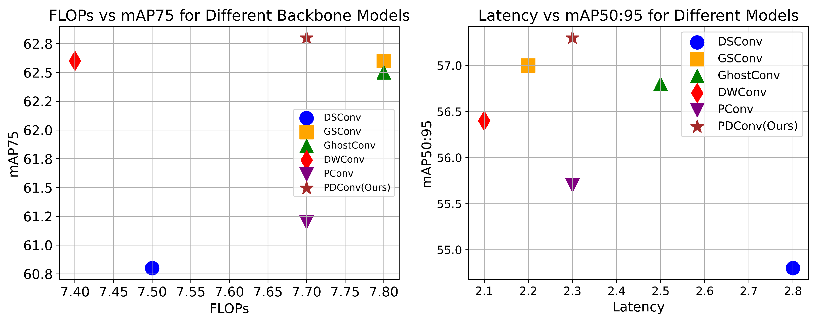
4.2. PDConv Is Low FLOPs

To demonstrate that our DPConv has low FLOPs and parameter counts, we next stacked five layers of convolutions, constructed a simple CNN network with feature maps of typical dimensions as input, and computed the FLOPs required for each layer of the convolution, the parameters, and the memory occupied by each layer. For comparison, this article did the same for the other convolutions. The results in

Table 2. The CNN network constructed after five layers of convolutional stacking has an input size of 3 × 640 × 640 and the convolutional kernel used is 3 × 3. The grouping of GConv in the first layer of the convolution is 3, and the last four layers use a grouping of 16, which is consistent with the current input channel. “Feature Map” refers to the size of the feature map, and “Memory” refers to its memory usage, where the BN layer is ignored, and the activation function layer.

Operator	Feature Map	Params	Memory (M)	FLOPs (M)
PDConv 3 × 3	16 × 320 × 320	198	75	90
	32 × 160 × 160	712	37.5	79
	64 × 80 × 80	2448	18.7	65
	128 × 40 × 40	8992	9.3	59
	256 × 20 × 20	34,368	4.7	56
	Total	46,718	145.2	349
StandrdConv 3 × 3	16 × 320 × 320	464	82.8	204
	32 × 160 × 160	4672	40.6	485
	64 × 80 × 80	18,560	20.3	478
	128 × 40 × 40	73,984	10.1	475
	256 × 20 × 20	295,424	5.1	473
	Total	393,104	158.9	2115
DWConv 3 × 3	16 × 320 × 320	94	60.9	52
	32 × 160 × 160	704	34.4	79
	64 × 80 × 80	2432	17.2	66
	128 × 40 × 40	8960	8.6	59
	256 × 20 × 20	34,304	4.3	56
	Total	46,494	125.4	312
GConv 3 × 3 (g = 16)	16 × 320 × 320	464	82.9	203
	32 × 160 × 160	352	40.1	43
	64 × 80 × 80	1280	20.3	36
	128 × 40 × 40	4864	6.9	33
	256 × 20 × 20	18,944	5.1	31
	Total	25,904	155.3	346

show that PDConv and DWConv have similar consumption in terms of Params and FLOPs; however, as mentioned earlier, DWConv, due to its characteristics, undergoes more accuracy degradation as the number of network layers deepens. While comparing StandrdConv, the number of parameters compresses more than eight times and FLOPs drop by more than six times. Although the data in the table show that GConv looks more attractive in terms of the number of parameters, the use of GConv [46] is often accompanied by an increase in the number of channels to compensate for the loss of accuracy, which undoubtedly increases the complexity of the model. As for memory, lower memory is another factor that affects inference speed due to the constraints of the memory bottleneck, but this also means that, if the memory bottleneck is sufficient enough to support the consumption of convolutions, inference speed is strongly correlated with FLOPs.

4.3. Experiment on CoCo2017

To evaluate the generalization ability of the network, this article utilized the COCO2017 dataset, a widely recognized benchmark provided by the Microsoft team for image recognition tasks. This dataset is extensively used for various computer vision tasks, including object detection, instance segmentation, and keypoint detection, due to its diverse and complex real-world scenarios.

The COCO2017 dataset consists of a training set (118,287 images), a validation set (5000 images), and a test set (40,670 images). It features annotations for 80 object categories commonly encountered in daily life, along with high-quality bounding boxes, instance masks, and keypoints. The dataset’s richness in multi-object scenes, varied resolutions, and occlusions makes it a reliable standard for assessing the performance and robustness of models in realistic settings.

This article conducted detector experiments for One Stage and Two Stage to evaluate the network performance on metrics covering mAP50, mAP75, and FLOPs. In

Table 3. Experiments were performed on the COCO2017 dataset [47]. FasterNet was chosen for the two stage target detector, using FasterNet as the baseline and replacing its convolution with our PDConv with reference to FasterNet. Twelve epochs were trained with a batch size of 16, and other training settings were not further adjusted for hyperparameters. Additionally, YOLOv8 was chosen as baseline for the single-stage target detector, the initial learning rate was set to 0.1, while the final learning rate was set to 0.01, the number of warm-up training rounds was set to 3, and 24 epochs were trained.

Backbone	mAP50	mAP75	FLOPs
Two Stage
ResNet50	55.1	36.7	253
PoolFormer-S24 [48]	59.1	39.6	233
PVT-Small [49]	60.1	40.3	238
FasterNet-S	58.1	39.7	258
FasterNet-PDConv(ours)	58.0	39.4	243
ResNet101	57.7	38.8	329
ResNeXt101-32x4d	59.4	40.2	333
PoolFormer-S36	60.1	40.0	266
PVT-Medium	61.6	42.1	295
FasterNet-M	61.5	42.3	344
FasterNet-PDConv(ours)	61.8	42.4	325
ResNeXt101-64x4d	60.6	41.3	487
PVT-Large	61.9	42.5	358
FasterNet-L	62.3	43.0	484
FasterNet-PDConv(ours)	62.0	43.1	450
One Stage
YOLOv8-S	47.2	35.8	28.7
RepVit-S	47.5	36.6	29
PDNet-S(ours)	47.6	36.9	27
YOLOv8-M	53.2	42.1	79.1
EfficientNetV2	41.8	31.2	23.1
RepVit-M	54.2	42.7	79
PDNet-M(ours)	53.5	42.4	76
YOLOv8-L	56.4	45.2	166
RepVit-L	57.1	45.8	166
HorNet	54.7	43.7	188
PDNet-L(ours)	57.5	46.3	160

, this paper reported, in detail, the results of the object detection experiments conducted on the test set.

Experimental results on the COCO2017 dataset further validate the advantages of PDConv and PDNet. Compared with other lightweight models, PDConv effectively reduces the computational complexity by reducing the computation of redundant feature maps while maintaining high performance in several accuracy metrics. For example, on the FasterNet architecture, the model using PDConv (FasterNet-PDConv) performs comparably or slightly lower than the original architecture on mAP50 and mAP75, but there is a significant reduction in FLOPs, reflecting the improvement in computational efficiency. As for the One Stage detectors in the YOLOv8 series, PDNet improves mAP50 and mAP75 while maintaining lower FLOPs, especially in the PDNet-S and PDNet-M versions, which show more obvious advantages, especially in striking an excellent balance between efficient computation and accuracy.

Specifically, in the two stage detector, the training setup follows PConv, and our PDConv is equipped with the advanced FasterNet. This article performed three comparison experiments on the three models of detectors, S, M, and L. Our FasterNet-PDConv obtained the best accuracies in the medium model backbone, reaching 61.8% and 42.4%, respectively, while FLOPs are also relatively low, reaching 61.8% and 42.4%, with 0.3% and 0.1% improvement in mAP compared to FasterNet-M mAP, respectively, and relatively low FLOPs. In the large backbone, our FasterNet-PDConv achieved the best result of 43.1% at mAP75 and had FLOPs second only to PVT-Large.

In the One Stage detector, our PDNet shows the best results in both S and L models, with PDNet-S showing 0.4% and 1.1% improvement in mAP and 1.7 G lower FLOPs compared to YOLOv8-S. In the large detector, PDNet-L outperforms YOLOv8-L by 1.1% in terms of accuracy and also has the lowest FLOPs. This definitely proves the validity of our work.

4.4. Ablation Experiment

In order to evaluate the effectiveness of the five different lightweight convolution methods, as well as to ensure the fairness of the experiments, this article conducted the experiments using the same detector YOLOv8n and uniform hyperparameters. For the PASCAL VOC test set, this article performed a comparison of the lightweight convolution methods, with evaluation criteria covering the complexity of the models as well as two accuracy metrics. For each experimental setup, the number of training rounds was 200, the number of warm-up rounds was three, and the momentum was set to 0.937. This ensured that the experiments were performed under identical conditions to improve the fairness of the comparison. For layers 3, 5 and 7 of the feature extraction network, this article introduced five lightweight convolution methods and recorded the experimental results in detail in

Table 4. Comparison of lightweight convolution methods. Includes DSConv, GSConv, Ghost Conv, DWConv, and PConv. To accommodate the network structure, PConv is upsampled and downsampled once and Latency calculations are performed under a GTX3070. The dataset used is PASCAL VOC.

Methods	FLOPs	Param	Latency	mAP75	mAP50:95
DSConv	7.5	2.7	2.8 ms	60.8	54.8
GSConv	7.8	2.8	2.2 ms	62.6	57.0
Ghost Conv	7.8	2.8	2.5 ms	62.5	56.8
DWConv	7.4	2.6	2.1 ms	62.6	56.4
PConv	7.8	2.7	2.3 ms	61.2	55.7
PDConv(Ours)	7.7	2.8	2.3 ms	62.8	57.3

. These results provide a comprehensive assessment of the performance of the different lightweight convolution methods and provide clear data support for comparing their effectiveness.

Table 4 shows that PDConv compares some popular lightweight convolutions and is equal to DWConv in Latency metrics but also that the accuracy of PDConv is superior. Moreover, the Latency consumption of DSConv and Ghost Conv to compensate for the accuracy is obvious. DWConv, the most popular lightweight convolution, has the lowest number of parameters and computations in existence, but its accuracy is slightly inferior. Although PDConv does not look the most attractive in terms of inference speed, the accuracy does reach the highest level. In fact, the pursuit of extreme speed will inevitably lead to a decrease in accuracy, and this article prefers to achieve a balance between the two. While inference speed is not strongly correlated with FLOPs and Param, DSConv, despite having relatively low FLOPs (7.5G), is actually a PWConv after DWConv, which can be limited by memory bottlenecks; indeed, our PDConv suffers from the same kind of problem, but used partially lighter operations to alleviate such problems in some ways. In order to observe the results in the table more intuitively, this article ploted the results in Figure 6.

PDConv achieves a better balance between accuracy and computational efficiency than other lightweight convolution methods (e.g., DWConv, DSConv, and GhostConv). DWConv, as a classical lightweight convolution, has the lowest computational complexity but compromises on feature extraction accuracy. Although DSConv and GhostConv improve the accuracy by increasing the Latency consumption, they still fail to effectively solve the memory bottleneck problem. PDConv solves the feature redundancy problem by introducing a dynamic channel processing mechanism, which firstly reduces the number of channels by half through 1 × 1 convolution, then extracts the deep features through DWConv while, at the same time, retaining the unprocessed channels to reduce the loss of information and finally restoring the channel information through upscaling and splicing. Finally, the channel information is recovered by upscaling and splicing. Compared with the grouping strategy of GSConv, PDConv is more flexible, which not only retains the key information but also greatly reduces the computational complexity. This design is especially suitable for deep networks, which can reduce redundancy while maintaining high computational efficiency and feature extraction capabilities.

Although the inference speed of PDConv is slightly lower than that of DWConv, its accuracy is significantly better than other methods. The computational complexity analysis shows that the FLOPs of PDConv are similar to those of DWConv, which effectively alleviates the memory bottleneck by partially lightweighting the operation and maintains the high feature expressiveness in deep networks. Experimental results show that PDConv improves accuracy while still maintaining acceptable inference efficiency, validating its superior balance between speed and accuracy. This advantage makes PDConv more competitive in practical applications.

To further validate the effectiveness of our constructed PDConv, 1×, 2×, and 3× substitutions were made to the network. The results of these experiments are reported in detail in

Table 5. The effect of different specifications of PDConv on the network, with the number of iterations set to 100 and other parameters remaining the same as above. The dataset used is PASCAL VOC.

Methods	mAP50	mAP75	mAP50:95	Param	FLOPs
PDConv 1×	72.7	58.3	53.1	2.93 M	7.9 G
PDConv 2×	73.0	59.1	53.3	2.90 M	7.8 G
PDConv 3×	72.4	59.0	53.0	2.77 M	7.7 G

. Through these experiments, this article was able to gain insight into the role of PDConv in network performance. In Table 5, this article reported the results of this experiment; 2× looks more attractive compared to 1× and 3×, but 3× is more advantageous in terms of Param and FLOPs. It is worth noting that there tend to be more redundant feature maps in the deeper structure of the network, where the use of PDConv gives better results.

In

Table 6. Ablation experiment with 100 iterations; the dataset used is PASCAL VOC.

Methods	mAP50	mAP75	mAP50:95
Baseline	72.3	58.8	52.9
Baseline+PDConv	72.7	58.3	53.1
Baseline+PDConv+PDC2f	72.7	59.0	52.9
Baseline+PDConv+PDC2f+DCN	73.8	59.2	53.9

, the ablation experiments demonstrate changes in model performance in a sequence of stepwise improvements. Starting from Baseline (A), PDConv (B), PDC2f (C) and DCN (D) were added gradually. The results show an overall gradual improvement in performance metrics as each component is added.

5. Limition and Future Work

This study introduces PDConv, a novel convolution method designed to tackle the often-overlooked problem of feature map redundancy in lightweight object detection models. By compressing redundant feature maps and leveraging an efficient network width enhancement strategy, PDConv achieves a balance between computational efficiency and accuracy, making it highly suitable for resource-constrained environments such as real-time edge applications. The experimental results on PASCAL VOC and COCO2017 datasets demonstrate its practical utility, showcasing its ability to outperform traditional methods in lightweight model design. Compared to existing approaches, PDConv offers a unique advantage in regard to minimizing computational overhead while preserving critical feature information, contributing to the ongoing advancement of lightweight architectures in computer vision.

While the results are promising, this work also highlights potential areas for further exploration. For instance, PDConv’s current design may face challenges in tasks requiring extremely fine-grained feature differentiation. However, this opens up opportunities to develop more refined variants with tailored hyperparameter configurations and enhanced structural flexibility. Additionally, while this study primarily evaluates PDConv on benchmark datasets, its adaptability to more specialized or complex tasks remains a valuable avenue for future research. These considerations do not detract from the strengths of PDConv but rather suggest pathways to further enhance its performance and applicability.

In the future, we will focus on expanding the versatility of PDConv by exploring different variants, optimizing hyperparameter configurations through advanced techniques and testing its performance in broader application domains, such as medical imaging and autonomous driving. Furthermore, incorporating complementary mechanisms, such as lightweight attention modules, may further boost its feature extraction capabilities. These improvements aim to solidify PDConv’s position as a highly effective and generalizable solution for lightweight computer vision tasks, reinforcing its practical value in both research and real-world applications.

6. Conclusions

This paper addressed the problem of feature map redundancy by proposing an innovative lightweight convolution technique named PDConv. This technique aims at efficiently eliminating redundancy with minimal impact on the ability to perform effective feature extraction. This article provided a review of the history of lightweight model development and an in-depth analysis of the value and contributions that these models bring. Subsequently, this article provided an exhaustive analysis of the complexity of PDConv and applied it to construct PDBottleNeck and PDC2f. Finally, this paper built PDNet in an extensive experimental validation and verified the effectiveness of the proposed convolutional technique and the excellent performance of the PDNet network structure on the PASCAL VOC and CoCo2017 datasets. These results further highlight the academic contributions of our approach and its potential applications in the field of lightweight deep learning models.

References

1. Howard, A.G.; Zhu, M.; Chen, B.; Kalenichenko, D.; Wang, W.; Weyand, T.; Andreetto, M.; Adam, H. MobileNets: Efficient Convolutional Neural Networks for Mobile Vision Applications. arXiv 2017, arXiv:1704.04861. [Google Scholar]
2. Howard, A.; Sandler, M.; Chen, B.; Wang, W.; Chen, L.C.; Tan, M.; Chu, G.; Vasudevan, V.; Zhu, Y.; Pang, R.; et al. Searching for MobileNetV3. In Proceedings of the 2019 IEEE/CVF International Conference on Computer Vision (ICCV), Seoul, Republic of Korea, 27 October–2 November 2019; pp. 1314–1324. [Google Scholar] [CrossRef]
3. Sandler, M.; Howard, A.; Zhu, M.; Zhmoginov, A.; Chen, L.C. MobileNetV2: Inverted Residuals and Linear Bottlenecks. In Proceedings of the 2018 IEEE/CVF Conference on Computer Vision and Pattern Recognition, Salt Lake City, UT, USA, 18–23 June 2018; pp. 4510–4520. [Google Scholar] [CrossRef]
4. Zhang, X.; Zhou, X.; Lin, M.; Sun, J. ShuffleNet: An Extremely Efficient Convolutional Neural Network for Mobile Devices. In Proceedings of the 2018 IEEE/CVF Conference on Computer Vision and Pattern Recognition, Salt Lake City, UT, USA, 18–23 June 2018; pp. 6848–6856. [Google Scholar] [CrossRef]
5. Ma, N.; Zhang, X.; Zheng, H.; Sun, J. ShuffleNet V2: Practical Guidelines for Efficient CNN Architecture Design. arXiv 2018, arXiv:1807.11164. [Google Scholar]
6. Han, K.; Wang, Y.; Tian, Q.; Guo, J.; Xu, C.; Xu, C. GhostNet: More Features From Cheap Operations. In Proceedings of the 2020 IEEE/CVF Conference on Computer Vision and Pattern Recognition (CVPR), Seattle, WA, USA, 13–19 June 2020; pp. 1577–1586. [Google Scholar] [CrossRef]
7. Chen, Y.; Fan, H.; Xu, B.; Yan, Z.; Kalantidis, Y.; Rohrbach, M.; Shuicheng, Y.; Feng, J. Drop an Octave: Reducing Spatial Redundancy in Convolutional Neural Networks With Octave Convolution. In Proceedings of the 2019 IEEE/CVF International Conference on Computer Vision (ICCV), Seoul, Republic of Korea, 27 October–2 November 2019; pp. 3434–3443. [Google Scholar] [CrossRef]
8. He, T.; Tan, J.; Zhuo, W.; Printz, M.; Chan, S.H.G. Tackling Multipath and Biased Training Data for IMU-Assisted BLE Proximity Detection. In Proceedings of the IEEE INFOCOM 2022—IEEE Conference on Computer Communications, Virtual, 2–5 May 2022; pp. 1259–1268. [Google Scholar] [CrossRef]
9. Li, Y.; Chen, Y.; Dai, X.; Chen, D.; Liu, M.; Yuan, L.; Liu, Z.; Zhang, L.; Vasconcelos, N. MicroNet: Improving Image Recognition with Extremely Low FLOPs. In Proceedings of the 2021 IEEE/CVF International Conference on Computer Vision (ICCV), Montreal, QC, Canada, 10–17 October 2021; pp. 458–467. [Google Scholar]
10. Sifre, L.; Mallat, S. Rigid-Motion Scattering for Texture Classification. arXiv 2014, arXiv:1403.1687. [Google Scholar]
11. Singh, P.; Verma, V.K.; Rai, P.; Namboodiri, V.P. HetConv: Heterogeneous Kernel-Based Convolutions for Deep CNNs. In Proceedings of the 2019 IEEE/CVF Conference on Computer Vision and Pattern Recognition (CVPR), Long Beach, CA, USA, 15–20 June 2019; pp. 4830–4839. [Google Scholar]
12. Zhang, T.; Qi, G.J.; Xiao, B.; Wang, J. Interleaved Group Convolutions for Deep Neural Networks. arXiv 2017, arXiv:1707.02725. [Google Scholar]
13. Zhuo, W.; Chiu, K.; Chen, J.; Tan, J.; Sumpena, E.; Chan, S.H.G.; Ha, S.; Lee, C.H. Semi-supervised Learning with Network Embedding on Ambient RF Signals for Geofencing Services. In Proceedings of the 2023 IEEE 39th International Conference on Data Engineering (ICDE), Anaheim, CA, USA, 3–7 April 2023; pp. 2713–2726. [Google Scholar]
14. Tan, M.; Le, Q.V. EfficientNet: Rethinking Model Scaling for Convolutional Neural Networks. arXiv 2019, arXiv:1905.11946. [Google Scholar]
15. Tan, M.; Le, Q.V. EfficientNetV2: Smaller Models and Faster Training. In Proceedings of the International Conference on Machine Learning, Virtual, 18–24 July 2021. [Google Scholar]
16. Han, K.; Wang, Y.; Zhang, Q.; Zhang, W.; Xu, C.; Zhang, T. Model Rubik’s Cube: Twisting Resolution, Depth and Width for TinyNets. arXiv 2020, arXiv:2010.14819. [Google Scholar]
17. Huang, G.; Liu, S.; Maaten, L.v.d.; Weinberger, K.Q. CondenseNet: An Efficient DenseNet Using Learned Group Convolutions. In Proceedings of the 2018 IEEE/CVF Conference on Computer Vision and Pattern Recognition, Salt Lake City, UT, USA, 18–23 June 2018; pp. 2752–2761. [Google Scholar] [CrossRef]
18. Yang, L.; Jiang, H.; Cai, R.; Wang, Y.; Song, S.; Huang, G.; Tian, Q. CondenseNet V2: Sparse Feature Reactivation for Deep Networks. In Proceedings of the 2021 IEEE/CVF Conference on Computer Vision and Pattern Recognition (CVPR), Nashville, TN, USA, 20–25 June 2021; pp. 3568–3577. [Google Scholar] [CrossRef]
19. Chen, J.; He, T.; Zhuo, W.; Ma, L.; Ha, S.; Chan, S.G. TVConv: Efficient Translation Variant Convolution for Layout-aware Visual Processing. In Proceedings of the 2022 IEEE/CVF Conference on Computer Vision and Pattern Recognition (CVPR), New Orleans, LA, USA, 18–24 June 2022; pp. 12538–12548. [Google Scholar] [CrossRef]
20. Tan, M.; Chen, B.; Pang, R.; Vasudevan, V.; Sandler, M.; Howard, A.; Le, Q.V. MnasNet: Platform-Aware Neural Architecture Search for Mobile. In Proceedings of the 2019 IEEE/CVF Conference on Computer Vision and Pattern Recognition (CVPR), Long Beach, CA, USA, 15–20 June 2019; pp. 2815–2823. [Google Scholar] [CrossRef]
21. Wu, B.; Dai, X.; Zhang, P.; Wang, Y.; Sun, F.; Wu, Y.; Tian, Y.; Vajda, P.; Jia, Y.; Keutzer, K. FBNet: Hardware-Aware Efficient ConvNet Design via Differentiable Neural Architecture Search. In Proceedings of the 2019 IEEE/CVF Conference on Computer Vision and Pattern Recognition (CVPR), Long Beach, CA, USA, 15–20 June 2019; pp. 10726–10734. [Google Scholar] [CrossRef]
22. Wan, A.; Dai, X.; Zhang, P.; He, Z.; Tian, Y.; Xie, S.; Wu, B.; Yu, M.; Xu, T.; Chen, K.; et al. FBNetV2: Differentiable Neural Architecture Search for Spatial and Channel Dimensions. In Proceedings of the 2020 IEEE/CVF Conference on Computer Vision and Pattern Recognition (CVPR), Seattle, WA, USA, 13–19 June 2020; pp. 12962–12971. [Google Scholar] [CrossRef]
23. Dai, X.; Wan, A.; Zhang, P.; Wu, B.; He, Z.; Wei, Z.; Chen, K.; Tian, Y.; Yu, M.; Vajda, P.; et al. FBNetV3: Joint Architecture-Recipe Search using Neural Acquisition Function. arXiv 2020, arXiv:2006.02049. [Google Scholar]
24. Wu, B.; Li, C.; Zhang, H.; Dai, X.; Zhang, P.; Yu, M.; Wang, J.; Lin, Y.; Vajda, P. FBNetV5: Neural Architecture Search for Multiple Tasks in One Run. arXiv 2021, arXiv:2111.10007. [Google Scholar]
25. Steiner, A.; Kolesnikov, A.; Zhai, X.; Wightman, R.; Uszkoreit, J.; Beyer, L. How to train your ViT? Data, Augmentation, and Regularization in Vision Transformers. arXiv 2021, arXiv:2106.10270. [Google Scholar]
26. Touvron, H.; Cord, M.; Douze, M.; Massa, F.; Sablayrolles, A.; J’egou, H. Training data-efficient image transformers & distillation through attention. In Proceedings of the International Conference on Machine Learning, Virtual, 13–18 July 2020. [Google Scholar]
27. Graham, B.; El-Nouby, A.; Touvron, H.; Stock, P.; Joulin, A.; Jégou, H.; Douze, M. LeViT: A Vision Transformer in ConvNet’s Clothing for Faster Inference. In Proceedings of the 2021 IEEE/CVF International Conference on Computer Vision (ICCV), Montreal, BC, Canada, 11–17 October 2021; pp. 12239–12249. [Google Scholar] [CrossRef]
28. Liu, Z.; Hu, H.; Lin, Y.; Yao, Z.; Xie, Z.; Wei, Y.; Ning, J.; Cao, Y.; Zhang, Z.; Dong, L.; et al. Swin Transformer V2: Scaling Up Capacity and Resolution. In Proceedings of the 2022 IEEE/CVF Conference on Computer Vision and Pattern Recognition (CVPR), New Orleans, LA, USA, 18–24 June 2022; pp. 11999–12009. [Google Scholar] [CrossRef]
29. Liu, Z.; Lin, Y.; Cao, Y.; Hu, H.; Wei, Y.; Zhang, Z.; Lin, S.; Guo, B. Swin Transformer: Hierarchical Vision Transformer using Shifted Windows. In Proceedings of the 2021 IEEE/CVF International Conference on Computer Vision (ICCV), Montreal, BC, Canada, 11–17 October 2021; pp. 9992–10002. [Google Scholar] [CrossRef]
30. El-Nouby, A.; Touvron, H.; Caron, M.; Bojanowski, P.; Douze, M.; Joulin, A.; Laptev, I.; Neverova, N.; Synnaeve, G.; Verbeek, J.; et al. XCiT: Cross-Covariance Image Transformers. In Proceedings of the Neural Information Processing Systems, Online, 6–14 December 2021. [Google Scholar]
31. Huang, T.; Huang, L.; You, S.; Wang, F.; Qian, C.; Xu, C. LightViT: Towards Light-Weight Convolution-Free Vision Transformers. arXiv 2022, arXiv:2207.05557. [Google Scholar]
32. Lu, J.; Yao, J.; Zhang, J.; Zhu, X.; Xu, H.; Gao, W.; Xu, C.; Xiang, T.; Zhang, L. SOFT: Softmax-free Transformer with Linear Complexity. In Proceedings of the Neural Information Processing Systems, Online, 6–14 December 2021. [Google Scholar]
33. Chen, S.; Xie, E.; Ge, C.; Liang, D.; Luo, P. CycleMLP: A MLP-like Architecture for Dense Prediction. arXiv 2021, arXiv:2107.10224. [Google Scholar] [CrossRef] [PubMed]
34. Lian, D.; Yu, Z.; Sun, X.; Gao, S. AS-MLP: An Axial Shifted MLP Architecture for Vision. arXiv 2021, arXiv:2107.08391. [Google Scholar]
35. Tolstikhin, I.O.; Houlsby, N.; Kolesnikov, A.; Beyer, L.; Zhai, X.; Unterthiner, T.; Yung, J.; Keysers, D.; Uszkoreit, J.; Lucic, M.; et al. MLP-Mixer: An all-MLP Architecture for Vision. In Proceedings of the Neural Information Processing Systems, Online, 6–14 December 2021. [Google Scholar]
36. Li, H.; Li, J.; Wei, H.; Liu, Z.; Zhan, Z.; Ren, Q. Slim-neck by GSConv: A better design paradigm of detector architectures for autonomous vehicles. arXiv 2022, arXiv:2206.02424. [Google Scholar]
37. Wang, C.Y.; Liao, H.Y.M.; Yeh, I.H.; Wu, Y.H.; Chen, P.Y.; Hsieh, J.W. CSPNet: A New Backbone that can Enhance Learning Capability of CNN. In Proceedings of the 2020 IEEE/CVF Conference on Computer Vision and Pattern Recognition Workshops (CVPRW), Seattle, WA, USA, 14–19 June 2020; pp. 1571–1580. [Google Scholar]
38. Everingham, M.; Gool, L.V.; Williams, C.K.I.; Winn, J.; Zisserman, A. The Pascal Visual Object Classes (VOC) Challenge. Int. J. Comput. Vis. 2010, 88, 303–338. [Google Scholar] [CrossRef]
39. Wang, J.; Chen, K.; Xu, R.; Liu, Z.; Loy, C.C.; Lin, D. CARAFE: Content-Aware ReAssembly of FEatures. In Proceedings of the 2019 IEEE/CVF International Conference on Computer Vision (ICCV), Seoul, Republic of Korea, 27 October–2 November 2019; pp. 3007–3016. [Google Scholar] [CrossRef]
40. Li, C.; Zhou, A.; Yao, A. Omni-Dimensional Dynamic Convolution. arXiv 2022, arXiv:2209.07947. [Google Scholar]
41. Li, D.; Hu, J.; Wang, C.; Li, X.; She, Q.; Zhu, L.; Zhang, T.; Chen, Q. Involution: Inverting the Inherence of Convolution for Visual Recognition. In Proceedings of the 2021 IEEE/CVF Conference on Computer Vision and Pattern Recognition (CVPR), Nashville, TN, USA, 20–25 June 2021; pp. 12316–12325. [Google Scholar] [CrossRef]
42. Woo, S.; Park, J.; Lee, J.Y.; Kweon, I.S. CBAM: Convolutional Block Attention Module. arXiv 2018, arXiv:1807.06521. [Google Scholar]
43. Rao, Y.; Zhao, W.; Tang, Y.; Zhou, J.; Lim, S.N.; Lu, J. HorNet: Efficient High-Order Spatial Interactions with Recursive Gated Convolutions. arXiv 2022, arXiv:2207.14284. [Google Scholar]
44. Chen, H.; Wang, Y.; Guo, J.; Tao, D. VanillaNet: The Power of Minimalism in Deep Learning. arXiv 2023, arXiv:2305.12972. [Google Scholar]
45. Wang, A.; Chen, H.; Lin, Z.; Pu, H.; Ding, G. RepViT: Revisiting Mobile CNN From ViT Perspective. arXiv 2023, arXiv:2307.09283. [Google Scholar]
46. Krizhevsky, A.; Sutskever, I.; Hinton, G.E. ImageNet classification with deep convolutional neural networks. Commun. ACM 2012, 60, 84–90. [Google Scholar] [CrossRef]
47. Lin, T.Y.; Maire, M.; Belongie, S.J.; Hays, J.; Perona, P.; Ramanan, D.; Dollár, P.; Zitnick, C.L. Microsoft COCO: Common Objects in Context. In Proceedings of the European Conference on Computer Vision, Zurich, Switzerland, 6–12 September 2014. [Google Scholar]
48. Yu, W.; Luo, M.; Zhou, P.; Si, C.; Zhou, Y.; Wang, X.; Feng, J.; Yan, S. MetaFormer is Actually What You Need for Vision. In Proceedings of the 2022 IEEE/CVF Conference on Computer Vision and Pattern Recognition (CVPR), New Orleans, LA, USA, 18–24 June 2022; pp. 10809–10819. [Google Scholar]
49. Wang, W.; Xie, E.; Li, X.; Fan, D.P.; Song, K.; Liang, D.; Lu, T.; Luo, P.; Shao, L. Pyramid Vision Transformer: A Versatile Backbone for Dense Prediction without Convolutions. In Proceedings of the 2021 IEEE/CVF International Conference on Computer Vision (ICCV), Montreal, QC, Canada, 10–17 October 2021; pp. 548–558. [Google Scholar] [CrossRef]
Figure 1. PDNet backbone and PDConv structure diagram. For a 640 × 640 colour three-channel image, it is converted into a 1024 × 20 × 20 feature map after nine processing stages. PDConv on the left, © stands for concat. C stands for channels. Four convolutions of the input feature maps are performed, and the feature maps from the first convolution are spliced over the channels with the final feature maps to form the output feature maps. It is worth noting that PDConv, as well as PDC2f, can be combined in any way.
Electronics 14 00591 g001
Figure 2. As shown in the figure, the feature maps extracted after two layers of standard convolution clearly reveal some nearly identical feature maps, which this paper refers to as redundant feature maps. These redundant feature maps often appear in certain layers of the network, especially when the convolution process is simple or repetitive. They carry highly similar information, leading to wasted computational resources and inefficiency in the model. Reducing the number of redundant feature maps not only improves computational efficiency but also avoids excessive repetition of information, thereby helping the network to better extract and learn meaningful features.
Electronics 14 00591 g002
Figure 3. The feature maps extracted after two PDConvs have reduced redundant feature maps compared to those extracted by SC and are more focused on contours rather than colour information.
Electronics 14 00591 g003
Figure 4. The PDC2f diagram: First, the input feature map is processed through a 1 × 1 convolution; then, the processed feature map undergoes a split operation and is divided into multiple parts. Next, n PDBottleneck operations are performed, with each operation refining the feature map and expanding the channels. Finally, all the processed results are fused through an add operation and the final output is obtained through a 1 × 1 convolution. n, as a hyperparameter, is typically set to 1. Additionally,  C i n  and  C o u t  denote the input channel and output channels, while  C i n  =  C o u t  is commonly used in the backbone, as it is associated with the deeper layers of the network, specifically the neck layer.
Electronics 14 00591 g004
Figure 5. The regions of interest of the model are visualised using the CARD-CAM algorithm, which captures the output features of the last layer of the backbone, the SPPF layer. Based on the gradient information, CARD-CAM generates a heat map that identifies the pixels or regions that play a key role in the model decision. A confidence threshold of 0.5 is set for this experiment to show only the parts that have a significant impact on the prediction.
Electronics 14 00591 g005
Figure 6. In order to better accommodate viewing habits, this article flipped the FLOPs and Latency axes in the charts, which allowed us to observe the data more intuitively. By adopting the charts, this article was able to more intuitively observe the attractiveness and advantages of the PDConv model.
Electronics 14 00591 g006