Abstract
Channel prediction is an effective technology to support adaptive transmission in wireless communication. To solve the difficulty of accurately predicting channel state information (CSI) due to fast time-varying characteristics, a next-generation reservoir calculation network (NGRCN) is combined with CSI, and a channel prediction method for OFDM wireless communication systems based on an adaptive reinforced reservoir learning network (adaptive RRLN) is proposed. An adaptive elastic network (adaptive EN) is used to estimate the output weight matrix to avoid ill-conditioned solutions. Therefore, the adaptive RRLN has echo and oracle properties. In addition, an adaptive singular spectral analysis (adaptive SSA) method is proposed to improve the local predictability of CSI by decomposing and reconstructing CSI to improve the fitting accuracy of the channel prediction model. In the simulation section, the OFDM wireless communication systems are constructed using IEEE802.11ah and the one-step prediction, the multi-step prediction, and the robustness test are implemented and analyzed. The simulation results show that the prediction accuracy of the adaptive RRLN can reach 3 × 10⁻⁵ and 8.36 × 10⁻⁶, which offers satisfactory prediction performance and robustness.
1. Introduction
In orthogonal frequency division multiplexing (OFDM) wireless communication systems, adaptive delay equalization [1], automatic power control [2], adaptive modulation [3], adaptive coding [4], and other adaptive transmission techniques can effectively guarantee the communication quality. The prerequisite for these adaptive transmission techniques is that the transmitter side must be accurately informed of the state information of the current communication environment, i.e., channel state information (CSI). However, due to the fast time-varying characteristics of the CSI and the feedback delay, the CSI fed back from the receiver to the transmitter side is often outdated. To ensure the effectiveness of the adaptive transmission technique, the transmitter can predict the CSI in the future based on the outdated CSI, so that the transmitter side can evaluate the quality of the future transmission environment and adjust the transmission parameters in time [5]. Therefore, channel prediction is an important technique to support adaptive transmission in OFDM wireless communication systems, and it is also one of the research hotspots in the wireless communication field.
Over the past decade, research scholars at home and abroad have conducted many studies on channel prediction techniques for OFDM wireless communication systems and have proposed many prediction methods. At present, the channel prediction methods developed by scholars can mainly be divided into the following categories: the linear prediction method [6,7,8], the parametric prediction method [9,10], and the nonlinear prediction method [11,12,13,14]. In the first category, the predicted CSI sample is estimated using the weighted sum of some past CSI samples of OFDM wireless communication systems, where the weights are estimated using tools such as auto regression (AR) [15] and the least mean squares (LMS) [16]. The main advantage of this method is that it is easy to implement; however, its prediction performance is not satisfactory to some extent [17,18]. The second category can offer a high prediction performance [10,19,20]; however, it is not suitable for a fast time-varying fading channel. In the third category, the CSI samples are learned and fitted using nonlinear tools, e.g., the neural network (NN) [21] and the support vector machine (SVM) [22], and the future CSI sample is predicted in a nonlinear learning way. In the NN model, the deep learning method is also an effect channel prediction tool, and scholars have conducted much research in this area. For instance, W. Jiang et al. introduced the time-domain channel predictor based on a deep NN model [23], and P. E. G. S. Pereira et al. proposed channel prediction technology based on a convolutional neural network (CNN) to predict all possible multipaths in OFDM communication systems, and offered some promising results with the aid of a CNN method operating in the time–frequency domain [24]. Since the related parameters of the fading channel are not needed in advance, the nonlinear channel prediction method is widely superior to the former two categories. Therefore, the nonlinear channel prediction method is the current hotspot in the field of channel prediction.
Since machine learning (ML) and artificial intelligence (AI) are continually being improved, nonlinear prediction methods are also being widely developed. One type of efficient, nonlinear learning model is the reservoir learning model, and its typical model is the echo state network (ESN) model [25]. Since the introduction of the ESN model in 2004, it has been widely used to solve time-domain sequence-prediction problems in various fields, such as meteorological predictions [26], distributed photovoltaic power predictions [27], chaotic time-domain sequence predictions [28], and so on. In 2017, Y. Zhao et al. used the ESN model to solve a channel prediction problem and concluded that the ESN can offer satisfactory channel predictions in Ricean-fading scenarios [29]. Y. He et al. further imported the l1/2-norm into the ESN model to solve ill-conditioned solutions and built a time-domain channel prediction model based on the joint ESN [30]. Based on the works of Y. He, J. Zhang et al. developed a communication networking method based on the channel prediction of the time-domain channel CSI for charging piles [31]. The above works indicate that the reservoir learning model works well for solving channel prediction problems due to the echo state property. In 2021, D. Gauthier et al. introduced a simpler reservoir learning structure, i.e., the next-generation reservoir calculation network (NGRCN), where the hidden layer is a nonlinear crossover calculation, instead of a reservoir with huge neurons [32]. Compared to the traditional ESN model, the NGRCN has many advantages, such as high accuracy, low complexity, and easy implementation [33]. Since the NGRCN was proposed, scholars have conducted many studies in various fields. For example, A. Slonopas et al. used the NGRCN to predict network traffic in order to further detect anomalous network traffic [34]. A. Haluszczynski et al. attempted to solve the problem of controlling nonlinear dynamical systems using the NGRCN [35]. A. Haluszczynski also compared the NGRCN to the traditional ESN model in Ref. [35]. The above works indicate that the NGRCN is superior to the ESN. Due to its simpler structure, the NGRCN is not suitable for the fading channel in complex communication scenarios to some extent, especially with high noise power. In addition, the NGRCN does not have the echo state property. Therefore, there is still room to improve the learning performance of the NGRCN. To the best of our knowledge, there have been no reports on channel prediction work based on the NGRCN, which motivated us to conduct related research.
Like Ref. [24], we aim to address the channel prediction issue by adopting an ML approach that efficiently predicts the fading behavior of a channel based on past-trained samples. In this study, the NGRCN is integrated with the ESN model, and the former is improved by the reservoir, and an adaptive reinforced reservoir learning network (adaptive RRLN)-based channel prediction method for OFDM wireless communication systems is proposed in this work, which is the main novelty of our paper. An adaptive singular spectral analysis (adaptive SSA) is used to decompose and reconstruct the CSI in the frequency domain at the subcarrier to improve the local predictability of the CSI and the learning and prediction capability of the adaptive RRLN model. To further improve the generalization ability of the adaptive RRLN, an adaptive elastic network (adaptive EN) is utilized to estimate the output weight matrix and solve the problem of ill-conditioned solutions to the output weight matrix in the NGRCN. Therefore, the adaptive RRLN has the echo state property and oracle property, which enables it to fit the CSI with high accuracy and offer good prediction performances for OFDM wireless communication systems. The main contributions of this paper are as follows:
- (1)
- Based on the ESN model and the NGRCN model, the channel prediction model based on the adaptive RRLN is proposed for OFDM wireless communication systems in detail, including the output weight matrix estimation method, i.e., the adaptive EN and the local predictability enhancement method for CSI, i.e., the adaptive SSA.
- (2)
- Extensive evaluations (i.e., computational complexity analysis, one-step prediction, multi-step prediction, and the robust prediction test) are presented and discussed in this paper.
2. Related Theory
2.1. Channel-Estimation Technique for OFDM Wireless Communication Systems
Typical OFDM wireless communication systems usually consist of a transmitter, a receiver, and some intermediate data-processing devices. In OFDM wireless communication systems, the data source at the transmitter is successively sent to the receiving antenna through the transmitting antenna after forward error correction coding, bit interleaving, constellation mapping, serial-to-parallel conversion, an inverse fast Fourier transformation (IFFT), the addition of a cyclic prefix, and digital-to-analog conversion. In this process, the wireless RF signal undergoes decay after experiencing the wireless channel. Therefore, the receiver needs to reduce the BER through channel equalization and FEC decoding after receiving the wireless RF signal [36].
We assume that the CSI at the subcarriers of the OFDM system is invariant or slow-varying over a frame of time; in this case, the frequency-domain signal at the k-th subcarrier on the i-th OFDM symbol in the receiver can be expressed as follows:
where denotes the n-th time-domain data-sampling point of the i-th complex baseband, and is the total number of subcarriers per OFDM symbol. Therefore, the channel state information at the k-th subcarrier of the i-th OFDM symbol can be estimated by the least squares method:
where , , and denote the transmit signal, the actual CSI, and the estimation noise on the k-th subcarrier of the i-th OFDM symbol, respectively. is usually modeled as Gaussian white noise, with a mean of 0 and a variance of .
2.2. Next-Generation Reservoir Calculation Network
Based on Refs. [25,32], the structure of the ESN is shown in Figure 1 and that of the NGRCN is shown in Figure 2.
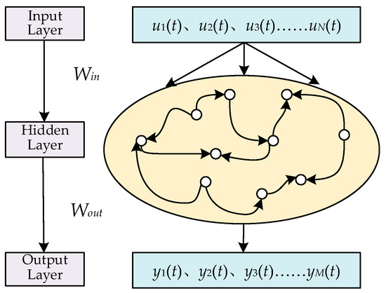
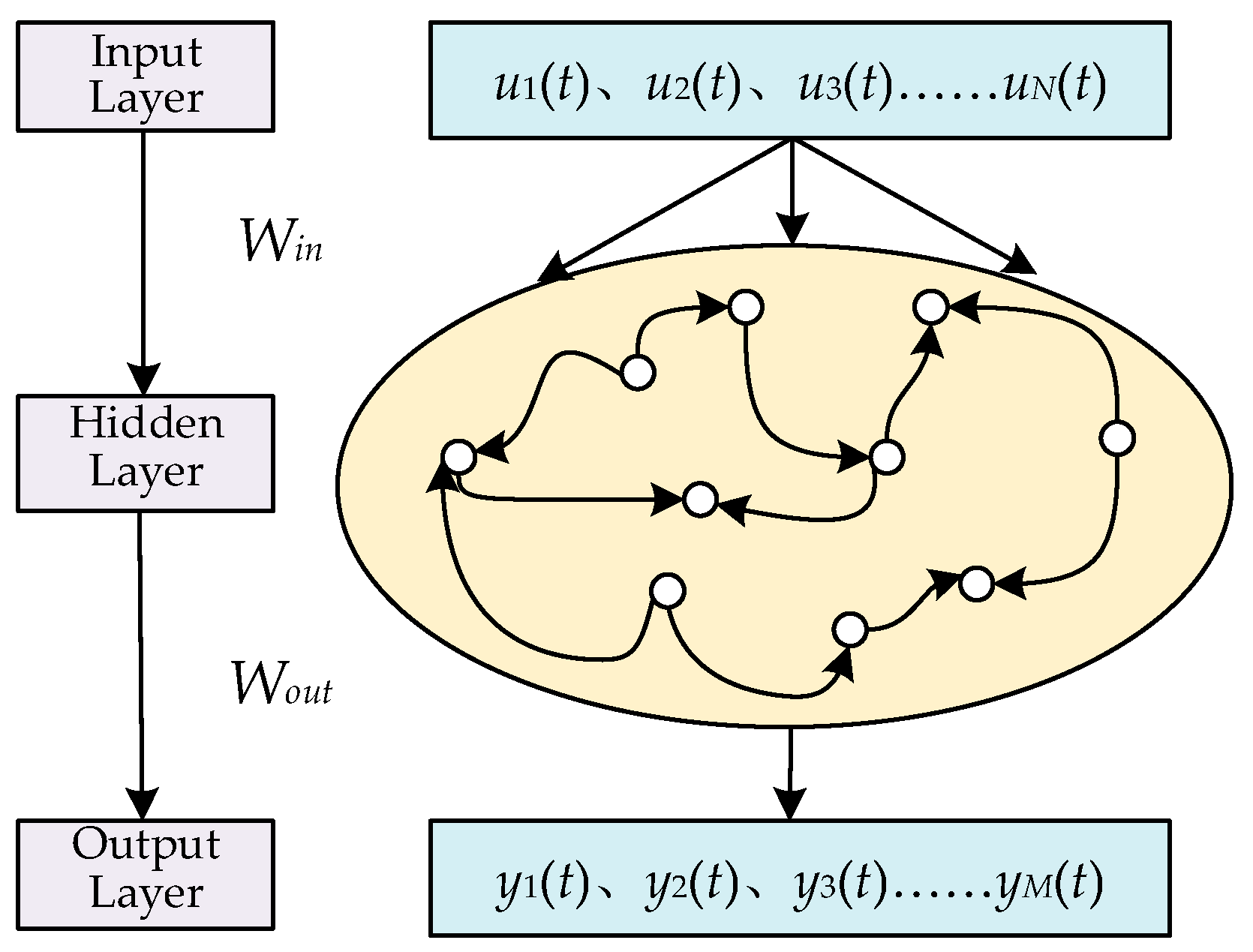
Figure 1.
The typical structure of the ESN.
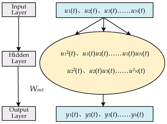
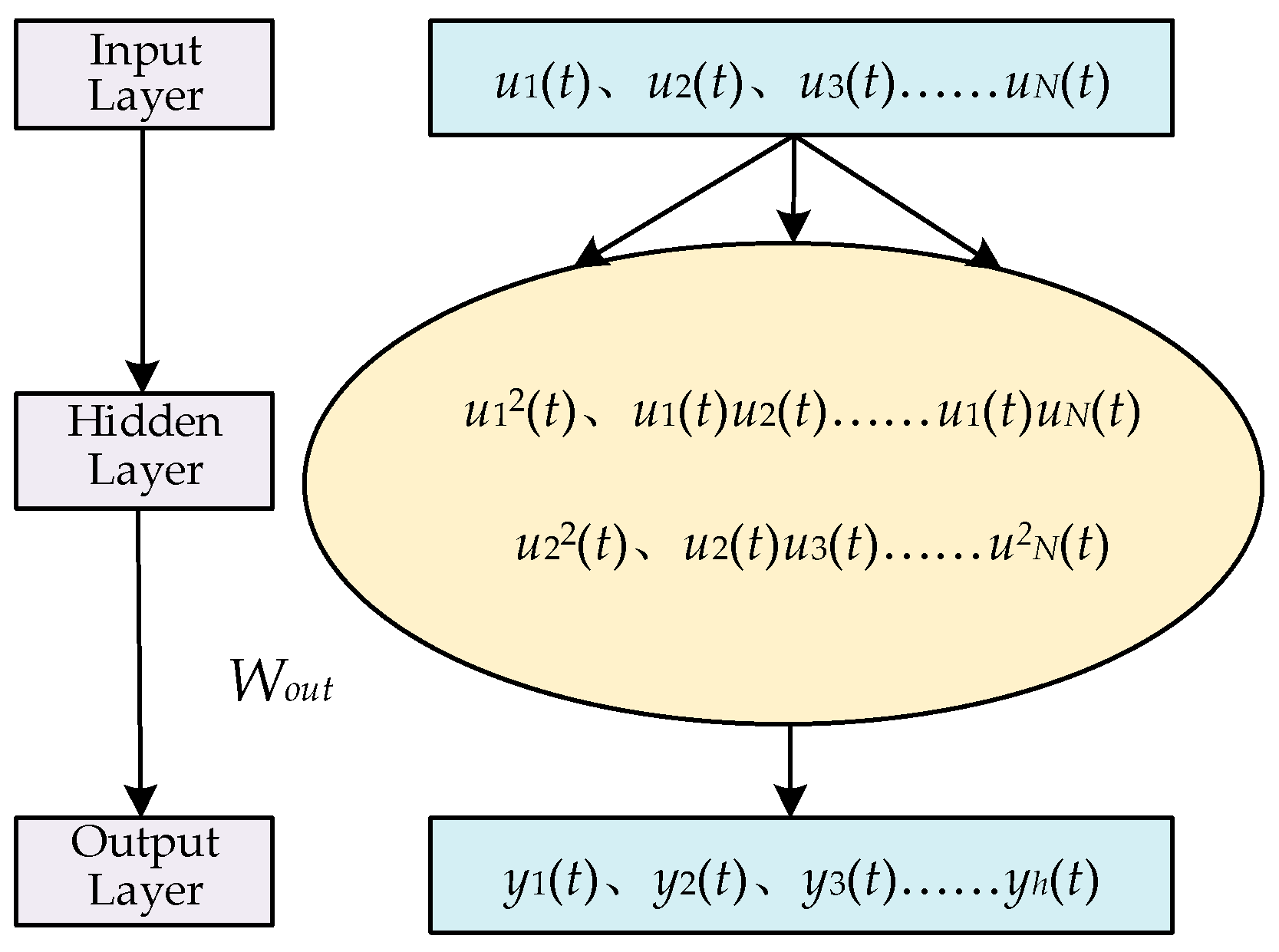
Figure 2.
The typical structure of the NGRCN.
In Figure 1, the ESN model has the reservoir; therefore, the output matrix of the reservoir for the t-th input data point is
where is the balance coefficient of the reservoir and is the hyperbolic tangent function, i.e., the activation function of the reservoir; is the scaling factor of the reservoir. is the input weight matrix and is the internal connection matrix of the reservoir, with a sparsity of SD. and are the neuron number of the input layer and the reservoir, respectively.
As can be seen from Figure 2, the NGRCN interactively multiplies the input layer data in the hidden layer, instead of the reservoir of the ESN. Therefore, when the input data are input, the output matrix of the hidden layer in the NGRCN is
where , , and are the constant part, the linear part, and the nonlinear part, respectively, and their expressions are , , and . is the n-th data point of the t-th input matrix of the NGRCN, , where denotes the input number in the training phase. denotes the transpose calculation of the matrix. Due to the linear part and the nonlinear part, the hidden layer is an equivalently powerful universal approximator and shows comparable performance to that of the standard reservoir [32].
Therefore, the output matrix can be estimated as follows:
where is the target matrix in the training process.
3. Channel Prediction Method Based on the Adaptive RRLN
3.1. Overall Calculation Methodology
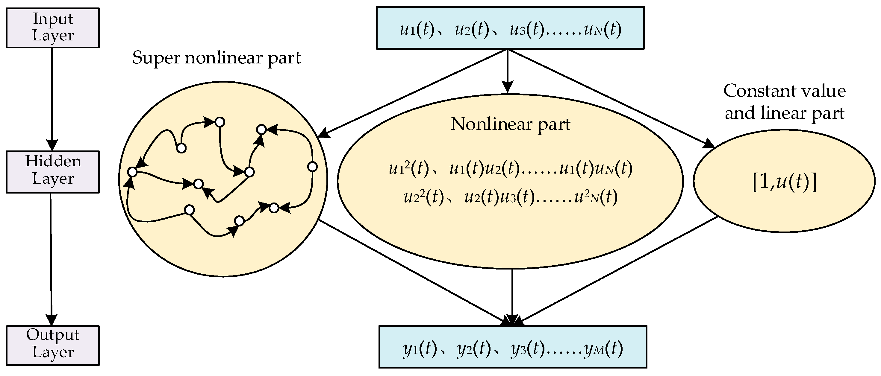
The next-generation reservoir learning network has the advantages of high accuracy, low complexity, and easy implementation but does not have the echo state property. Therefore, this research combined the savings pool with the next-generation reservoir learning network and proposed an adaptive reinforced reservoir learning network architecture, as shown in Figure 3.
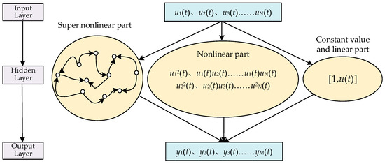
Figure 3.
The structure of the adaptive RRLN in this research.
The adaptive RRLN contains an input layer, a hidden layer, and an output layer. The hidden layer includes the constant part, the linear part, the nonlinear part, and the super nonlinear part. Therefore, by cross-calculation, the constant part, the linear part, and the nonlinear part are inherited from the NGRCN, and by importing the reservoir, the super nonlinear part with echo state property is also imported. Therefore, the adaptive RRLN has a high learning performance.
For the CSI of the k-th subcarrier of OFDM wireless communication systems, the training and prediction process can be expressed as follows:
where and are the t-th input matrix and the corresponding target matrix in the adaptive reinforced reservoir learning network, respectively; , where is the total number of input data points in the training phase. Then, the t-th output matrix of the hidden layer can be expressed as follows:
where 1 is the constant value part and denotes the linear part. denotes the nonlinear part and denotes the super-nonlinear part. Their respective expressions are as follows:
where is the balance coefficient of the reservoir; is the hyperbolic tangent function, i.e., the activation function of the reservoir; is the scaling factor of the reservoir; is the input weight matrix; and is the internal connection matrix of the reservoir with sparsity SD. When , Equation (8) can be rewritten as
In the output layer, the output weight matrix about and is estimated using the adaptive EN. When the estimated output weight matrix is obtained, the adaptive RRLN model is forward-computed to predict the CSI of OFDM wireless communication systems. The detailed training process of the adaptive RRLN in this paper is shown in Algorithm 1.
| Algorithm 1: The training process of the adaptive RRLN. |
| Input: Neuron number in the input layer , neuron number in reservoir , spectral radius , balance coefficient , scaling factor and sparse degree SD, input matrix , output matrix , the total prediction step h, and regularization coefficients and . Output: Well-trained adaptive RRLN. |
| Step 1: Optimize using an adaptive SSA; Step 2: Generate in a certain range; Step 3: Calculate using Equation (7); Step 4: Calculate using Equation (8); Step 5: Obtain using Equation (6); Step 6: Estimate the output weight matrix using adaptive EN; Step 7: Output the well-trained adaptive RRLN model. |
3.2. Estimation of Output Weight Matrix Using Adaptive EN
Since the hidden layer contains a constant value part, a linear part, a nonlinear part, and a super nonlinear part, the output matrix has a large matrix row size, and solving the output weight matrix using the least squares method would lead to ill-condition solutions. To output the weight matrix and avoid ill-conditioned solutions, we used the norm and the norm to construct the adaptive elastic network in this research:
where denotes the output weight matrix corresponding to the j-th-step prediction corresponding to the output weight matrix, and and are regularization parameters for the norm and the norm, respectively. is the adaptive factor for the j-th-step prediction corresponding to the adaptive factor of the output weight matrix. and are confirmed by the tenfold cross-verification method [37] or the experience method.
As shown in Equation (11), the adaptive elastic network contains three parts: the output matrix of the hidden layer, the output weight matrix , and the target output matrix for the training phase. The least squares calculation concerns the output weight matrix of the norm and adaptive norm. The first part preserves the output matrices and , and the second part constrains the amplitude of the output weight matrix. Then, the third part, with the adaptive factor and the estimated output weight matrix , offers the oracle property to avoid producing ill-conditioned solutions [30,38,39,40].
Based on the above elaboration, the above Equation (11) can be further rewritten as follows:
Therefore, Equation (11) can be converted to solve the j-th step to predict the loss function, with , where h is the total prediction step number. For the j-th-step prediction, Equation (12) has the following derivation:
where
where is calculated using the following equation:
where is estimated using the least squares method for the j-th-step prediction output weight matrix. Therefore, the process of solving can be transformed into the process of solving the norm about , where is the unit matrix. When is obtained, can be calculated using the following formula:
Therefore, the output weight matrix of Equation (11) can be expressed as follows:
Equation (13) can be solved using many methods, such as the Newton method (NM) [41], quasi-Newton method (QNM) [42], or least angle regression (LARS) [43]. LARS avoids the problem of no derivation in the QNM; therefore, we used the LARS method to solve Equation (13) about the norm problem of in this work.
The pseudo-code implementation of solving the output weight matrix is shown in Algorithm 2.
| Algorithm 2: Output weight matrix process using adaptive EN. |
| Input: The output matrix of the hidden layer , the output matrix of the output layer , the total prediction step h, and the regularization coefficients and . Output: Output weight matrix . |
| For : Step 1: Calculate using Equation (14); Step 2: Calculate using Equation (15); Step 3: Calculate using Equation (16); Step 4: Solve Equation (13) using LARS to obtain ; End Step 5: Output the weight matrix using Equation (18). |
3.3. Local Predictability Enhancement Method Using Adaptive SSA
In the adaptive RRLN, the hidden layer has the linear part and the nonlinear part, i.e., the direct input and the cross-multiplication operation input. To improve the generalization ability of the channel prediction model, we used the decomposition and reconstruction of CSI to improve its local predictable performance in this work through adaptive SSA.
For OFDM wireless communication systems, the trace matrix for the CSI’s of the k-th subcarrier is as follows:
where , is the number of sampling points in the singular-spectrum analysis phase and . is the window length for the adaptive singular-spectrum analysis. Generally, . Therefore, singular-value decomposition (SVD) in a standard singular-spectrum analysis is time-consuming. In this study, standard SVD is replaced with random SVD to improve the decomposition calculation rate:
where , , and denote the left singular matrix, singular matrix, and right singular matrix, respectively. is the internal matrix, and the expression is
where is the matrix’s orthogonalization calculation; is the random mapping matrix in the random singular-value decomposition; and is the rank of the trace matrix . Using Equation (21), the synthesis matrix can be obtained from the product of the singular matrix of the n-th singular value, and the product of the n-th column of the left singular matrix and the n-th row of the right singular matrix is obtained.
Therefore, the p-th of the n-th part of the channel state information can be obtained through an anti-angle averaging calculation using the random singular-value decomposition.
where denotes the synthesis matrix of the m-th row and the -th column. Therefore, the k-th channel state information of the subcarrier is decomposed into some parts, i.e., , . Through the following equation, the k-th channel state information of the subcarrier can be reconstructed using the sum of the previous decomposition parts:
where is the reorganization number, which determines the efficacy of adaptive SSA. Therefore, this value can be determined using the following equation in this work:
where is the upper rounding calculation, is the sigmoid function, and is the signal-to-noise ratio (SNR) of the CSI. In summary, this research achieved the adaptive enhancement of the local predictability performance of CSI by introducing the SNR of the current CSI into the singular-spectrum analysis calculation. The pseudo-code implementation process of the adaptive SSA is shown in Algorithm 3.
| Algorithm 3: The calculation process of the adaptive RRLN. |
| Input: The channel state information ; ; the window length ; the SNR . Output: . |
| Step 1: Randomly generate the mapping matrix ; Step 2: Obtain using Equation (20); Step 3: Obtain using Equation (22); Step 4: Calculate , , and using Equation (21); Step 5: Calculate using Equation (23); Step 6: Determine using Equation (25); Step 7: Calculate using Equation (24). |
3.4. Calculation Complexity Analysis
The calculation complexity is an important indicator for the channel prediction model. In this section, the calculation complexity of the adaptive RRLN is discussed and analyzed.
In the adaptive SSA, the calculation complexity of calculating orthogonal basis matrices, the random singular-value decomposition, and the anti-angle averaging (using Equation (21), Equation (22), and Equation (23)) are, respectively, , and . In the training stage of the adaptive reinforced reservoir learning network, the calculational complexity of the nonlinear part calculated using Equation (8) is , and the calculational complexity of the super nonlinear part calculated using Equation (9) is . Therefore, the calculation complexity for producing the hidden layer output matrix is . In the output layer, the calculation complexity of estimated using the adaptive EN is , where is the iteration number when estimating the output weight matrix of the j-th-step prediction using the LARS method. In the forward prediction stage, the calculation complexity of the nonlinear part calculated using Equation (8) is and the calculation complexity of the nonlinear part calculated using Equation (10) is . The calculation complexity of the hidden layer output matrix is . In the output prediction process, the calculation complexity of the output layer is . The computational complexity of the training process (CC-TrPr) and the prediction process (CC-PePr) for some comparable channel prediction models, i.e., AR [15], support vector machine (SVM) [22], least squares support vector machine (LS-SVM) [44], basic ESN (B-ESN) [25], the NGRCN with ridge regularization (R-NGRCN) [39], and the NGRCN with lasso regularization (L-NGRCN) [40], are shown in Table 1. Therefore, the AR model is solved using the Yule–Walker method, the SVM is implemented using Libsvm [45], and, like the adaptive EN, the L-NGRCN is solved using the LARS in our work. As we can see, the AR model has the lowest computational complexity, while the adaptive RRN has unignored calculation complexity. Therefore, it is necessary to appropriately reduce the neuron number of the input layer, the neuron number of the reservoir, the convergence accuracy, and the iteration number of the LARS for a tradeoff between the calculation complexity and the prediction performance of the system model.

Table 1.
Computational complexities of some comparable channel prediction models.
4. Simulation and Discussion
4.1. Parameter Settings
As a sub-1GHz network, the IEEE802.11ah is widely used in the power Internet of Things (IOTIPS). Compared to traditional wireless local area networks (WLANs), e.g., Bluetooth and WIFI, IEEE802.11ah can reach a wider range. Therefore, to evaluate the channel prediction performance, OFDM wireless communication systems are constructed based on the IEEE802.11ah described in this paper, the delay multipath number is set to five, and their powers and delays are [0, −2.7, −3.4, −10.3, −1.5] dB and [0, 1.5, 3.5, 5.5, 7] µs, respectively. Other relevant parameters are shown in Table 2. It should be noted that the proposed adaptive RRN is also suitable for other WLANs, not only the IEEE802.11ah in this work.
Table 2.
OFDM wireless communication systems based on IEEE802.11ah.
In this section, the OFDM systems are estimated using the least squares method to obtain the CSI at the subcarriers. Thereinto, the CSI of the first subcarrier of 8000 OFDM symbols is used to train the channel prediction model, and the CSI of the next 1000 OFDM symbols is used to test the channel prediction performance. To evaluate the effectiveness of the channel prediction method, the following indicators are considered: the mean absolute error (MAE), the root mean square error (RMSE), the normalized root mean square error (NRMSE), the symmetric mean absolute percentage error (SMAPE), the mean absolute percentage error (MAPE), the weight range of the output weight matrix (WR-OWM), and the sparse degree of the output weight matrix (SD-OWM). Among them, the MAE, RMSE, NRMSE, SMAPE, and MAPE indicate the prediction performance of the channel prediction model. The output matrix weight range and output weight matrix sparsity indicate the generalization and sparsity capabilities of the channel prediction model [46].
4.2. One-Step Prediction Analysis
In the one-step prediction test, the parameters of the adaptive RRLN are shown in Table 3. The related prediction curves are shown in Figure 4, and the related prediction results are shown in Table 4 and Table 5.
Table 3.
Parameters of the adaptive RRLN in one-step prediction.
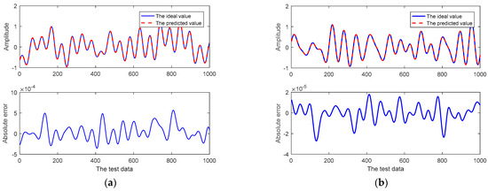
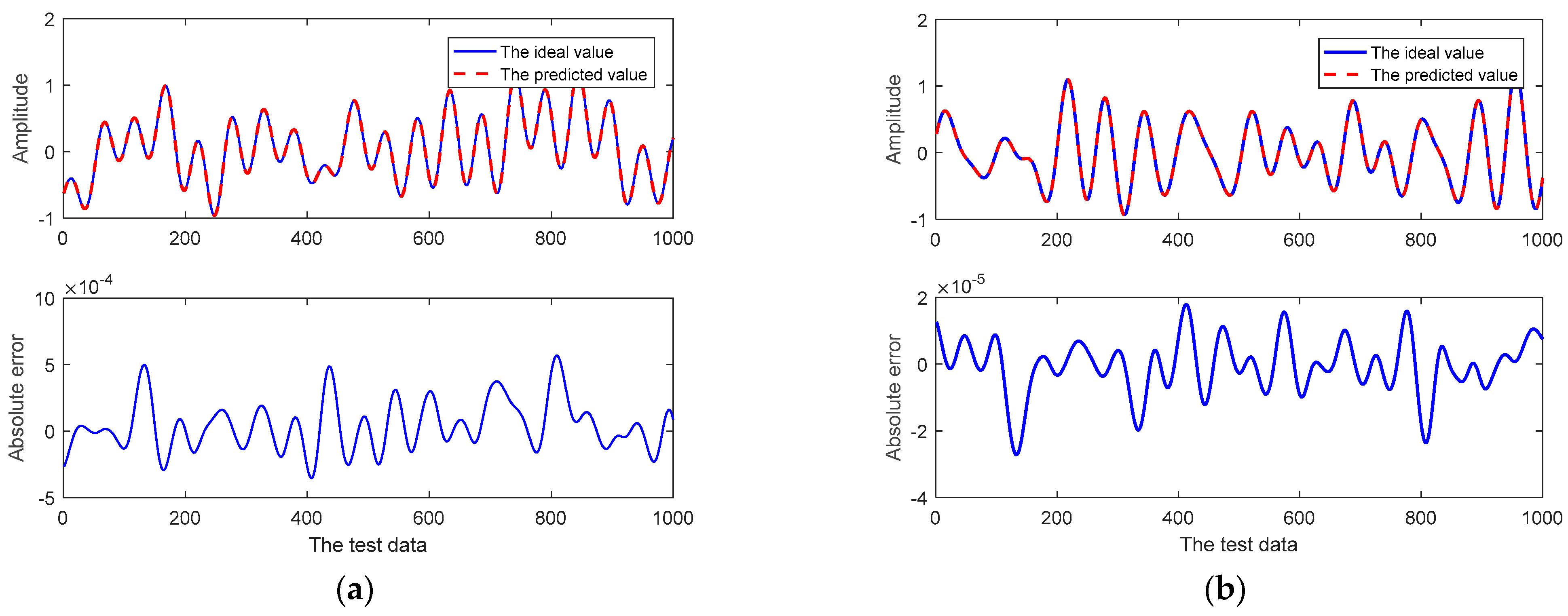
Figure 4.
The related curves of the one-step prediction of the CSI at the 1st subcarrier using the proposed prediction method: (a) the real component; (b) the imaginary component.
Table 4.
The one-step prediction results for the real component of the CSI at the 1st subcarrier.
Table 5.
The one-step prediction results for the imaginary component of the CSI at the 1st subcarrier.
As shown in Figure 4a, the adaptive RRLN offers a high fitting degree between the prediction curve and the actual curve for the real component of the CSI at the first subcarrier, and the maximum prediction error is only 5 × 10⁻⁴. Like the real component of the CSI at the first subcarrier, the prediction curve of the adaptive RRLN in this research for the imaginary part of the CSI at the first subcarrier has a higher fitting degree to the actual curve, and the maximum prediction error is only 3 × 10⁻⁴, as shown in Figure 4b.
The one-step prediction results of comparable models are given in Table 4 and Table 5. In particular, their relevant parameters are as follows. The real component: (1) AR: the order is 30; (2) SVM: and are, respectively, 22 and 0.001, and the convergence accuracy is set to 1 × 10⁻¹⁰; (3) LS-SVM: and are 500 and 151, respectively; (4) B-ESN: the input neuron number is 30, the neuron number of the reservoir is 200, its sparse degree is 0.05, its spectral radius is 0.09, the balance coefficient is 1, and the scaling factor is 0.01; (5) R-NGRCN: the input neuron number is 30 and the ridge regularization factor is 1 × 10⁻⁵; and (6) L-NGRCN: the input neuron number is 30 and the lasso regularization factor is 1 × 10⁻⁵.
The imaginary component: (1) AR: the order is 30; (2) SVM: and are 25 and 0.005, respectively, and the convergence accuracy is set to 1 × 10⁻¹⁰; (3) LS-SVM: and are, respectively, 100 and 152; (4) B-ESN: the input neuron number is 30, the neuron number of the reservoir is 200, its sparsity degree is 0.05, the spectral radius is 0.09, the balance coefficient is 1, and the scaling factor is 0.01; (5) R-NGRCN: the input neuron number is 30 and the ridge regularization factor is 1 × 10⁻⁵; and (6) L-NGRCN: the input neuron number is 30 and the lasso regularization factor is 1 × 10⁻⁵.
As shown in Table 4, for the real component of the CSI at the first subcarrier, the AR method performed the worst in terms of the relevant indicators, i.e., the MAE, RMSE, NRMSE, SMAPE, and MAPE were only 1.51 × 10⁻³, 1.89 × 10⁻³, 3.94 × 10⁻³, 1.65 × 10⁻² and 4.08 × 10⁻². The LS-SVM method had a better prediction performance than the SVM method, but all of them were worse than the predicted performance of the R-NGRCN. In addition, the output weight matrices of the AR method, LS-SVM method, SVM, and R-NGRCN are not sparse. The ranges of the output weight matrices of the B-ESN, R-NGRCN, L-NGRCN, and this study’s method are relatively close. The sparsity of the output weight matrix of the L-NGRCN method is 1.2889%, but the prediction performance is not as good as that of the adaptive RRLN in this work. Table 5 shows that, for the imaginary component of the CSI at the first subcarrier, the prediction performance of the AR method is still poor, and the prediction performance of this study’s method is the best. The ranges of the output weight matrices of the B-ESN, R-NGRCN, L-NGRCN, and adaptive RRLN are relatively close. The sparsity of the output weight matrix of the adaptive RRLN is 4.33%, which is closer to the sparsity of the output weight matrix of the L-NGRCN. As seen in Table 4 and Table 5, the adaptive RRLN has good channel prediction performance, a good output matrix weight range, and an average sparsity.
4.3. Multi-Step Prediction
Based on the one-step prediction in Section 4.1, this research conducts a multi-step prediction performance evaluation of the channel prediction models. The parameters are consistent with those used for one-step prediction. The multi-step prediction curves are shown in Figure 5.
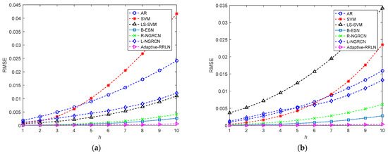
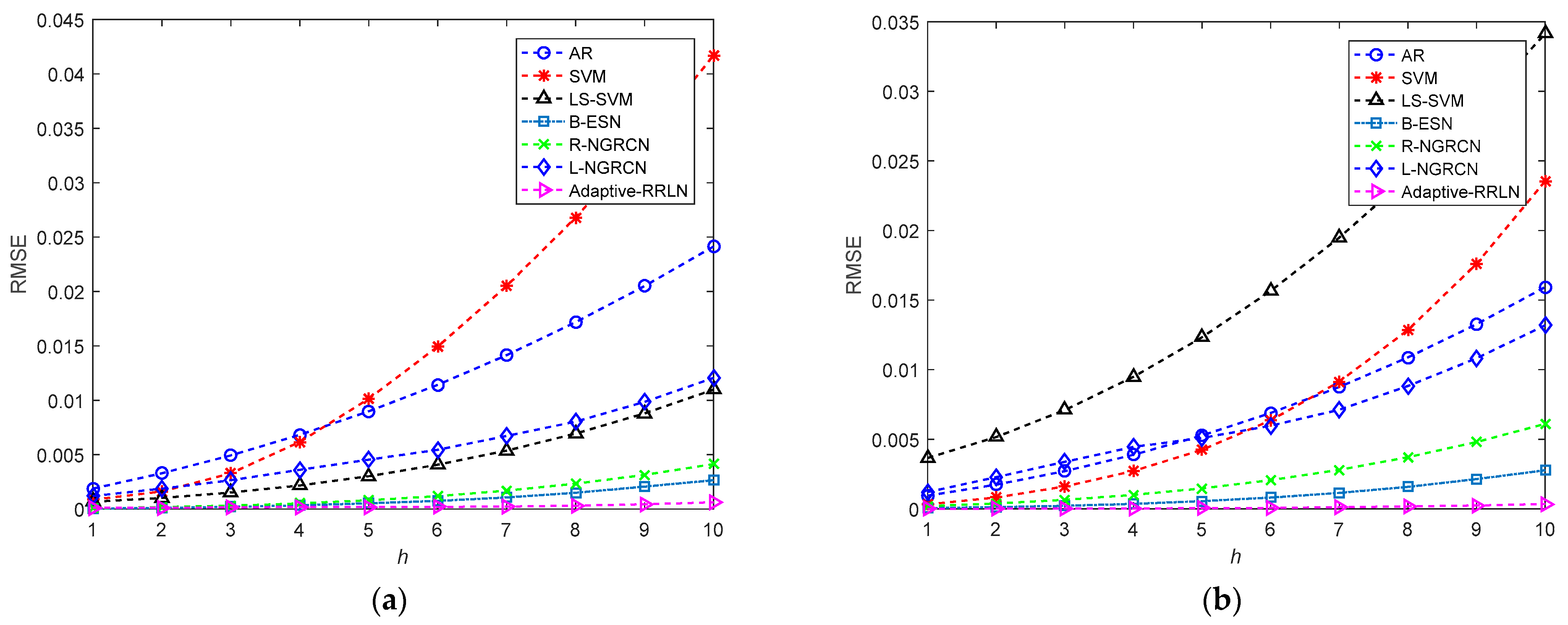
Figure 5.
The curves of the multi-step prediction of the CSI at the first subcarrier: (a) the real component; (b) the imaginary component.
As we can see from Figure 5a, as the number of prediction steps increases, the prediction error and RMSE of all the channel models also increase gradually. The channel prediction performance of the AR method is the worst when the number of prediction steps is small. The prediction performance of this study’s method and the B-ESN model is similar, and both of them outperform the SVM, LS-SVM, R-NGRCN, and L-NGRCN models. When the number of prediction steps increases, the SVM model has the worst prediction performance, whereas the method in this study still maintains very good prediction results. For example, the prediction results of AR, SVM, LS-SVM, B-ESN, R-NGRCN, and L-NGRCN at the ninth prediction step and those of the adaptive RRLN are 0.02051, 0.03387, 0.0088, 0.002068, 0.00315, 0.00985 and 4.454 × 10⁻⁴, respectively. As shown in Figure 5b, the prediction performance of the channel prediction models becomes progressively worse as the number of prediction steps increases. When the prediction step number is small, the worst-performing channel prediction is made by the LS-SVM model, followed by B-ESN, AR, SVM, R-NGRCN, and the adaptive RRLN. When the prediction step number continues to increase, i.e., when the step number is more than 7, the predicted performance of the LS-SVM model still performs the worst, followed by SVM, AR, L-NGRCN, R-NGRCN, B-ESN, and the adaptive RRLN. Therefore, for the imaginary component of the CSI at the first subcarrier, the adaptive RRLN has good multi-step prediction performance.
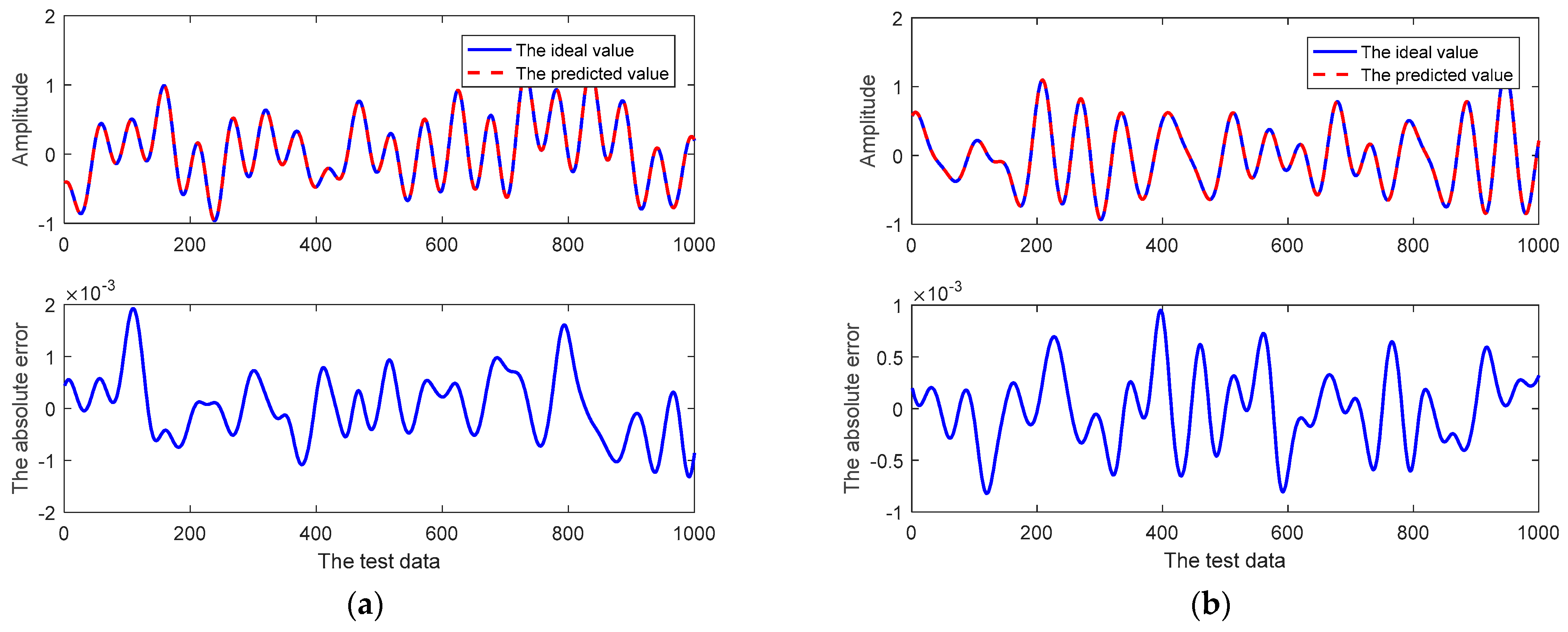
In addition, for the real component and imaginary component of the CSI at the first subcarrier, the related prediction curves of the 10th-step prediction of the adaptive RRLN are shown in Figure 6. As can be seen in Figure 6, the channel prediction curves of the adaptive RRLN still fit the ideal curves very well, with a maximum absolute error of only 2 × 10⁻³ for the real component and 1 × 10⁻³ for the imaginary component. The relevant prediction results for the 10th-step prediction are shown in Table 6 and Table 7.
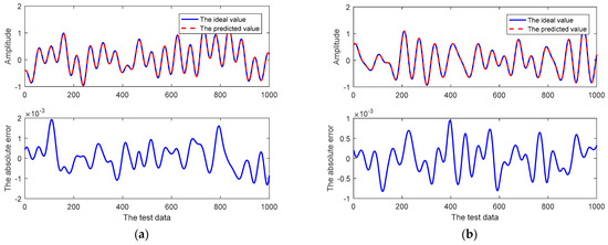
Figure 6.
The curves of the 10th step prediction of the CSI at the 1st subcarrier using the proposed prediction method: (a) the real component; (b) the imaginary component.
Table 6.
The 10th-step prediction results for the real component of the CSI at the 1st subcarrier.
Table 7.
The 10th-step prediction results for the imaginary component of the CSI at the 1st subcarrier.
As we can see from Table 6, the 10th-step prediction results of all the channel prediction models are similar to the 1-step predictions for the real component of the CSI, and the adaptive RRLN in this work is superior to the other evaluation models in terms of the MAE, RMSE, NRMSE, SMAPE, and MAPE. For the output matrix weight range, the weight range of the adaptive RRLN is larger than that of other models, but the output weight matrices of the B-ESN and R-NGRCN models are not sparse, and the sparsity of the output weight matrix of the adaptive RRLN is only 7.41%, which is superior to that of the L-NGRCN. Therefore, the adaptive RRLN has a good prediction performance for the real component of the CSI when the prediction step is 10. For the imaginary part of the CSI, the related prediction results are similar to Table 6, and we will not analyze or discuss these in detail any further.
4.4. Robust Prediction Test
To further evaluate the generalization ability and prediction performance of the channel model, a robust test of the channel prediction model is given in this section. The relevant parameters of the adaptive RRLN are shown in Table 8. Other relevant prediction model parameters are as follows: the real component: (1) AR: the order is 30; (2) SVM: and are, respectively, 25 and 0.004, and the convergence accuracy is set to 1 × 10⁻³; (3) LS-SVM: and are 5 and 12, respectively; (4) B-ESN: the input neuron number is 30, the neuron number of the reservoir is 200, its sparsity degree is 0.05, its spectral radius is 0.09, the balance coefficient is 1, and the scaling factor is 0.01; (5) R-NGRCN: the input neuron number is 30 and the ridge regularization factor is 1 × 10⁻⁴; and (6) L-NGRCN: the input neuron number is 30 and the lasso regularization factor is 1 × 10⁻⁴. The imaginary component: (1) AR: the order is 30; (2) SVM: and are, respectively, 20 and 0.1, and the convergence accuracy is set to 1 × 10⁻³; (3) LS-SVM: and are 124 and 25, respectively; (4) B-ESN: the input neuron number is 30, the neuron number of the reservoir is 200, its sparsity degree is 0.05, its spectral radius is 0.09, the balance coefficient is 1, and the scaling factor is 0.01; (5) R-NGRCN: the input neuron number is 30 and the ridge regularization factor is 1 × 10⁻⁴; and (6) L-NGRCN: the input neuron number is 30 and the lasso regularization factor is 4 × 10⁻⁴.
Table 8.
Parameters of the adaptive RRLN in the robust prediction test.
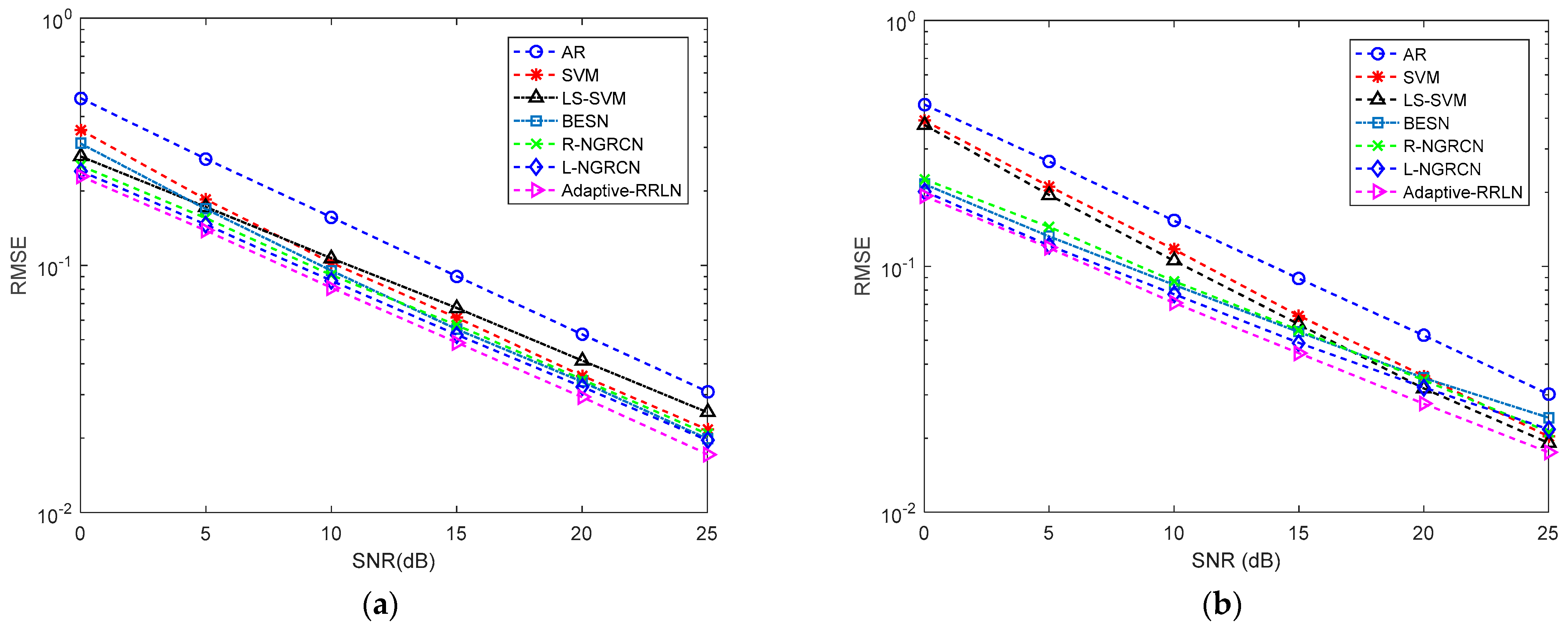
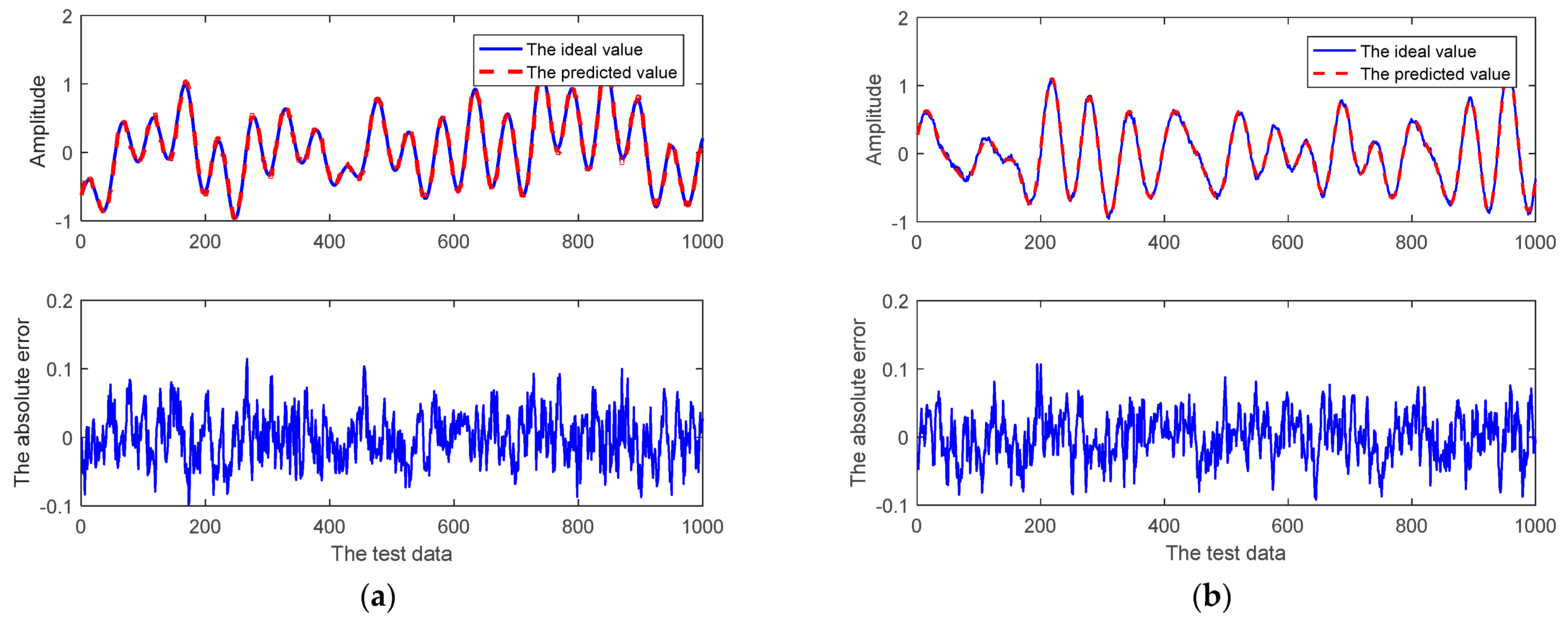
The prediction results of the given channel prediction models for the CSI at the first subcarrier for the real component and imaginary component at different SNRs are shown in Figure 7. As we can see, the prediction accuracy of all channel prediction models gradually increases when the SNR gradually increases. The AR method performs the worst, while the method of the adaptive RRLN performs the best at different SNRs. In Figure 7a, the RMSE of the adaptive RRLN is only 0.01722, while the RMSE of the AR method is 0.03087 when the SNR is 25 dB. In Figure 7b, the RMSE of the adaptive RRLN is only 0.01753, while the RMSE of the AR is 0.0302 when the SNR is 25 dB. Figure 8 shows the relevant prediction curves of the adaptive RRLN in the robustness test when the SNR is 20 dB. It can be seen that the prediction curves of the adaptive RRLN fit well with the ideal curves, and the maximum absolute error for the real component and imaginary component is only 0.1. In summary, the adaptive RRLN has a robust performance.
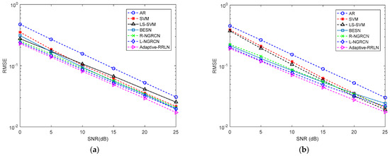
Figure 7.
The prediction performances of the CSI at the subcarrier by comparable prediction methods under different SNRs: (a) the real component; (b) the imaginary component.
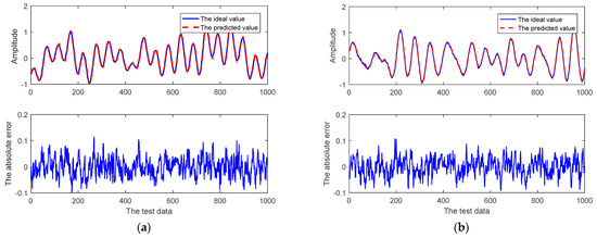
Figure 8.
The prediction performances of the CSI at the subcarrier by comparable prediction methods when SNR is 20 dB: (a) the real component; (b) the imaginary component.
5. Conclusions
In this work, we mainly focus on the channel prediction of the CSI of OFDM wireless communication systems and introduce a channel prediction method based on the adaptive RRLN by combining it with the next-generation reservoir calculation learning network. Through one-step prediction, multi-step prediction, and a robust prediction test, the following conclusions are given: (1) For the real component and imaginary component of the CSI at the first subcarrier, the one-step prediction performance of the SVM method and LS-SVM are different. For the real component, the LS-SVM is superior to the SVM, and for the imaginary component, the SVM is superior to the LS-SVM. The adaptive RRLN in this work has a good one-step prediction performance, and the RMSE can reach 3 × 10⁻⁵ and 8.36 × 10⁻⁶. (2) In multi-step prediction, the SVM and LS-SVM methods similarly show different trends. However, the adaptive RRLN has good multi-step prediction performance. (3) In the robust prediction test, the AR method exhibits the worst prediction performance, and the RMSE of the adaptive RRLN is only 0.01753 when the SNR is 25 dB.
Although the adaptive RRLN has better one-step prediction, multi-step prediction, and robustness performance, the estimation process of the output weight matrix using the adaptive EN has the non-negligible computational complexity to improve the model’s generalization and learning ability, import the oracle property into the channel prediction model, and import sparsity into the output weight matrix. Therefore, the adaptive RRLN for OFDM wireless communication systems still has room for improvement. In addition, it is necessary to test the prediction performances in other communication systems, e.g., Wi-Fi 7, which are related studies that we will complete in the future.
Author Contributions
Data curation, L.W.; funding acquisition, Y.S. and H.G.; investigation, Y.S.; methodology, Y.S.; resources, H.G.; software, Y.S.; supervision, L.W.; writing—original draft, Y.S.; writing—review and editing, Y.S., L.W. and H.G. All authors have read and agreed to the published version of the manuscript.
Funding
This research was funded by the Natural Science Research Start-Up Foundation of Recruiting Talents of Nanjing University of Posts and Telecommunications under grant NY221126 and the National Natural Science Foundation of China under grant 52077107.
Data Availability Statement
The original contributions presented in this study are included in the article; further inquiries can be directed to the corresponding author.
Conflicts of Interest
The authors have no relevant financial or nonfinancial interests to disclose.
References
- Li, S.; Yuan, J.; Fitzpatrick, P.; Sakurai, T.; Caire, G. Delay-Doppler Domain Tomlinson-Harashima Precoding for OTFS-Based Downlink MU-MIMO Transmissions: Linear Complexity Implementation and Scaling Law Analysis. IEEE Trans. Commun. 2023, 71, 2153–2169. [Google Scholar] [CrossRef]
- Dong, G.; Guo, J.; Xun, Q.; Wang, F.; Peng, P. Engineering Implementation Methods of Anti-interference Performance Improvement for Data Link System. Guid. Fuze 2024, 45, 34–39. [Google Scholar]
- Lu, W.; Zhu, B. Automatic modulation recognition of communication signals based on feature fusion. Sci. Technol. Eng. 2024, 24, 9914–9920. [Google Scholar]
- Gonzalez-Atienza, M.; Vanoost, D.; Verbeke, M.; Pissoort, D. An Optimized Adaptive Bayesian Algorithm for Mitigating EMI-Induced Errors in Dynamic Electromagnetic Environments. IEEE Trans. Electromagn. Compat. 2024, 66, 2085–2094. [Google Scholar] [CrossRef]
- Ye, A.; Chen, H.; Natsuaki, R.; Hirose, A. Polarization-Aware Channel State Prediction Using Phasor Quaternion Neural Networks. IEEE Trans. Mach. Learn. Commun. Netw. 2024, 2, 1628–1641. [Google Scholar] [CrossRef]
- Sun, Y. Research on Environmental Information Representation and Channel Prediction for 6G Wireless Communication; Beijing University of Posts and Telecommunications: Beijing, China, 2024. [Google Scholar]
- Fan, B.; Zhou, J. A Simple Exponential Smoothing Channel Prediction Algorithm in Massive MIMO System. Commun. Technol. 2024, 57, 354–358. [Google Scholar]
- Gao, C.; Zhu, Z.; Li, H.; Wang, G.; Zhou, T.; Li, X.; Meng, Q.; Zhou, Y.; Zhao, S. A Fiber-Transmission-Assisted Fast Digital Self-Interference Cancellation for Overcoming Multipath Effect and Nonlinear Distortion. J. Light. Technol. 2023, 41, 6898–6907. [Google Scholar] [CrossRef]
- Huang, C.T.; Huang, Y.C.; Shieh, S.L.; Chen, P.N. Novel Prony-Based Channel Prediction Methods for Time-Varying Massive MIMO Channels. In Proceedings of the IEEE Conference on Vehicular Technology (VTC2024-Spring), Singapore, 24–27 June 2024; pp. 1–6. [Google Scholar]
- Liu, Z.; Zhang, D.; Guo, J.; Tsiftsis, T.A.; Su, Y.; Davaasambuu, B.; Garg, S.; Sato, T. A Spatial Delay Domain-Based Prony Channel Prediction Method for Massive MIMO LEO Communications. IEEE Syst. J. 2023, 17, 4137–4148. [Google Scholar] [CrossRef]
- Chen, Y. Research on Wireless Channel Prediction and Localization Based on Deep Learning; Beijing University of Posts and Telecommunications: Beijing, China, 2024. [Google Scholar]
- Ji, S.; Sun, Y.; Peng, M. Research on satellite-ground adaptive modulation and coding techniques based on intelligent prediction of channel state. Telecommun. Sci. 2024, 40, 1–13. [Google Scholar]
- Gonzalez, J.; Dipu, S.; Sourdeval, O.; Siméon, A.; Camps-Valls, G.; Quaas, J. Emulation of Forward Modeled Top-of-Atmosphere MODIS-Based Spectral Channels Using Machine Learning. IEEE J. Sel. Top. Appl. Earth Obs. Remote Sens. 2025, 18, 1896–1911. [Google Scholar] [CrossRef]
- Fan, D.; Zhan, H.; Xu, F.; Zou, Y.; Zhang, Y. Research on Multi-Channel Spectral Prediction Model for Printed Matter Based on HMSSA-BP Neural Network. IEEE Access 2025, 13, 2340–2359. [Google Scholar] [CrossRef]
- Lv, C.W.; Lin, J.C.; Yang, Z.C. CSI Calibration for Precoding in Mmwave Massive MIMO Downlink Transmission Using Sparse Channel Prediction. IEEE Access 2020, 8, 154382–154389. [Google Scholar] [CrossRef]
- Xiao, Y.; Liu, J.; Long, Z.; Qiu, C. A data-driven approach to wireless channel available throughput estimation and prediction. Chin. J. Internet Things 2023, 7, 32–41. [Google Scholar]
- Wang, Z. Research on Intelligent Channel Prediction for Underwater Acoustic OFDM Communication; Huazhong University of Science and Technology: Wuhan, China, 2021. [Google Scholar]
- Wu, L. Research on Low Processing Delay Receiver Technology in Burst Communication System; University of Electronic Science and Technology of China: Chengdu, China, 2022. [Google Scholar]
- Chen, Z. Massive MIMO Channel Prediction Based on Autoregressive Model; University of Electronic Science and Technology of China: Chengdu, China, 2022. [Google Scholar]
- Li, Y. Research on 3D MIMO Channel Prediction Technology; Xidian University: Xi’an, China, 2020. [Google Scholar]
- Zheng, Y.; Tan, Y. An OFDM channel prediction method based on adaptive jump learning network. J. Nanjing Univ. Posts Telecommun. (Nat. Sci. Ed.) 2023, 43, 51–63. [Google Scholar]
- Luo, Y.; Tian, Q.; Wang, C.; Zhang, J. Biomarkers for Prediction of Schizophrenia: Insights from Resting-State EEG Microstates. IEEE Access 2020, 8, 213078–213093. [Google Scholar] [CrossRef]
- Jiang, W.; Schotten, H.D. Deep Learning for Fading Channel Prediction. IEEE Open J. Commun. Soc. 2020, 1, 320–332. [Google Scholar] [CrossRef]
- Pereira, P.E.; Moualeu, J.M.; Nardelli, P.H.; Li, Y.; de Souza, R.A. An Efficient Machine Learning-Based Channel Prediction Technique for OFDM Sub-Bands. In Proceedings of the 2024 IEEE 99th Vehicular Technology Conference (VTC2024-Spring), Singapore, 24–27 June 2024; pp. 1–5. [Google Scholar]
- Jaeger, H.; Haas, H. Harnessing nonlinearity: Predicting chaotic systems and saving energy in wireless communication. Science 2004, 304, 78–80. [Google Scholar] [CrossRef]
- Xu, M.; Yang, Y.; Han, M.; Qiu, T.; Lin, H. Spatial-temporal interpolated echo state network for meteorological series prediction. IEEE Trans. Neural Netw. Learn. Syst. 2019, 30, 1621–1634. [Google Scholar] [CrossRef]
- Shi, P.; Guo, X.; Du, Q.; Xu., X.; He., C.; Li, R. Photovoltaic power prediction based on Tcn-BILSTM-attention-ESN. Acta Energiae Solaris Sin. 2024, 45, 304–316. [Google Scholar]
- Bai, Y.; Lun, S. Optimization of time series prediction of Echo state network based on war strategy algorithm. J. Bohai Univ. (Nat. Sci. Ed.) 2024, 45, 154–160. [Google Scholar]
- Zhao, Y.; Gao, H.; Beaulieu, N.C.; Chen, Z.; Ji, H. Echo state network for fast channel prediction in Ricean fading scenarios. IEEE Commun. Lett. 2017, 21, 672–675. [Google Scholar] [CrossRef]
- He, Y.; Sui, Y.; Farhan, A. Research of the time-domain channel prediction for adaptive OFDM systems. J. Electron. Meas. Instrum. 2021, 35, 100–110. [Google Scholar]
- Zhang, J.; Guo, Y.; Zhang, L.; Zong, Q. Adaptive communication networking method of charging pile based on channel prediction. Guangdong Electr. Power 2023, 36, 1–8. [Google Scholar]
- Gauthier, D.J.; Bollt, E.; Griffith, A.; Barbosa, W.A. Next generation reservoir computing. Nat. Commun. 2021, 12, 55–64. [Google Scholar] [CrossRef] [PubMed]
- An, H.; Al-Mamun, M.S.; Orlowski, M.K.; Liu, L.; Yi, Y. Robust Deep Reservoir Computing Through Reliable Memristor With Improved Heat Dissipation Capability. IEEE Trans. Comput.-Aided Des. Integr. Circuits Syst. 2021, 40, 574–583. [Google Scholar] [CrossRef]
- Slonopas, A.; Cooper, H.; Lynn, E. Next-Generation Reservoir Computing (NG-RC) Machine Learning Model for Advanced Cybersecurity. In Proceedings of the IEEE Annual Computing and Communication Workshop and Conference (CCWC), Las Vegas, NV, USA, 8–10 January 2024; pp. 0014–0021. [Google Scholar]
- Haluszczynski, A.; Köglmayr, D.; Räth, C. Controlling dynamical systems to complex target states using machine learning: Next-generation vs. In classical reservoir computing. In Proceedings of the International Joint Conference on Neural Networks (IJCNN), Gold Coast, Australia, 18–23 June 2023; pp. 1–7. [Google Scholar]
- Liu, Y.; Chen, M.; Pan, C.; Gong, T.; Yuan, J.; Wang, J. OTFS Versus OFDM: Which is Superior in Multiuser LEO Satellite Communications. IEEE J. Sel. Areas Commun. 2025, 43, 139–155. [Google Scholar] [CrossRef]
- Gao, H.; Zang, B.B. New power system operational state estimation with cluster of electric vehicles. J. Frankl. Inst. 2023, 360, 8918–8935. [Google Scholar] [CrossRef]
- Sui, Y.; Gao, H. Adaptive echo state network based-channel prediction algorithm for the internet of things based on the IEEE 802.11ah standard. Telecommun. Syst. 2022, 81, 503–526. [Google Scholar] [CrossRef]
- Zhu, P.; Wang, H.; Ji, Y.; Gao, G. A Novel Performance Enhancement Optical Reservoir Computing System Based on Three-Loop Mutual Coupling Structure. J. Lightwave Tech. 2024, 42, 3151–3162. [Google Scholar] [CrossRef]
- Kent, R.; Barbosa, W.S.; Gauthier, D.J. Controlling chaotic maps using next-generation reservoir computing. Chaos Interdiscip. J. Nonlinear Sci. 2024, 34, 1–11. [Google Scholar]
- Hailin, L. A modified newton method for unconstrained convex optimization. In Proceedings of the 2008 International Symposium on Information Science and Engineering, Shanghai, China, 20–22 December 2008; pp. 754–757. [Google Scholar]
- Hui, Y.; Zhibin, H.; Feng, Z. Application of BP neural network based on quasi-newton method in aerodynamic modeling. In Proceedings of the 2017 16th International Symposium on Distributed Computing and Applications to Business, Engineering and Science (DCABES), Anyang, China, 13–16 October 2017; pp. 93–96. [Google Scholar]
- Efron, B.; Hastie, T.; Johnstone, I.; Tibshirani, R. Least angle regression. Ann. Stat. 2004, 32, 407–451. [Google Scholar] [CrossRef]
- Ma, Y.; Su, J.; Fan, X.; Yang, Q.; Gao, Y.; Huang, Z.; Jiang, R. A Computational Model of MI-EEG Association Prediction Based on SMR-DCT and LS-SVM. In Proceedings of the International Conference on Intelligent Autonomous Systems, Dalian, China, 23–25 September 2022; pp. 351–357. [Google Scholar]
- Chang, C.C.; Lin, C.J. LIBSVM: A library for support vector machines. ACM Trans. Intell. Syst. Technol. 2011, 2, 1–27. [Google Scholar] [CrossRef]
- Sui, Y. Research on Nonlinear Channel Prediction Method for Adaptive OFDM Systems Based on Echo State Network; Hefei University of Technology: Hefei, China, 2021. [Google Scholar]
Disclaimer/Publisher’s Note: The statements, opinions and data contained in all publications are solely those of the individual author(s) and contributor(s) and not of MDPI and/or the editor(s). MDPI and/or the editor(s) disclaim responsibility for any injury to people or property resulting from any ideas, methods, instructions or products referred to in the content. |
© 2025 by the authors. Licensee MDPI, Basel, Switzerland. This article is an open access article distributed under the terms and conditions of the Creative Commons Attribution (CC BY) license (https://creativecommons.org/licenses/by/4.0/).