Methodology of an Energy Efficient-Embedded Self-Adaptive Software Design for Multi-Cores and Frequency-Scaling Processors Used in Real-Time Systems

Abstract

In a kind of system, where strong time constraints exist, very often, worst-case design is applied. It could drive to the suboptimal usage of resources. In previous work, the mechanism of self-adaptive software that is able to reduce this was presented. This paper introduces a novel extension of the method for self-adaptive software synthesis applicable for real-time multicore embedded systems with dynamic voltage and frequency scaling (DVFS). It is based on a multi-criteria approach to task scheduling, optimizing both energy consumption and proof against time delays. The method can be applied to a wide range of embedded systems, such as multimedia systems or Industrial Internet of Things (IIoT). The main aim of this research is to find the method of automatic construction of the task scheduler that is able to minimize energy consumption during the varying execution times of each task.

1. Introduction

With the development of technology, more and more devices have been equipped with smart features. Many of them are implemented as embedded systems. An embedded system is a computer-based component designed to solve a complicated and defined problem. It could be a subsystem for the automatic control of a larger construction. As an example, it could be an ESP in a car. This kind of system should meet specific performance requirements, such as optimizing efficiency with respect to cost and minimizing energy consumption, among, occasionally, other criteria. In [1], hardware–software co-synthesis was proposed as the classic design pattern for strongly optimized embedded systems. Since heterogeneous CPUs are available, like SoC FPGAs, NXP Vybrid, TI Concerto, and ARM DynamIQ big.LITTLE, they allow to achieve both high speed and energy efficiency. However, preparing software capable of using all the new features of such platforms requires a new approach.

Nowadays, when designing a multicore system, very often, prepared components like intellectual property cores are used; thus, the cost of the designed system is almost constant across the same class of systems. For this reason,  optimization is concerned with enhancing performance and reducing energy consumption. Especially for a battery-powered system, the minimization of energy usage is very crucial. This allows these devices to work longer, reducing the cost of working and lowering the cooling requirements of the system. Therefore, balancing between the demand for performance and the possibility of low-power consumption is important in real-time embedded systems. To achieve this goal, during runtime, advanced power management technologies, such as digital voltage and frequency scaling (DVFS) or ARM DynamIQ [2], could be used.

To avoid exceeding a deadline in real-time embedded systems, a very popular strategy is designing it and its software for the worst case. It makes predicting energy consumption much easier, but the worst cases may hardly ever happen. Thus, this approach is too pessimistic and system resources can not be used efficiency. It is based on assigning more tasks to high-performance cores instead of energy-efficient ones to ensure that time constraints will not be violated. During a runtime, depending on input data, I/O waitings, or interruptions, the execution time of each task could be shorter than estimated. If a system is not designed for re-scheduling, the gain from the shorter execution time will be lost. To increase system efficiency for those scenarios, self-adaptivity and self-optimization could be applied.

Self-adaptivity is the ability of the system to change its behavior as an answer to environmental changes [3]. The cost of a modern system could be increased by software improvements, fault management, optimizing performance and power consumption, and system maintenance. Most of these aspects are connected with run-time issues. Thus, the self-adaptivity necessary to solve them is critical. In this paper, a methodology of automated generation software, the execution of which meets time constraints and remains energy efficient, is considered.

This paper expands previous work [4] by incorporating the usage of dynamic voltage and frequency scaling (DVFS) for self-adaptive software synthesis used in real-time multicore embedded systems. The software should be given as an acyclic task graph, where each node corresponds to the software tasks, and the edges between them to the sequence constraints. As a result of the synthesis, a scheduler is obtained. Its main property is its ability to dynamically reorder the execution and core assignment of tasks to minimize energy consumption and avoid violating time restrictions. In this case, it is achieved by ARM big.LITTLE (low-power and high-performance cores) and DVFS technologies. As a tool to synthesize the software, developmental genetic programming (DGP) was used because this method is able to reschedule the task reorder in response to a longer or shorter time execution. Depending on it, tasks could be shifted to an energy-efficient core to reduce energy consumption (self-optimization) if previous tasks were finished earlier or to high-performance cores if the execution time deadline might be exceeded (self-adaptive).

This work builds upon previous research as presented in [4,5], by adding the usage of DVFS. This demanded the implementation of significant improvements to the presented method. It allows to achieve a more energy-efficient system with the same high quality of service (QoS). Experimental results are also provided, demonstrating the advantages and benefits of the proposed methodology.

The remainder of the article is organized as described. Related works are presented in the next section. The concept of developmental genetic programming with respect to synthesizing embedded software and supporting self-adaptivity is described in Section 3. Next, Section 4 contains definitions of self-adaptivity and outlines the presented method. In Section 5, an example and the experimental results are shown. The conclusions are included at the end of the paper.

2. Related Works

Studies focusing on self-adaptiveness are connected with specific software features. Self-adaptive systems can be divided into four categories: self-configuring, self-optimizing, self-protecting, and self-healing [6]. The primary strategies emphasize various self-adaptive methodologies, including internal and external control mechanisms [7], component-based software engineering [8], model-driven approaches [9], nature-inspired techniques [10], multi-agent systems [8,11], and feedback systems [12].

In the field of real-time embedded systems, self-adaptive strategies are primarily focused on various elements of self-organization, such as self-configuration, self-adaptation, self-optimization, self-healing, and self-protection [13]. Many task rescheduling techniques have been suggested in the context of self-optimization by [14,15]. Rescheduling can occur in a reactive or proactive manner.

If any changes in the execution time occur during the execution, reactive scheduling comes into play by changing the order of task execution. The strategy discussed by Calhoun [16] aims to decrease the number of these tasks that require updated start times during re-scheduling. In contrast, the method in [17] focuses on minimizing the total difference between the new and original finish times for all tasks. Similarly, ref. [18] aims to reduce the sum of the deviations in both start and finish times. Meanwhile, proactive scheduling [19] does not involve re-scheduling. Instead, it minimizes the impact of disruptions by maximizing the available slack, whether it is the minimum or total slack, during task execution.

Many scheduling methods aimed at real-time systems have prioritized efficient power management [20]. To effectively exploit heterogeneous multi-core architectures, dedicated scheduling methods have been formulated. In the Linux kernel, energy-aware scheduling (EWS) is implemented. It is designed to optimize power consumption in heterogeneous multi-core systems, including DynamIQ, and has been shown to be applicable to real-time systems [21]. The adaptive minimum first fit (AMBFF) technique uses dynamic voltage scaling (DVS) to save power [22]. In spite of the fact that the above-mentioned dynamic scheduling methods offer some level of self-adaptability, none of them guarantee meeting the real-time constraints required in hard real-time systems.

Each of the previously described algorithms treats self-adaptability as an unmeasurable attribute of a system. Due to the lack of self-adaptability metrics, comparing the effectiveness of the current methods for designing self-optimizing systems is difficult. Moreover, it is not possible to optimize a system considering self-adaptability if it cannot be measured. In [5,23], an initial metric was introduced to define the self-adaptability capabilities. This metric concerns the makespan slack, which represents the comparative difference between the deadline duration and the schedule length. Nevertheless, it was found that the precision of this metric is insufficient. Additionally, it fails to consider the energy consumption self-optimization.

To solve the described problem, new metrics [4] were introduced. They allow comparing each implementation of the system in terms of its self-adaptability and self-optimization aspects. However, this study did not consider the use of DVFS, which is widely available in embedded systems [24]. Balancing power consumption and system performance is also very important in IoT applications, where multi-core platforms with DVFS capability are also a consideration [25,26].

3. Developmental Genetic Programming

Developmental genetic programming (DGP) [27] is an extension of the genetic algorithm (GA). It is improved using a development phase. In this way, DGP focuses on developing and refining the method to construct an optimal solution, unlike GA, which directly searches for an optimal solution. This difference is significant because it allows DGP to identify the most efficient algorithm for constructing a solution, capable of adapting during run-time perturbations. On the other hand, GA has to be restarted after each run-time perturbation. The first problem solved using this approach was the optimization of analog circuits [28]. It has been demonstrated that DGP performs better than GA in addressing complex constrained problems.

In contrast to GA, there is a difference between the search space (genotype) and the solution space (phenotype) (Figure 1) used in DGP. The search space is unlimited, allowing all individuals to evolve through reproduction, mutation, or crossover. Each genotype is important because each is consistently transformed into the valid solution.

During the experiments, remarkable self-adaptive features of DGP [29] were discovered. The mapping function, which must consistently transform genotypes into correct phenotypes, must be flexible enough to obey constraints. This property can be used in self-adaptation.

The main change between the conventional method and the proposed technique is illustrated in Figure 2. In the conventional method (Figure 2a), the system is optimized based on specifications and constraints, resulting in a statically scheduled embedded software, called phenotype. In the proposed technique (Figure 2b), the optimization is performed in a similar way but also uses a self-adaptive metric for optimization instead of pure energy efficiency (Section 4.3). As a consequence, an adaptive schedule, called genotype, is generated. Scheduling is done at runtime. The mapping function (G2P), which was used during an evolution, is now used to build a schedule based on the genotype of the best individual. Because G2P and genotype are built in the system, if any perturbation in time execution occurs, it is possible to reschedule without running the evolution again.

The main differences between GA and DGP are summarized in

Table 1. Comparison of genetic algorithm(GA) and developmental genetic programming (DGP).

Attribute	GA	DGP
Representation	Genotype describes a solution.	Genotype describes a procedure of building a solution.
Aim of optimization	A solution directly.	A procedure of building a solution.
Search space	Some individuals could be eliminated, because they violate a limitation.	Every genotype is mapped into valid phenotype; thus, all individuals are considered during evolution.
Mapping function	Not used	Must be used.
Rescheduling	Requires running the evolution again.	Requires using mapping function only.

. To emphasize them, a comparison with [30] will be described, where the classic genetic algorithm (GA) was used. It is a suitable solution if a problem is not hard constrained and rescheduling during runtime is not necessary. Opposite to GA, the goal of DGP optimization is a procedure of solution creation, not the solution itself. To use GA in [30], there are two groups of genes, Π and Ω, defined. The first decides on the assignment of a task to a processing core. The second decides on the frequency of the core. Thus, it is a static connection. If DGP was applied here, every gene would decide about a characteristic of a core that should be chosen, e.g., “the fastest”, “the most energy efficient”, or “the first available”. The core type and frequency are taken into account to decide which one meets the gene strategy. This feature makes DGP better to solve a problem where rescheduling during a runtime is necessary.

The Genotype to Phenotype Mapping Function (G2P) presented in Figure 1 and used in this paper is described as Algorithm 1. It uses strategies defined in genotypes, which inform how to choose a resource, to build a schedule that is evaluated. Its quality defines a quality of the genotype. If any perturbation in time execution occurs, it is enough to run the mapping function again to obtain a new schedule.

Algorithm 1 A scheduler—Adaptive scheduling method. TG—task graph, TaskList—a list of tasks ordered according to their deadlines

procedure StaticSchedule(TG)            for each task Ti from TG do                 Assign the strategy to the Ti                 Calculate the deadline to execute Ti and add Ti to TList            end for            Reschedule(TList)      end procedure

procedure Reschedule(TaskList)            for each task Ti from TaskList do                 ResList = Order all resources according to the best fitting to the strategy of Ti                 for each Rj from ResList do                      end_time ← max(Idle(Rj), Start(Ti)) + execution_time(Ti, Rj)                        if end_time ≤ deadline(Ti) then                             schedule(Ti, Rj)                             break                        end if                  end for            end for      end procedure

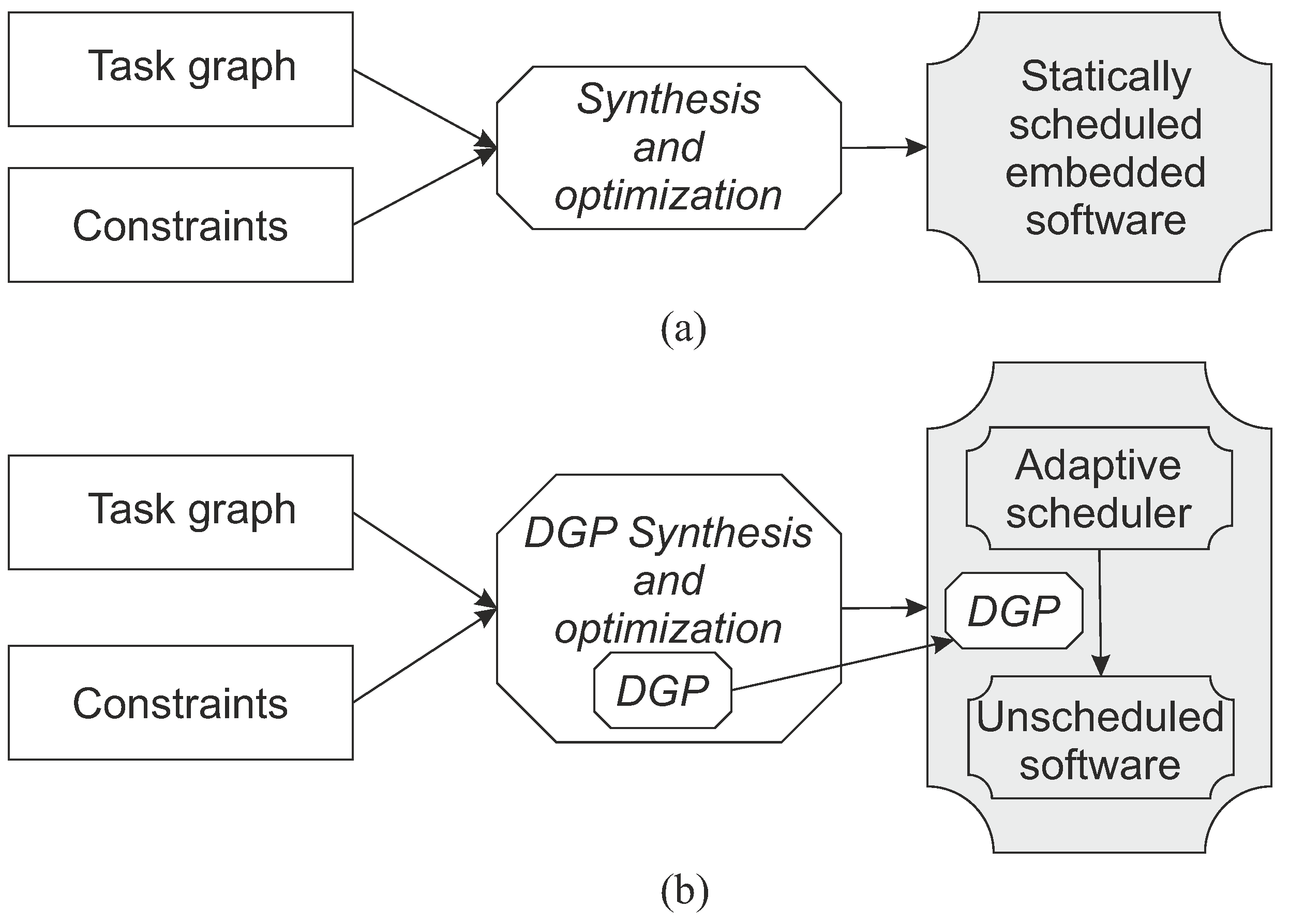
4. Synthesis of Self-Adaptive Scheduler

When DGP is used to optimize task allocation in distributed systems, the genotype represents the optimized scheduling strategy, and the phenotype denotes the final task-implementation schedule. Typically, the phenotype is a description of the target system that corresponds to a static scheduler. This approach incorporates both the phenotype and genotype, utilizing a G2P mapping function within the system. Consequently, a system is developed that features a self-adaptive scheduler.

4.1. System Specification

The behavior of a specialized distributed system is determined by the software running on it. This program is a composition of functions, which could be executed concurrently as separate tasks. The output of some of them can provide input to other tasks, establishing relationships between them. Typically, a directed acyclic graph (DAG), known as a task graph (TG), is used to illustrate the relationships between tasks. In this graph, nodes represent tasks and edges between nodes indicate relationships between tasks. In the context of a multicore system, communication time could be omitted, since the data are presumed to be in shared memory. Figure 3 illustrates an example of a task graph.

4.2. System Hardware

The target system architecture is assumed to be implemented using multi-core ARM processors supporting DynamIQ and DVFS technologies for power management. This configuration includes at least two processing element (PE) categories: energy-efficient PE (e.g., Cortex-A55, Cortex-X2) and high-performance PE (e.g., Cortex-A77, Cortex-X3). Every PE (resource) can run each task of the software. The estimated attributes of these resources, such as the minimum, average, and maximum execution durations for each task, are cataloged in a resource library. Similar evaluations are made regarding the energy consumption of each task. These estimates, encompassing both execution time and energy usage, can be derived by obtaining actual measurements during task execution across various cores with different inputs or through established code analysis techniques [31,32].

Table 2. Sample estimations for tasks.

Task	A55						A77
	min		avg		max		min		avg		max
	t	p	t	p	t	p	t	p	t	p	t	p
T1	3	6	4	9	10	17	1	9	4	22	6	41
T2	4	7	8	14	13	24	3	14	7	30	10	37
T3	3	5	7	14	11	21	1	6	4	23	9	34
T4	2	4	5	11	10	18	2	8	5	27	7	31
T5	5	9	13	23	16	27	3	19	8	38	12	51
T6	4	6	7	11	9	16	5	12	7	21	9	29

presents a sample dataset for ARM Cortex-A55/Cortex-A77, based on the TG depicted in Figure 3. The values in the table correspond to the highest core speeds. The columns in Table 2 are included below:

• Task—task identifier;
• t— estimated execution time;
• p—estimated power consumption;
• Min—shortest case;
• Avg—average case;
• Max—longest case.

Although this example is primarily for illustrative purposes and the values are selected at random, the correlation patterns among these values are comparable (with slight random variances) to those seen in actual benchmark analyses.

4.3. Rating a Quality

The next key point of the proposed approach relies on determining the most efficient schedule building rules that satisfy the conditions listed below:

• The sum of average execution times does not exceed the deadline;
• The frequency of the selected core is not changed during a task execution;
• During the scheduling, the core frequency can be freely selected for each task from the available options;
• The level of an energy consumption is as low as possible;
• The level of self-adaptation is maximized.

The execution time and energy consumption of any solution can easily be determined. However, evaluating self-adaptation requires an appropriate metric. Initially, the system is optimized on the assumption that all tasks will run according to their average times. There could be two cases during the run-time that require rescheduling:

• The recently completed task exceeded its usual duration, which resulted in a violation of the time constraints for the next task.
• The most recently completed task was completed in a shorter time, which provides an opportunity to save energy by reallocating some tasks to low-power cores or reducing the frequency of occupied cores.

To compare both cases, two separate self-adaptivity metrics were defined: $S_{RT}$ and $S_{EC}$.

For the first metric, it is assumed that the makespan of the task graph is fixed. Let $s_i$ represent a scenario that describes when, where, and how long each task is executed, and let $V_s$ represent the set of all scenarios; thus, $V_s$ = $\left\{s_i\right\}$. The self-adaptivity of scenario $s_i$ is defined as follows:

$$sa\left(s_i\right)=\left\{\begin{array}{cc}0\hfill & \mathrm{if}T\left(s_i\right)>D\hfill \\ 1\hfill & \mathrm{if}T\left(s_i\right)\le D\hfill \end{array}\right.$$

(1)

where

$T\left(s_i\right)$—the length of the makespan in scenario $s_i$;

D—a deadline.

The self-adaptivity of the real-time scheduling ($S_{RT}$) is defined by Equation (2).

$$S_{RT}={\displaystyle \frac{{\sum }_{k=1}^{\left|V_s\right|}sa\left(S_k\right)}{\left|V_s\right|}}$$

(2)

The second metrics analyses cases are when the execution time of a task or a group of tasks is shorter than expected. If this situation is described by scenario $r_i$ and a set of all considered scenarios is $V_r=\left\{r_i\right\}$, the $s{a}_{EC}$ metric is defined as Equation (3).

$$sa\left(r_i\right)=\left\{\begin{array}{cc}0\hfill & \mathrm{if}ec\left(r_i\right))>e_s\hfill \\ 1-{\displaystyle \frac{ec\left(r_i\right)-e_{min}}{e_s-e_{min}}}\hfill & \mathrm{if}ec\left(r_i\right)\le e_s\hfill \\ 1\hfill & \mathrm{if}{e}_s=e_{min}\hfill \end{array}\right.$$

(3)

In this context, $e_s$ is the energy used for the initial makespan, $ec\left(r_i\right)$ is the energy consumed by the makespan in scenario $r_i$, and $e_{min}$ denotes the minimum possible energy consumption for the initial makespan (assuming that each task consumes the least amount of energy, without care of time constrains). Thus, the self-adaptive energy consumption ($S_{EC}$) for the makespan is defined as follows:

$$S_{EC}={\displaystyle \frac{{\sum }_{k=1}^{\left|V_r\right|}sa\left(r_k\right)}{\left|V_r\right|}}$$

(4)

Given that the system is optimised for power efficiency, this parameter is defined as

$$P_E={\displaystyle \frac{e_{max}-e_s}{e_{max}}}$$

(5)

where $e_{max}$ is the maximal energy consumption.

Finally, the quality of the given solution is defined as follows:

$$Q=\alpha \ast S_{RT}+\beta \ast S_{EC}+(1-\alpha -\beta )\ast P_E$$

(6)

where

• $\alpha$ and $\beta$ are self-adaptivity coefficients, both ranging between 0.0 and 1.0;
• sum $\alpha +\beta$ does not exceed 1.
• Equation (6) is an example of a multi-objective linear optimization challenge, widely recognized as the predominant technique to address the practical optimization problems of multiple criteria [33].

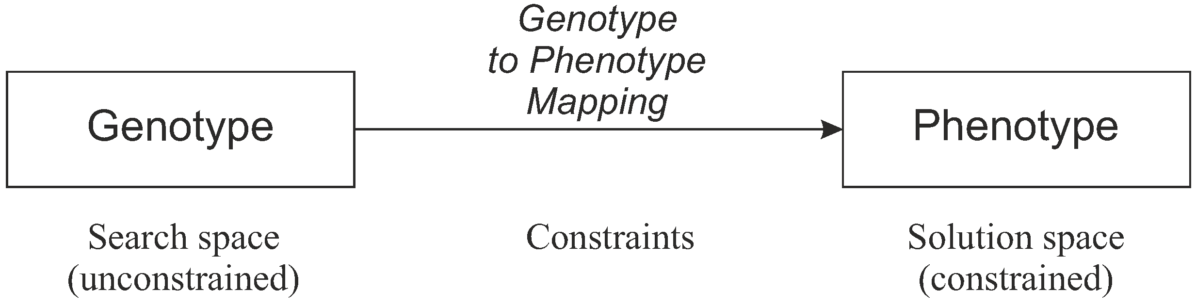
4.4. Genotype and Phenotype

Each member of the population is described by its genotype, and its corresponding phenotype represents the solution (example in Figure 4). The genotype has the shape of a binary tree (example in Figure 4a) that contains a specific method of tasks allocation and scheduling in the target system. Based on it, the final makespan (the phenotype) is generated.

The internal nodes of the TG divide the system into subsystems, while the leaves represent scheduling strategies. Each internal contains information about a cut position (CutPos) that divides the list of tasks into two sublists. The left and right sublists are assigned to the left and right children of the node. A randomly ordered list of all tasks is assigned to the root node. CutPos is also randomly selected during the initial population generation and can be modified if the associated gene is mutated. In Figure 4a, it is assumed that gene G0 divides the system into two subsystems: one with tasks T1, T3, T4, and T6 and the other with tasks T2 and T5.

The strategies of assigning tasks to nodes and placing them in the schedule are as follows:

• The highest performance core;
• The core that consumes the least energy during execution;
• The best ratio of time to energy consumption;
• The core that could start task execution first;
• Considering a start time, the core that finishes task execution first;
• The first available core from these ones that consumes the least energy during execution;
• The fixed assignment defined by the second chromosome.

In Figure 4, how gene G0 divides a list of tasks into two parts is presented. The first part is connected with gene G1, which favors allocating tasks T1, T3, T4, and T6 to the core with minimal energy usage. The rest of the list is connected with gene G2 instructing a scheduler to choose the core that is able to finish tasks T2 and T5 in the shortest time.

In some cases, strict applying strategies could violate time constraints. Thus, they are used with flexibility. If allocating a core according to the preferred strategy is unsuccessful (e.g., the time limit might be missed), the subsequent core or a core with different clock frequency is attempted employing the same approach. This process continues until a viable schedule is obtained or all cores and their frequency options are evaluated (i.e., none of the solutions fulfill the time requirements). To illustrate it more precisely, if the strategy is to use “the most energy efficient core” and the lowest energy-consuming core does not meet the deadline, the scheduler will attempt to increase the clock frequency or use the next core, which could consume more energy but comply with the time limits. In the experiments, typically, the next most energy-efficient core was chosen in such situations, but occasionally, a high-performance core was needed to meet time constraints. This selection process can also occur during run-time when rescheduling is necessary.

The scheduling algorithm is detailed in Algorithm 1. The StaticSchedule() function is executed once to create the system’s initial schedule. Initially, the genotype tree is traversed to find the assignment strategy for each task. Next, for each task, deadlines are calculated. In the next step, tasks are sorted, starting from the task with the shortest deadline. The task with the longest deadline is put at the end of the list. Finally, static scheduling based on the average execution time is conducted. It is similar to the list scheduling method with static priorities. The Reschedule() function is used to formulate the initial schedule and for subsequent rescheduling. When the execution of each task is finished, the actual execution time is compared with the expected time. If there is a difference, whether the task was completed faster or slower than in the initial schedule, a reschedule is performed for all tasks that have not yet started. The following functions are defined: Idle(Rj) returns the nearest time when the resource Rj will be available, Start(Ti) returns the earliest time when the task Ti can be lauched, i.e., when all predecessor tasks have been completed, and execution_time(Ti,Rj) calculates the mean time taken to execute the task Ti utilizing resource Rj.

4.5. Evolution

DGP is an evoloutionary-based algorithm; thus, optimization is achieved by increasing the quality of individuals in each generation. At the start, a random individuals presenting solutions are generated. Successive generations of solutions are generated using genetic operators such as crossover, mutation, and reproduction. In the presented method, genotypes are trees; thus, during crossover in each tree, one branch is chosen randomly. Then, subtrees connected to these branches are swapped. Mutation involves changing the type (which aligns with the scheduling approach) of a node chosen at random within the tree to a different type. Selection and reproduction are performed using a tournament method [34]. More details about the genetic operators used in the described method can be found in [35]. Evolution continues as long as the best solution improves in successive populations. The quality metric Q (6) is used to evaluate fitness.

5. Experimental Results

This chapter starts with a quick introduction before providing the results of previous work, starting from [5] to [4] and then presenting new research.

5.1. Overview of Previous Research

In this study, my methodology was validated using a practical example: a multimedia system (MMS) [36]. Figure 5 shows the MMS task graph. A table presenting the runtime and energy consumption for all tasks was published in [4]. The data reflect performance at the core’s highest speed. These values were derived from measurements taken on the Odroid-XU4 (https://wiki.odroid.com/odroid-xu4/odroid-xu4 [Access: 14 December 2024]) platform. Although this platform relies on the Samsung Exynos5422 CPU (4 × Cortex-A15 + 4 × Cortex-A7 cores), it was chosen due to other developmental platforms being unavailable. Energy consumption was recorded for each task on each core using the Odroid SmartPower 1st generation (Monitoring: Voltage, Current, Watt, Watt-Hour (Sample rate: 10 Hz)). The data were then scaled to A55/A77 cores. Each task’s minimum, typical, and maximum execution times are documented. These execution times were measured by running the programs on each core with three different types of input data. The first type corresponded to the simplest cases with the shortest execution times. The second type represented the most challenging cases with the longest execution times. The third type included the most commonly anticipated input data, referred to as “typical”. Energy consumption is based on the typical execution time.

The impact of self-adaptivity was shown in [4] in Table 3. There is a analysis of how the metrics of self-adaptivity influence a generated solution. When comparing results generated with and without considering the metrics, it could be noticed that the initial solution generated with them is slightly worse than that generated without them. But after any disruption occurs, solutions that are built with an emphasis on self-adaptivity are able to consume less energy. For more examples and detailed explanations, refer to previous work [4].

The decision on using DGP in this kind of problem was made in [29]. A comparison between DGP and the least laxity first algorithm (LLF) was there presented. The main conclusion was that in spite of height efficiency, LLF creates a worse result than DGP.

5.2. Influence of Self-Adaptation on Energy Consumption

Beginning with the research presented in [4], this study explores the influence of self-adaptivity on the energy consumption of systems using not only the big.LITTLE architecture, but also dynamic voltage and frequency scaling (DVFS). The first step was the analysis of the influence of the parameters $\alpha$ and $\beta$ in the fitness function. They control the importance of these factors, with the results presented in

Table 3. Energy cost of the media player system [mJ]. The best results are in italic.

$\alpha$
1.0	1715.00
0.8	1552.00	1578.00
0.6	1550.00	1565.00	1556.00
0.4	1529.00	1517.00	1549.00	1566.00
0.2	1527.00	1532.00	1554.00	1557.00	1570.00
0	1532.00	1534.00	1560.00	1566.00	1534.00	1566.00
	0	0.2	0.4	0.6	0.8	1.0	$\beta$
	The best individuals
$\alpha$
1.0	1713.16
0.8	1571.93	1592.60
0.6	1572.91	1585.76	1564.83
0.4	1559.89	1541.70	1572.34	1577.15
0.2	1544.66	1557.80	1567.73	1571.50	1615.88
0	1555.25	1558.48	1580.86	1585.56	1562.16	1577.58
	0	0.2	0.4	0.6	0.8	1.0	$\beta$
	Average of the population

.

Table 4. Implementationcost in the most optimistic case for the multimedia player system.

$\alpha$
1.0	1705.000
0.8	968.000	972.000
0.6	1011.000	1000.000	980.000
0.4	975.000	981.000	975.000	996.000
0.2	967.000	978.000	1005.000	990.000	1022.000
0	983.000	977.000	1015.000	1002.000	988.000	975.000
	0	0.2	0.4	0.6	0.8	1.0	$\beta$
	The best individuals
$\alpha$
1.0	1890.117
0.8	968.06	971.961
0.6	1011.000	1000.000	980.000
0.4	971.039	981.000	983.164	996.000
0.2	969.922	978.000	970.000	990.000	1021.844
0	983.063	977.016	1015.000	1002.000	988.000	975.000
	0	0.2	0.4	0.6	0.8	1.0	$\beta$
	Average of the population

and

Table 5. Implementationcost in the most pessimistic case for the media player system.

$\alpha$
1.0	1803.00
0.8	1557.00	1584.00
0.6	1554.00	1592.00	1577.00
0.4	1556.00	1532.00	1579.00	1579.00
0.	1539.00	1615.00	1574,00	1573.00	1591.00
0	1541.00	1539.00	1591.00	1566.00	1613.00	1577.00
	0	0.2	0.4	0.6	0.8	1.0	$\beta$
	The best individuals
$\alpha$
1.0	1808.70
0.8	1557.00	1584.00
0.6	1554.00	1592.00	1577.00
0.4	1555.39	1532.00	1579.00	1579.00
0.2	1539.00	1615.00	1583,00	1573.00	1591.00
0	1541.00	1539.02	1591.00	1571.72	1613.00	1577.00
	0	0.2	0.4	0.6	0.8	1.0	$\beta$
	Average of the population

provide additional information by showing energy consumption under scenarios of minimum and maximum task completion times, respectively.

Several key observations were made from the analysis:

• Self-Adaptive Behavior and Energy Usage:
  Self-adaptive behavior was observed to lead to the highest energy consumption. This result is attributed to the system’s tendency to rely predominantly on the fastest resources available, which, while reducing task completion time, increases overall energy demand. The system’s prioritization of adaptability likely causes a shift towards higher-performance (and, thus, higher-energy) cores to maintain flexibility and responsiveness to changing workloads.
• Self-Optimization and Energy Efficiency:
  In contrast, self-optimization was found to facilitate a reduction in energy consumption. However, this approach does not inherently consider the potential benefits of rescheduling tasks across different resources. As a result, while self-optimization effectively reduces energy usage by optimizing resource allocation, it can miss opportunities to further minimize energy consumption by dynamically adjusting task scheduling.
• Energy-Only Evaluation and Resource Utilization:
  When the evaluation metric focused only on energy consumption, it was expected to produce the most energy efficient solution for the initial task scheduling. However, this approach exhibited a significant drawback. By greedily selecting the lowest-energy resources early in the scheduling process, the system was compelled to rely on more powerful and energy-consuming resources, especially at the end of the schedule. This behavior resulted in an overall increase in energy consumption, contrary to the intended goal of minimizing it.
• Balanced Multi-Criteria Evaluation:
  The most effective results were achieved when the evaluation uses all three criteria: self-adaptation, self-optimization, and energy consumption. This comprehensive approach allowed the algorithm to avoid local minima by considering the trade-offs between adaptability, optimization, and energy efficiency. In effect, the system was able to achieve a more balanced allocation of tasks across resources, leading to improved energy efficiency without sacrificing performance.

These results suggest that while individual focus on self-adaptation, self-optimization, or energy consumption can lead to suboptimal outcomes, a balanced approach that integrates all three aspects is crucial for optimizing both energy efficiency and system performance.

5.3. Implementing DVFS in the Presented Method

One of the primary challenges encountered during the implementation of the discussed extension to the existing method was defining the relationship between different operating frequencies of a processing core. Specifically, it was essential to determine that a change in frequency represents a different state of an existing resource rather than a completely distinct resource. This challenge was solved by an idea that each frequency state is a quasi-independent resource. However, the utilization of any specific state excludes the possibility of deploying the remaining states for other tasks. This approach ensures that the same physical core cannot be used simultaneously at different frequencies for different tasks.

To establish the relationship between execution time and energy consumption relative to the data presented in [4], the characteristics of time frequency and energy frequency described in [37] were used. This method provided a foundation for estimating the parameters needed to convert the required time and energy from a given frequency based on the maximum operating frequency of the Samsung Exynos 980 processor. The conversion factors specific to the A55 core are detailed in

Table 6. Influence of changing frequency into speed and energy consumption on A55 core.

Frequency [GHz]	In Relation to the Highest Frequency
	Time	Energy Consumption
0.2	918.29%	2.87%
0.3	681.34%	6.17%
0.4	512.71%	9.71%
0.5	392.69%	13.53%
0.6	307.28%	17.64%
0.7	246.49%	22.06%
0.8	203.23%	26.83%
0.9	172.44%	31.96%
1.0	150.53%	37.49%
1.1	134.94%	43.44%
1.2	123.84%	49.84%
1.3	115.94%	56.74%
1.4	110.32%	64.17%
1.5	106.32%	72.17%
1.6	103.47%	80.78%
1.7	101.44%	90.05%
1.8	100.00%	100.00%

, while those for the A77 core are presented in

Table 7. Influence of changing frequency into speed and energy consumption on A77 core.

Frequency [GHz]	In Relation to the Highest Frequency
	Time	Energy Consumption
0.2	1341.30%	3.78%
0.3	1018.50%	5.24%
0.4	779.44%	6.87%
0.5	602.40%	8.69%
0.6	471.28%	10.71%
0.7	374.17%	12.97%
0.8	302.25%	15.48%
0.9	248.99%	18.28%
1.0	209.55%	21.40%
1.1	180.34%	24.88%
1.2	158.70%	28.76%
1.3	142.68%	33.08%
1.4	130.81%	37.90%
1.5	122.02%	43.26%
1.6	115.52%	49.24%
1.7	110.70%	55.91%
1.8	107.13%	63.33%
1.9	104.48%	71.61%
2.0	102.52%	80.83%
2.1	101.07%	91.11%
2.2	100.00%	100.00%

.

5.4. Effects of Introduced Improvements

The results of the experiment are summarized in Table 8. For comparison purposes, Table 8 also contains schedules based on single-strategy approaches, each of which was described in Section 4.4. These new experiments allow for a direct comparison of the effectiveness of different strategies and to check if any one approach is significantly better than the others.

In Figure 6, Figure 7, Figure 8, Figure 9 and Figure 10, the schedules generated for the most expected completion times are illustrated:

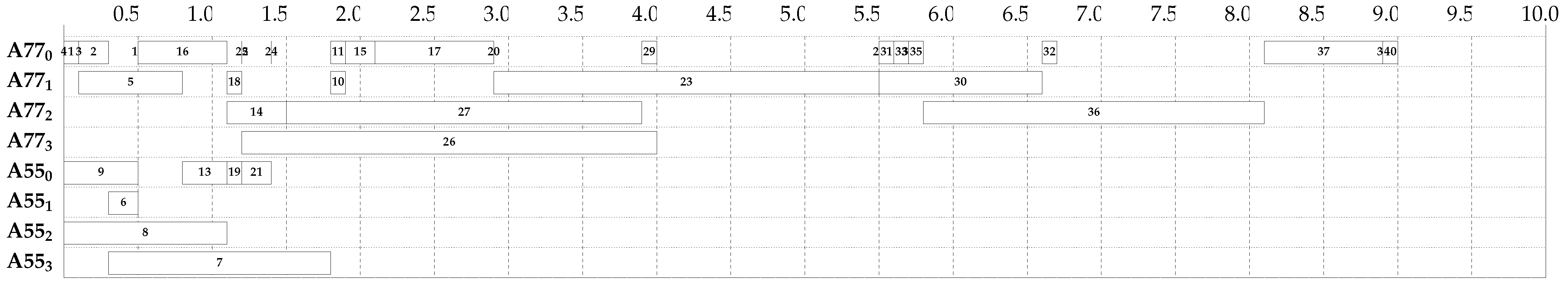
• Figure 6 presents a schedule that does not consider time buffers or DVFS (dynamic voltage and frequency scaling). The behavior of the system here indicates an attempt to save energy, but this decreases flexibility and responsiveness to potential delays.
• Figure 7 displays a schedule that incorporates time buffers but not DVFS. This approach increases the time resistance of the system for time delays, but the initial scheduling consumes a little more energy, because there is a little more pressure to choose more performance-oriented cores.
• Figure 8, Figure 9 and Figure 10 present schedules generated during evolutionary processes. The differences between these schedules are minimal, primarily focused on the duration of certain tasks. These variations are different in buffer lengths and the frequencies of the used cores.

The analysis reveals several key insights into the performance of different strategies:

• Speed-Oriented Strategies: Approaches focused basically on speed often yield suboptimal results, as they do not leverage energy-saving opportunities. In some optimistic scenarios, these strategies can even lead to worse results, as they may over-utilize high-performance resources, leading to unnecessary energy consumption.
• Energy-Efficient Strategies: While energy-efficient strategies are effective in saving energy under optimistic conditions, they tend to result in higher initial energy usage. This is due to time constraints necessitating the use of more powerful, energy-intensive resources early in the scheduling process to meet deadlines.
• Multi-Criteria Evaluation: The best results were achieved using a multi-criteria fitness function, which balanced speed and energy efficiency. The optimal result was achieved when the parameters of the fitness function were set to $\alpha =40\%$ and $\beta =20\%$. This configuration favored the creation of time buffers that encouraged a more diversified use of resources, leading to a more balanced and efficient schedule. The schedule generated under these conditions is illustrated in Figure 10.

Table 8. Experimental results (energy cost [mJ]). In addition to the individuals generated during evolution, control individuals representing the use of only one type of strategy were added.

Individuals	Optimistic Case	The Most Expected Case	Pessimistic Case
Only the fastest	2053	1890	1880
Only the most energy efficient	477	1699	1688
Only the best ratio of time to energy consumption	468	1570	1556
Only determined by the alternative gene	1661	1736	1696
Only the fastest available core	1903	1780	1880
Only the fastest finishing core	1868	1725	2047
Only the most energy-efficient core that is available first	1903	1780	1880
The best one achieved when $\alpha =0\%$ and $\beta =0\%$ (Figure 8)	565	1501	1516
The best one achieved when $\alpha =40\%$ and $\beta =20\%$ Figure 9)	562	1484	1503
The best one achieved when $\alpha =20\%$ and $\beta =20\%$ (Figure 10)	572	1562	1590
The best one achieved when $\alpha =20\%$ and $\beta =20\%$ without DVFS	981	1517	1532

Table 8. Experimental results (energy cost [mJ]). In addition to the individuals generated during evolution, control individuals representing the use of only one type of strategy were added.

Individuals	Optimistic Case	The Most Expected Case	Pessimistic Case
Only the fastest	2053	1890	1880
Only the most energy efficient	477	1699	1688
Only the best ratio of time to energy consumption	468	1570	1556
Only determined by the alternative gene	1661	1736	1696
Only the fastest available core	1903	1780	1880
Only the fastest finishing core	1868	1725	2047
Only the most energy-efficient core that is available first	1903	1780	1880
The best one achieved when $\alpha =0\%$ and $\beta =0\%$ (Figure 8)	565	1501	1516
The best one achieved when $\alpha =40\%$ and $\beta =20\%$ Figure 9)	562	1484	1503
The best one achieved when $\alpha =20\%$ and $\beta =20\%$ (Figure 10)	572	1562	1590
The best one achieved when $\alpha =20\%$ and $\beta =20\%$ without DVFS	981	1517	1532

Figure 6. Task scheduling without taking into account time buffers and without DVFS (time in [ms]).

Figure 6. Task scheduling without taking into account time buffers and without DVFS (time in [ms]).

Figure 7. Task scheduling with time buffers and without DVFS (time in [ms]).

Figure 7. Task scheduling with time buffers and without DVFS (time in [ms]).

Figure 8. Best individual when $\alpha =0\%$, $\beta =0\%$ and DVFS is taken into account (time in [ms]).

Figure 8. Best individual when $\alpha =0\%$, $\beta =0\%$ and DVFS is taken into account (time in [ms]).

Figure 9. Best individual when $\alpha =40\%$, $\beta =20\%$ and DVFS is taken into account (time in [ms]).

Figure 9. Best individual when $\alpha =40\%$, $\beta =20\%$ and DVFS is taken into account (time in [ms]).

Figure 10. Best individual when $\alpha =20\%$, $\beta =20\%$ and DVFS is taken into account (time in [ms]).

Figure 10. Best individual when $\alpha =20\%$, $\beta =20\%$ and DVFS is taken into account (time in [ms]).

Compared to the schedules shown in Figure 6 and Figure 7, this approach shifted some tasks from energy-efficient to high-performance cores, but at reduced operating frequencies. This adjustment proved to be a more effective solution, as it maintained a balance between energy savings and performance requirements. The resulting schedule demonstrates the benefits of a multi-criteria approach to task scheduling, optimizing both energy consumption and task completion time.

Figure 10 was added to highlight the influence of self-adaptive and self-optimization on the final solution. The parameters $\alpha$ and $\beta$ are close to the optimal values in Figure 9. Despite that only the $\alpha$ factor was slightly described, the results are significantly worse.

6. Conclusions

In this paper, a novel extension of the automatic generation of a self-adaptive scheduler was presented. It was assumed that the software will run on a platform where the big.LITTLE architecture and DVFS technology are used. The use of a multi-criteria evaluation function consistently yielded the most effective scheduling examples. Moreover, an extension to the original method was proposed, allowing the cores to operate not only at full frequency but also at lower frequencies. This modification was designed to reduce energy consumption while ensuring that the system could still effectively manage possible timing delays.

The proposed extension demonstrated a significant improvement in energy efficiency, as evidenced by the comparisons in Table 3, Table 4 and Table 5 and Table 8. In particular, the solution provided substantial gains in scenarios that involve faster task completion times. This improvement is very important for battery-powered devices, such as those commonly used in the Internet of Things (IoT), where energy efficiency is a critical aspect.

The results demonstrate that the improved method offers an effective solution to balancing performance and energy usage, especially in scenarios where the time to perform the task is shorter than expected. However, this method could still be developed. Future research could investigate the incorporation of novel scheduling strategies, the real-time adjustment of resource frequencies during task execution, and the improvement of the mapping function to increase overall system performance.

References

1. Yen, T.Y.; Wolf, W. Hardware-Software Co-Synthesis of Distributed Embedded Systems; Springer: Boston, MA, USA, 1996. [Google Scholar] [CrossRef]
2. Humrick, M. Exploring DynamIQ and ARM’s New CPUs: Cortex-A75, Cortex-A55. 2017. Available online: https://www.anandtech.com/show/11441/dynamiq-and-arms-new-cpus-cortex-a75-a55 (accessed on 31 October 2023).
3. Macías-Escrivá, F.D.; Haber, R.; del Toro, R.; Hernandez, V. Self-adaptive systems: A survey of current approaches, research challenges and applications. Expert Syst. Appl. 2013, 40, 7267–7279. [Google Scholar] [CrossRef]
4. Deniziak, S.; Ciopiński, L. Synthesis of self-adaptable energy aware software for heterogeneous multicore embedded systems. Microelectron. Reliab. 2021, 123, 114184. [Google Scholar] [CrossRef]
5. Deniziak, S.; Ciopiński, L. Synthesis of Power Aware Adaptive Embedded Software Using Developmental Genetic Programming. In Recent Advances in Computational Optimization: Results of the Workshop on Computational Optimization WCO 2015; Fidanova, S., Ed.; Springer International Publishing: Cham, Switzerland, 2016; pp. 97–121. [Google Scholar] [CrossRef]
6. Salehie, M.; Tahvildari, L. Self-Adaptive Software: Landscape and Research Challenges. ACM Trans. Auton. Adapt. Syst. 2009, 4, 1–42. [Google Scholar] [CrossRef]
7. Schmeck, H.; Müller-Schloer, C.; Çakar, E.; Mnif, M.; Richter, U. Adaptivity and Self-Organization in Organic Computing Systems. ACM Trans. Auton. Adapt. Syst. 2010, 5, 1–32. [Google Scholar] [CrossRef]
8. Yeom, K.; Park, J.H. Morphological approach for autonomous and adaptive systems based on self-reconfigurable modular agents. Future Gener. Comput. Syst. 2012, 28, 533–543. [Google Scholar] [CrossRef]
9. Vogel, T.; Neumann, S.; Hildebrandt, S.; Giese, H.; Becker, B. Model-Driven Architectural Monitoring and Adaptation for Autonomic Systems. In Proceedings of the 6th International Conference on Autonomic Computing, Barcelona, Spain, 15–19 June 2009; Association for Computing Machinery: New York, NY, USA, 2009. ICAC ’09. pp. 67–68. [Google Scholar] [CrossRef]
10. Leitao, P. Holonic Rationale and Bio-inspiration on Design of Complex Emergent and Evolvable Systems. In Transactions on Large-Scale Data- and Knowledge-Centered Systems I; Hameurlain, A., Küng, J., Wagner, R., Eds.; Springer: Berlin/Heidelberg, Germany, 2009; pp. 243–266. [Google Scholar] [CrossRef]
11. Chen, T. A self-adaptive agent-based fuzzy-neural scheduling system for a wafer fabrication factory. Expert Syst. Appl. 2011, 38, 7158–7168. [Google Scholar] [CrossRef]
12. Oreizy, P.; Gorlick, M.M.; Taylor, R.N.; Heimhigner, D.; Johnson, G.; Medvidovic, N.; Quilici, A.; Rosenblum, D.S.; Wolf, A.L. An architecture-based approach to self-adaptive software. IEEE Intell. Syst. Their Appl. 1999, 14, 54–62. [Google Scholar] [CrossRef]
13. Higuera-Toledano, M.T.; Brinkschulte, U.; Rettberg, A. (Eds.) Self-Organization in Embedded Real-Time Systems; Springer Science+Business Media: New York, NY, USA, 2012. [Google Scholar] [CrossRef]
14. Pułka, A.; Milik, A. Dynamic Rescheduling of Tasks in Time Predictable Embedded Systems. IFAC Proc. Vol. 2012, 45, 305–310. [Google Scholar] [CrossRef]
15. Gharsellaoui, H.; Ktata, I.; Kharroubi, N.; Khalgui, M. Real-time reconfigurable scheduling of multiprocessor embedded systems using hybrid genetic based approach. In Proceedings of the 2015 IEEE/ACIS 14th International Conference on Computer and Information Science (ICIS), Las Vegas, NV, USA, 28 June–1 July 2015; pp. 605–609. [Google Scholar] [CrossRef]
16. Calhoun, K.M.; Deckro, R.F.; Moore, J.T.; Chrissis, J.W.; Van Hove, J.C. Planning and re-planning in project and production scheduling. Omega 2002, 30, 155–170. [Google Scholar] [CrossRef]
17. Van de Vonder, S.; Demeulemeester, E.; Herroelen, W. A classification of predictive-reactive project scheduling procedures. J. Sched. 2007, 10, 195–207. [Google Scholar] [CrossRef]
18. El Sakkout, H.; Wallace, M. Probe backtrack search for minimal perturbation in dynamic scheduling. Constraints 2000, 5, 359–388. [Google Scholar] [CrossRef]
19. Al-Fawzan, M.; Haouari, M. A bi-objective model for robust resource-constrained project scheduling. Int. J. Prod. Econ. 2005, 96, 175–187. [Google Scholar] [CrossRef]
20. Bambagini, M.; Marinoni, M.; Aydin, H.; Buttazzo, G. Energy-Aware Scheduling for Real-Time Systems: A Survey. ACM Trans. Embed. Comput. Syst. 2016, 15, 1–34. [Google Scholar] [CrossRef]
21. Scordino, C.; Abeni, L.; Lelli, J. Energy-Aware Real-Time Scheduling in the Linux Kernel. In Proceedings of the 33rd Annual ACM Symposium on Applied Computing, Pau, France, 9–13 April 2018; Association for Computing Machinery: New York, NY, USA, 2018. SAC ’18. pp. 601–608. [Google Scholar] [CrossRef]
22. Zeng, G.; Yokoyama, T.; Tomiyama, H.; Takada, H. Practical Energy-Aware Scheduling for Real-Time Multiprocessor Systems. In Proceedings of the 2009 15th IEEE International Conference on Embedded and Real-Time Computing Systems and Applications, Beijing, China, 24–26 August 2009; pp. 383–392. [Google Scholar] [CrossRef]
23. Deniziak, S.; Ciopinski, L. Design for Self-Adaptivity of Real-Time Embedded Systems Using Developmental Genetic Programming. In Proceedings of the 2018 Conference on Electrotechnology: Processes, Models, Control and Computer Science (EPMCCS), Kielce, Poland, 12–14 November 2018; pp. 1–5. [Google Scholar] [CrossRef]
24. Li, X.; Mo, L.; Kritikakou, A.; Sentieys, O. Approximation-Aware Task Deployment on Heterogeneous Multicore Platforms with DVFS. IEEE Trans. Comput.-Aided Des. Integr. Circuits Syst. 2022, 42, 2108–2121. [Google Scholar] [CrossRef]
25. Shukla, S.K.; Pant, B.; Viriyasitavat, W.; Verma, D.; Kautish, S.; Dhiman, G.; Kaur, A.; Srihari, K.; Mohanty, S.N. An integration of autonomic computing with multicore systems for performance optimization in Industrial Internet of Things. IET Commun. 2022. [Google Scholar] [CrossRef]
26. Deniziak, S.; Płaza, M.; Arcab, L. Approach for Designing Real-Time IoT Systems. Electronics 2022, 11, 4120. [Google Scholar] [CrossRef]
27. Koza, J.; Poli, R. Genetic Programming. In Search Methodologies; Burke, E., Kendall, G., Eds.; Springer: Boston, MA, USA, 2005; pp. 127–164. [Google Scholar] [CrossRef]
28. Koza, J.R.; Bennett, F.H., III; Andre, D.; Keane, M.A. Evolutionary design of analog electrical circuits using genetic programming. In Proceedings of the Adaptive Computing in Design and Manufacture; Springer: London, UK, 1998; pp. 177–192. [Google Scholar] [CrossRef]
29. Deniziak, S.; Ciopiński, L. Synthesis of power aware adaptive schedulers for embedded systems using developmental genetic programming. In Proceedings of the Federated Conference on Computer Science and Information Systems (FedCSIS), Lodz, Poland, 13–16 September 2015; IEEE: Piscataway, NJ, USA, 2015; pp. 449–459. [Google Scholar] [CrossRef]
30. Wang, Y.; Liu, H.; Liu, D.; Qin, Z.; Shao, Z.; Sha, E.H.M. Overhead-aware energy optimization for real-time streaming applications on multiprocessor System-on-Chip. ACM Trans. Des. Autom. Electron. Syst. 2011, 16, 1–32. [Google Scholar] [CrossRef]
31. Fornaciari, W.; Gubian, P.; Sciuto, D.; Silvano, C. Power estimation of embedded systems: A hardware/software codesign approach. IEEE Trans. Very Large Scale Integr. (VLSI) Syst. 1998, 6, 266–275. [Google Scholar] [CrossRef]
32. Ermedahl, A.; Engblom, J. Execution Time Analysis for Embedded Real-Time Systems. In Handbook of Real-Time and Embedded Systems; Lee, I., Joseph, Y.-T., Leung, S.H.S., Eds.; Chapman & Hall/CRC: New York, NY, USA, 2008; pp. 437–455. [Google Scholar]
33. Noghin, V.D. Linear scalarization in multi-criterion optimization. Sci. Tech. Inf. Process. 2015, 42, 463–469. [Google Scholar] [CrossRef]
34. Michalewicz, Z. Genetic Algorithms+ Data Structures= Evolution Programs; Springer: Berlin/Heidelberg, Germany, 1996. [Google Scholar] [CrossRef]
35. Sapiecha, K.; Ciopiński, L.; Deniziak, S. An application of developmental genetic programming for automatic creation of supervisors of multi-task real-time object-oriented systems. In Proceedings of the 2014 Federated Conference on Computer Science and Information Systems (FedCSIS), Warsaw, Poland, 7–10 September 2014; IEEE: Piscataway, NJ, USA, 2014; pp. 501–509. [Google Scholar] [CrossRef]
36. Hu, J.; Marculescu, R. Energy-and performance-aware mapping for regular NoC architectures. IEEE Trans. Comput.-Aided Des. Integr. Circuits Syst. 2005, 24, 551–562. [Google Scholar] [CrossRef]
37. Ara, G.; Cucinotta, T.; Mascitti, A. Simulating execution time and power consumption of real-time tasks on embedded platforms. In Proceedings of the 37th ACM/SIGAPP Symposium on Applied Computing, Virtual Event, 25–29 April 2022; Association for Computing Machinery: New York, NY, USA, 2022. SAC ’22. pp. 491–500. [Google Scholar] [CrossRef]
Figure 1. Developmental genetic programming.
Electronics 14 00556 g001
Figure 2. Design and optimization approaches: (a) conventional and (b) suggested. Software for an embedded system is highlighted with a greyed background.
Electronics 14 00556 g002
Figure 3. Sample task graph.
Electronics 14 00556 g003
Figure 4. Example of a genotype (a) and, generated from it, a phenotype (b).
Electronics 14 00556 g004
Figure 5. Multimedia system task graph.
Electronics 14 00556 g005