Bidirectional Pattern Recognition and Prediction of Bending-Active Thin Sheets via Artificial Neural Networks

Abstract

Currently, active-bending structures and their shape optimization techniques have become a hot topic in the design of spatial structures and freeform buildings. However, their form-finding process is usually time-consuming, and the application of finite element methods (FEM) requires huge computational effort. In the face of these challenges, artificial intelligence techniques have great potential for application and bring many important advantages to this field. In this paper, we propose a novel, data-driven, bidirectional prediction method based on artificial neural networks. It can both forward infer the bending deformation shapes of a thin plate under specific complex conditions and reverse infer the boundary conditions necessary for a given bending shape. In comparison to traditional active-bending simulation, the proposed method is quicker and simpler to utilize during the design process and facilitates reverse predictions. Communication between design and construction can be facilitated to ensure quality and efficiency in the construction of relevant bent structural components. It is experimentally demonstrated that the network can control the mean value of prediction deviation below 40 mm for a 4 m × 0.5 m aluminum plate.

1. Introduction

Active bending is a structural design concept whose core idea is to use bending as part of the self-forming process [1]. This concept was first proposed by Julian Lienhard et al. [2] in their research in 2013. In recent years, the application prospects of active bending have been extensive in the fields of architecture and engineering, as it can promote the innovative and sustainable development of structural design. For example, it is applied in creating self-forming structures that can automatically adjust their shape according to environmental changes or flexible use requirements [3], and deployable structures such as deployable antennas and collapsible tubes in space applications. Simultaneously, innovation and research in the field of active-bending materials are crucial.

Compared with traditional manufacturing techniques for building components with curved geometries, active bending is regarded as a method of generating curved structural forms and high structural stiffness from simple straight or flat elements through elastic deformation [4,5]. The advantages include the ability to use thin components to achieve very small bending radii; the ability to maintain low bending stresses with an adequate residual load capacity; and the ability to couple multiple bending elements and their bending preloads to achieve the necessary stiffness [6]. In architectural design, active-bending structures can be used to construct buildings or components that can bend according to environmental conditions. One of the most well-known examples of such a structure is the “Plydome”, designed by Buckminster Fuller in 1957 [3] (Figure 1). Furthermore, Mauricio Soto Rubio built the “experimental pavilion” during the 5-day “block week” at the University of Calgary, showcasing the potential of the rapid assembly of active-bending structures and the use of simple methods to explore spatial installations [7] (Figure 2).

On the one hand, active bending can be viewed as an approach rather than a specific structural type when viewed through the lens of construction techniques. Therefore, it is easier to apply to efficient structural design [8,9,10]. This concept emphasizes actively considering the bending performance of materials in the design and construction process to achieve more flexible, intelligent, and innovative structures. In this method, the bending performance of materials is viewed as a resource, not just a limitation. By actively considering the bending performance of materials, one can create more adaptable and flexible structures that can adapt to different environments and needs. Additionally, this method enhances structural efficiency and minimizes material waste [11,12,13]. On the other hand, structural studies have found that the behavior of active structures does not belong to an explicitly predictable category and that their output geometry is the result of a tight interaction between form, forces, material characteristics, and boundary conditions (e.g., the supports, length, cross-section, and material properties of the bent element) [14,15]. Their load bearing depends heavily on the various topological and geometric expressions that may be generated, and dynamic simulations involving highly nonlinear behavior result in a form-finding process, which is often time-consuming. At the same time, the finite element method (FEM), which is widely used in science and engineering for structural analysis, requires a large amount of computation and is often slow, making it impossible to achieve real-time performance in the presence of complex material behavior or detailed models [16]. Currently, there is still a considerable gap and discontinuity between the increasingly precise computational design stage and the often manual/empirical manufacturing and construction stage of curved active structures from design to construction [17]. Therefore, this paper aims to enable fast simulation in active bending and directly drive the interactive optimization of the construction process.

This study combines finite element analysis (FEM) and machine learning (ML) to optimize the solution process of complex problems by utilizing their complementarity to some extent. FEM provides basic theoretical support in engineering and physics, while ML can handle more complex and larger-scale data and provide more practical approximate solutions. This integrated application strategy may provide new methods and possibilities for engineering and scientific research.

In practice, active-bending structures usually have complex nonlinear and anisotropic bending stiffness properties. Due to their complexity, the form-finding process of bending often takes a long time, and inaccuracies are often present in the simulation techniques making the design process of bending-active structures particularly inconvenient for designers. To solve these problems, we propose a bidirectional prediction method using neural networks. Using this method, we predict the boundary conditions and deformation geometry of bending-active thin plates by directly learning the bending characteristics from sample data and studying specific regression-based neural network algorithms to minimize errors. Compared with traditional methods, the method proposed in this study has the following characteristics:

• It helps to overcome the constraints of traditional physical parameter measurement by avoiding the requirement to directly measure complex physical parameters;
• It improves the simulation accuracy of complex structures and provides a more flexible method for structural design and analysis.

2. Related Works

2.1. Research on Active-Bending Simulation and Analysis

2.1.1. Previews Analysis Methods

In the design and study of active-bending structures, behavior simulation and analysis are the most critical and important issues. When exploring this issue, researchers adopt different types of analysis methods: behavior-based approaches, geometry-based approaches, or integrated approaches [2].

Behavior-based approaches mainly focus on the behavior of materials and their elastic deformation ability. By applying external loads and allowing structural deformation, the final shape is obtained from the residual stress remaining after the removal of external loads, as seen in some rural architectures.

Geometry-based approaches mainly focus on the geometric characteristics of the structure and its ability to deform into the desired shape (Figure 3). They create a geometric model of the structure and then apply external loads to deform it into the desired shape. Buckminster Fuller’s layered structure mentioned above is an example. These intricate structures are derived from geometric patterns, which optimize the use of materials and the stability of the structure (Lienhard, 2018) [3].

Integrated approaches integrate the characteristics of the two aforementioned approaches, reconciling intuition with scientific rigor. For example, in 2010, the Institute for Computational Design (ICD) and the Institute of Building Structures and Structural Design (ITKE) designed and constructed a temporary research pavilion (Figure 4). The result was a bending-active structure made entirely of extremely thin, elastically bent plywood strips. A curve-matching algorithm was created to capture the buckling behavior of the thin plate material under compressive force. It formed a central aspect of the information model and was based on data derived from physical form-finding experiments (Figure 5) [18,19].

In addition, the 2015-16 ICD-ITKE research pavilion project (Figure 6) [20] integrated computer design, biomimicry, and manufacturing processes using a dual bottom-up design concept based on natural baffle-structure biomimicry research and the robotic-sewing technology application of thin plywood (Figure 7). The design team developed a manufacturing technology that can elastically bend double-layer plywood from the analysis of the construction form of sand dollars. By introducing fiber-sewing technology into wood construction, lightweight and high-performance wood shell modules become possible.

Overall, these methods have their own advantages and disadvantages. Behavior-based methods emphasize theoretical analysis and experimental validation and can predict structures more accurately, but they may require a large amount of computational and experimental data. Geometry-based methods are relatively intuitive and easy to implement but usually require experience and intuition to guide the design; they may also be limited by the material properties of the structure.

2.1.2. Problems in Existing Analysis Methods of Bending-Active Geometry

Currently, for active-bending structures, accurately predicting the large deformation geometry and structural performance of thin plates is the biggest challenge due to the complexity of thin-plate bending structures and the uncertainties that arise during the bending process. The design and construction of bending-active systems are closely related to structural principles and construction standards. However, it is still challenging to predict the construction process of active bending at the design stage and to reflect design concepts in active-bending construction due to the experimental uncertainty of bending-active structures, the difficulty of the simple replication or generalization of the design process, and the rapidly advancing designs and materials [17]. When solving the large deformation geometry problems of thin plates, scientists have adopted various new techniques, including numerical simulation, physical experiments, and other methods, to better understand and analyze the deformation behavior of thin plates. Generally, their simulation and prediction techniques can be divided into two main categories: one that focuses on real-time physical simulation, and another that focuses on accurate structural behavior through finite element analysis [5].

Real-time-based methods, such as the Rhinoceros ® plugin Kangaroo Physics, focus on fast feedback on possible curved geometries. Their core lies in using a Dynamic Relaxation solver (DR) [22] to calculate mesh deformation, which requires the introduction of the total mass value and damping coefficient into the calculation model [23,24]. During the simulation process, the system converges to the equilibrium position representing the final curved geometry.

For instance, Kangaroo implements a time integration of Newton’s second law using a semi-implicit Euler method [25]. At every iteration with time step $\mathrm{\Delta }t$ after time t, the solver computes the nodal velocities $v_i^{t+\mathrm{\Delta }t}$ using the nodal forces $F_i^t$ from the previous update and masses $M_i$ and then obtains the positions $x_i^{t+\mathrm{\Delta }t}$ using the new velocities:

$$\left\{\begin{array}{cc}\hfill v_i^{t+\mathrm{\Delta }t}=& v_i^t+\mathrm{\Delta }t{\displaystyle \frac{F_i^t}{M_i}}\hfill \\ \hfill x_i^{t+\mathrm{\Delta }t}=& x_i^t+\mathrm{\Delta }t{v}_i^{t+\mathrm{\Delta }t}\hfill \end{array}\right.$$

(1)

This is a conditionally stable integration scheme with a wide stability region, meaning that it has very good energy conservation [26].

However, there are some challenges with this approach. In simulation calculations, setting parameters, such as the point mass, damping coefficient, spring hardness, etc., is crucial. These parameters usually have strong randomness, making it difficult to accurately reflect the actual and physical properties of the material. This unpredictability may result in simulation accuracy falling short of specifications, particularly when dealing with intricate surface forms and material characteristics [27].

The finite element method is a general numerical method for solving partial differential equations. It is now acknowledged as a standard in the field of structural analysis and is often used to solve various engineering problems [28]. This method converts a continuous physical problem into several discrete elements by dividing the entire solution domain (such as a structure or fluid domain) into many small geometric units, called finite elements, and numerically approximates them to obtain an approximate solution to the overall problem [29]. Programs like SOFiSTiK and Abaqus 2022 have made it possible for designers to forecast complex equilibrium states and compute stresses and deformations in structures undergoing significant deformations in recent years. As an example of finite element analysis software, Abaqus 2022 employs the central difference method for explicit time integration of equations of motion, using the dynamics of one incremental step to calculate the dynamics of the next incremental step, which is typically set in the range from 10,000 to 1,000,000 incremental steps for a standard simulation. The method’s general steps are described below.

First, the kinetic equilibrium equations are established. At the beginning of each incremental step, Abaqus 2022 solves the dynamical equilibrium equation (Equation (2)) based on the node mass matrix M and the external force P, as well as the internal force I of the cell, to obtain the node acceleration u:

$$\begin{array}{c}\hfill Mu=P-I\end{array}$$

(2)

Then, at time point t, the node acceleration is calculated based on the current dynamic conditions:

$$\begin{array}{c}\hfill {\left.u\right|}_{\left(t\right)}={\left.M^{-1}·(P-I)\right|}_{\left(t\right)}\end{array}$$

(3)

Next, the acceleration is integrated over time using the central difference method to obtain the change in velocity, and then the velocity is updated accordingly. Subsequently, the change in velocity is added to the velocity at the midpoint of the previous incremental step to obtain the velocity at the midpoint of the current incremental step. Finally, the displacement at the end of the incremental step is obtained by integrating the velocity over time:

$${\left.u\right|}_{\left(t+\frac{\mathrm{\Delta }t}{2}\right)}={\left.u\right|}_{\left(t-\frac{\mathrm{\Delta }t}{2}\right)}+{\left.{\displaystyle \frac{{\left.\mathrm{\Delta }t\right|}_{(t+\mathrm{\Delta }t)}+{\left.\mathrm{\Delta }t\right|}_{\left(t\right)}}{2}}u\right|}_{\left(t\right)}$$

(4)

The state at the end of an incremental step depends only on the displacement, velocity, and acceleration at the beginning of that incremental step. This method is capable of accurately integrating a constant acceleration but requires that the time increment be small enough to ensure that the acceleration is approximately constant within the incremental step. The strain increment of the cell is then calculated from the strain rate, and then the material’s intrinsic relationship is used to calculate the stress $\sigma$:

$$\begin{array}{c}\hfill \sigma (t+\mathrm{\Delta }t)=f\left({\sigma }_{\left(t\right)},d\epsilon \right)\end{array}$$

(5)

The calculated stresses are related to the geometrical properties of the units and integrated to obtain the internal forces at the nodes $I_{t+\mathrm{\Delta }t}$. The time is then updated to $t+\mathrm{\Delta }t$, where $\mathrm{\Delta }t$ is the time increment for that incremental step. The cycle of calculations then returns to the kinetic equilibrium equations and continues for the next incremental step. By following the steps listed above, Abaqus 2022 is capable of solving dynamic problems that require small time steps for correct simulation. Therefore, it is a perfect fit for analyzing complex engineering problems involving large deformations and high velocities.

Compared with other numerical methods, the finite element method provides the most complete and accurate mechanical description and is an important tool for correctly evaluating the mechanical behavior and structural capabilities of flexural active structures [30]. Compared to real-time physical simulation, finite element simulation provides a more intuitive way to demonstrate the evolution of internal stresses in materials with deformation processes. Complex nonlinearities and large deformations can be considered, helping engineers evaluate the performance of structures and optimize designs and making engineering designs more accurate and reliable. It provides the most complete and accurate mechanical description, making it an important tool for correctly evaluating the mechanical behavior and structural capabilities of bending-active structures [5].

However, the finite element method still has some limitations. For example, in explicit dynamic analyses, a large number of small time steps are often required to ensure numerical stability, which makes the computations time-consuming and expensive [31]. When simulating large and complex structures, the requirement for memory and processor speed increases significantly due to the large amount of data to be processed and the many iterative steps to be performed, thus increasing the hardware requirements, especially when performing massively parallel computations. In addition, in order to improve the accuracy and reliability of the simulation, several steps, such as meshing, material parameter setting, and loading condition setting, are usually required. These steps require time and expertise to set up and run efficiently.

2.2. Artificial Intelligence and Its Application

Artificial intelligence (AI) combines algorithms, mathematics, and creativity, and integrates various technologies, and plays an important role in multiple application areas [32,33]. It aims to leverage tolerance for uncertainties and inaccuracies to achieve robustness, traceability, and lower costs. Its main components are probabilistic inference, neural computing, and fuzzy logic, which are used in the fields of prediction and forecasting [34]. In the past decade, machine learning (ML) has been widely used in the field of computer science [35], which clearly proves that learning from data has advantages over traditional learning.

In recent years, the application of machine learning in the field of physics has received increasing attention. Scientists have begun to use machine learning technology to infer physical parameters, simulate material properties, and predict experimental results, avoiding the difficulties of direct measurement or calculation.

In the field of active-bending research, Bouman et al. [36] and Davis et al. [37] used linear regression to estimate the bending stiffness of fabrics. Wang et al. [38] developed a learning-based system for estimating bending stiffness from less controlled experiments. Rodriguez et al. [39] used deep learning technology to propose a method for estimating fabric mechanical parameters using depth cameras to capture settings at will. Konstantinos Gavriil et al. [40] proposed a data-driven interactive cold-bent-glass façade design method, allowing non-professional users to interactively edit parameterized surfaces while providing real-time feedback. Mojtabaei et al. [41] used machine learning algorithms to predict the buckling behavior of thin-walled members under axial compression or bending.

These studies showcase the extensive application potential of this technology. The continuous deepening and innovation within them offer new perspectives and methodologies for addressing complex active-bending challenges.

3. Research Method

The research method in this paper consisted of three stages (Figure 8): dataset collection, machine learning, and results evaluation. By using Grasshopper 1.0.0008 and Abaqus 2022. to create a mesh surface model and perform finite element analysis, a large amount of curved sample data was generated (Figure 9). Then, the data obtained from finite element analysis were used to construct a training dataset, which served as input and output for the neural networks to train deep neural networks to better learn the mapping relationship between the bent form and boundary conditions. This method avoids the time and cost of data collection from the real world and improves the quality of data by taking into account the inherent mistakes that may arise during simulation and data collection.

In this study, we conducted an in-depth analysis of the active-bending deformation characteristics of a rectangular aluminum plate with dimensions of 4 m by 0.5 m and a thickness of 1 mm. We combined mathematical modeling with finite element analysis to simulate the dynamic response and deformation of the structure. The mechanical properties of the material, stress-strain relationships, and dynamic behavior were analyzed to predict the deformation and stress distribution of the material.

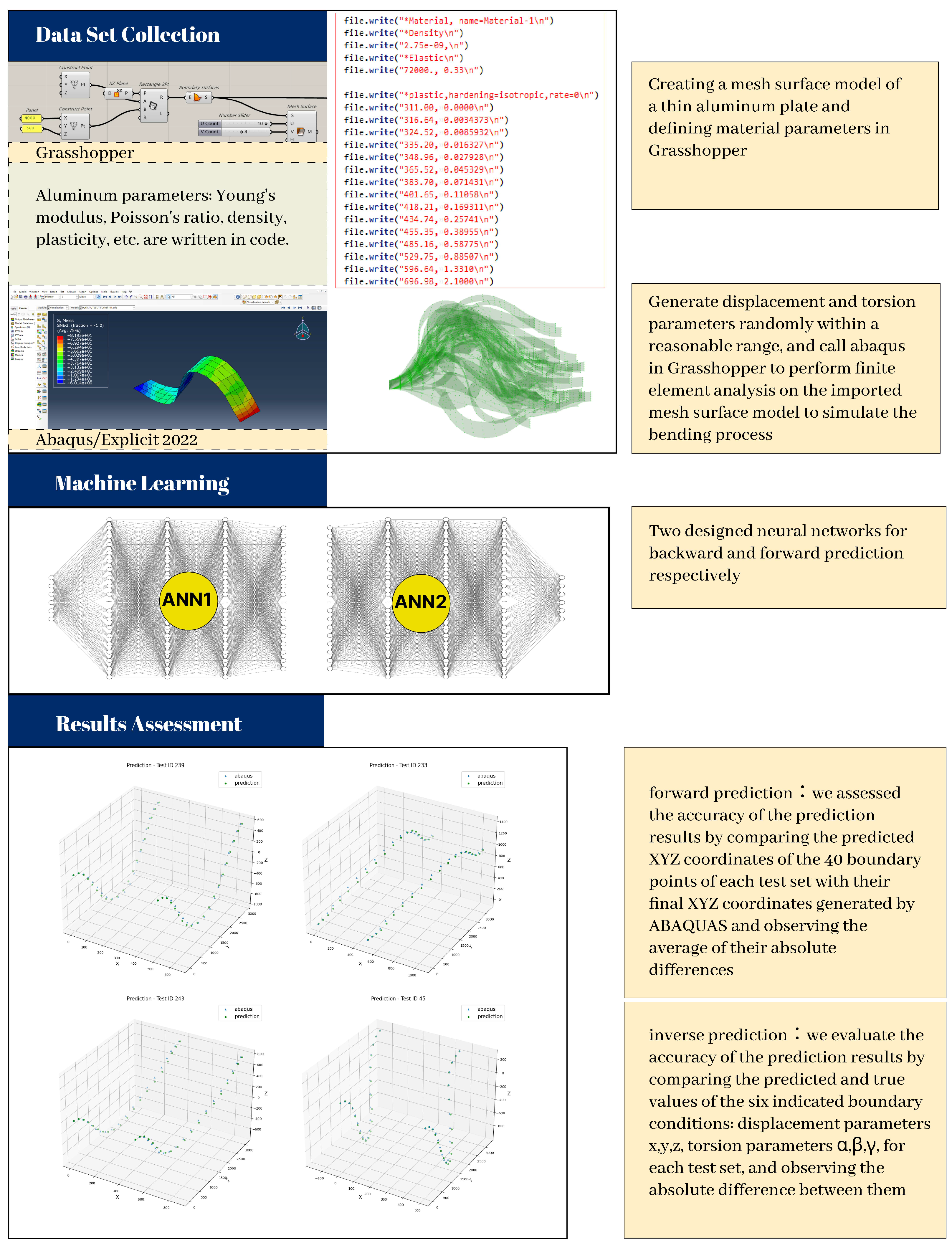
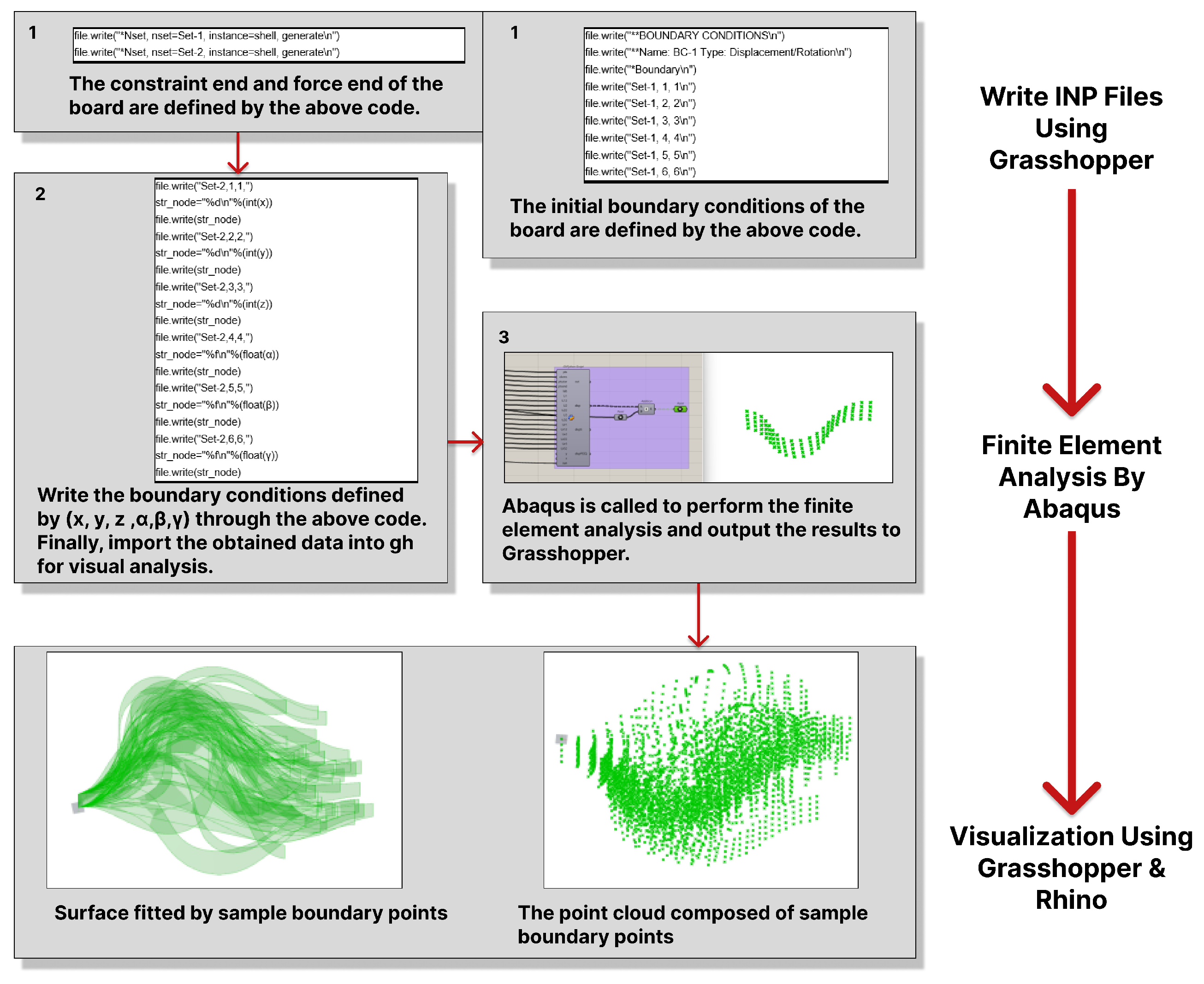
3.1. Data Collection

Based on the sizes of the set of aluminum plates, a mesh surface was established in Grasshopper 1.0.0008, and realistic aluminum parameters were given to it (Young’s modulus of 7.2 × 4 N/mm², Poisson’s ratio of 0.33, density of 2.75 × 3 kg/m³, and plasticity table of aluminum).

As shown in Figure 10a, the rectangular plate was divided into a 5*20 grid (short and long edges were divided into 5 and 20 equal parts, respectively). One end of the rectangular plate was hinged and fixed, and boundary conditions were imposed on the other end. Based on (6) and (7), the six-degree-of-freedom parameters of the displacement and Euler angles are used to describe the displacement $\overrightarrow{d}$ and torsion $Ro{t}_{xyz}$ of the plate edge. Therefore, all boundary conditions can be simplified to $(x,y,z,\alpha ,\beta ,\gamma )$ motion parameters:

$$\begin{array}{c}\hfill \overrightarrow{d}=\overrightarrow{x}+\overrightarrow{y}+\overrightarrow{z}\end{array}$$

(6)

$$\begin{array}{c}\hfill Ro{t}_{xyz}=Ro{t}_x\left(\alpha \right)·Ro{t}_y\left(\beta \right)·Ro{t}_z\left(\gamma \right)\end{array}$$

(7)

The state of the ideal plate does not exist in practice, and the direction of buckling deformation caused by force is random, which generates noise for subsequent machine learning. To solve this problem, we removed the plate from the entirely ideal horizontal state and introduced a 1‰ deformation as a controlled imperfection, which can simulate the initial conditions that may occur in practical applications, making the machine learning model better understand and predict the deformation behavior of the plate (Figure 10b).

As shown in Figure 11, the defined mesh with initial defects and boundary conditions was written into an INP file using Grasshopper 1.0.0008, which generated 3000 sets of samples. Abaqus 2022 was then used to perform the finite element analysis. We used the Abaqus Explicit Solver to solve the quasi-static problem. The load was applied using a smooth-step amplitude, where it gradually increased from 0 to 1 over a time range of 0.00001 to 6.0 s. The results were output to Grasshopper 1.0.0008, where the 3000 sets of results were analyzed (including the final displacement at each point, the magnitude of the stresses, the PEEQ value, etc.), and the data format was adapted. Finally, the generated point cloud was visualized using Grasshopper 1.0.0008 and Rhino 8.6.

We took the two boundary lines of the plate as the observation objects and output the following:

• The displacement components (x, y, z) of the points on the two corresponding boundary lines.
• The bending of the plate, represented by the displacement component along the z-axis of the points at the boundary line.
• The twist angle, represented by the twist angle of the cross-sectional line that forms a curved surface through two boundary lines.

It is worth noting that when materials are subjected to force, plastic deformation is an irreversible change that occurs after reaching their elastic limit, and buckling is the main mode of failure for bending structures. The PEEQ (Plastic Strain Equivalent Peak) indicator included in the dataset helps determine whether the material has undergone plastic deformation. When the PEEQ value is greater than zero, it indicates that parts of the model have yielded. We trained the neural network using the PEEQ value to predict whether the material could achieve yield-free bending under specific boundary conditions.

At the same time, we considered the impact of different displacement paths on the experimental results. We controlled each pair of comparison groups to experience different paths but with the same absolute displacement and total torsion angle, and then analyzed the displacement results at 20 equidistant points on the final plate median to compare the differences between the two (Figure 12). The results showed a difference of 4% (less than 20 mm).

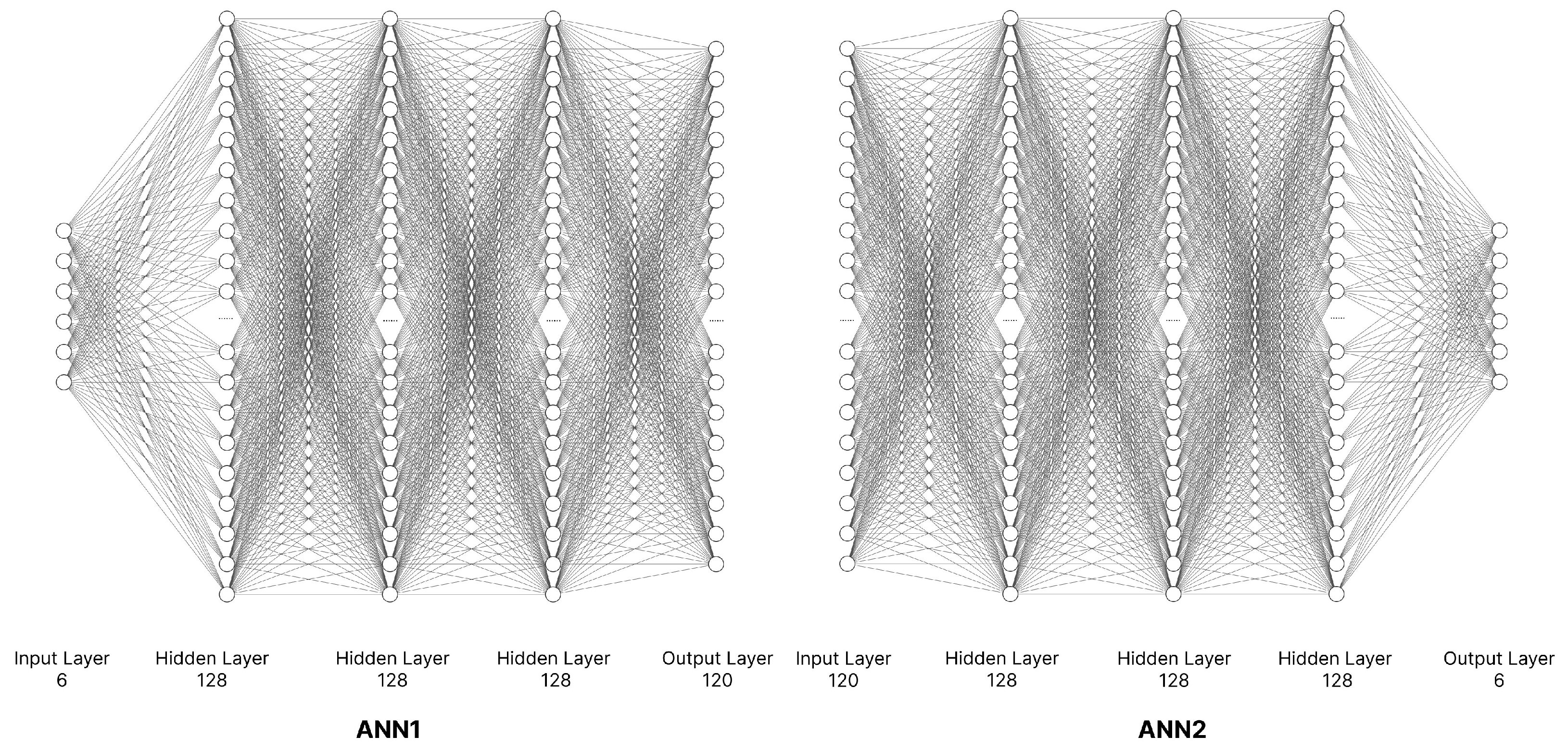
3.2. The Neural Network

In this step, we used neural networks to establish the connection between the deformation and boundary conditions of the thin aluminum plate. Two designed neural networks were used for reverse prediction and forward prediction, respectively. The forward prediction neural network predicts the node positions of the thin aluminum plate shape based on the given boundary conditions. The reverse prediction neural network predicts the possible boundary conditions that cause the shape based on the node position of the thin aluminum plate shape. These two neural networks complement each other and can provide bidirectional predictions of the connection between the shape and deformation conditions of the thin aluminum plate.

3.2.1. Dataset

The dataset contained 3000 samples representing different combinations of deformation and boundary conditions (Figure 13), with 2400 random samples used as the training set and the remaining 600 used as the test set.

3.2.2. Basic Neural Network Architecture

The changes in the aluminum plates conform to the corresponding mechanical laws and can be fitted with correlation functions. Therefore, in this study, a five-layer ANN network structure with three hidden layers was adopted for learning, as shown in Figure 14. The structures of the two neural networks established for forward and reverse predictions were similar. Both were composed of one input layer, three hidden layers, and one output layer, with 128 hidden neurons, activated using the ReLU function.

The input data came from an XLS file containing information on 40 coordinate points, which were transformed into 120 numerical inputs corresponding to the $x,y$, and z coordinates of each point. Additionally, to ensure the stability and accuracy of model training, we normalized the input data for displacement $(x,y,z)$ and torsion $(\alpha ,\beta ,\gamma )$ under boundary conditions.

The forward neural network finds the position of the recorded shape nodes through the input deformation conditions, and the input layer receives a six-dimensional vector $\overrightarrow{s}$ representing the boundary conditions:

$$\begin{array}{c}\hfill \overrightarrow{s}=(x,y,z,\alpha ,\beta ,\phi )\end{array}$$

(8)

The output has 120 values representing the final points of 40 equidistant points (20 on one side) on both boundary lines of the aluminum plate:

$$\begin{array}{c}\hfill p_i=(x_{pi},y_{pi},z_{pi})\\ \hfill *i=1,2,\dots ,39,40\end{array}$$

(9)

The reverse neural network infers the corresponding deformation conditions by inputting the node positions of the recorded shapes. A total of 120 values representing the node positions of the recorded shapes are input to the input layer, and 6 values representing the boundary conditions are output.

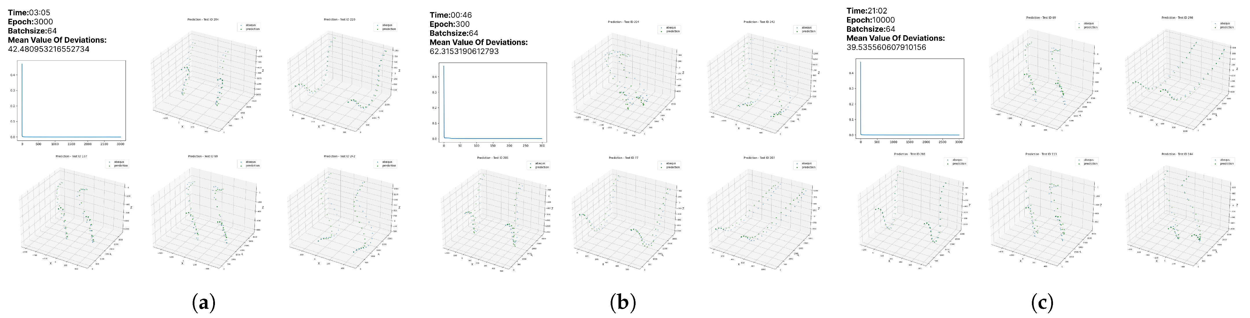
3.2.3. Model Training

As can be seen in Figure 13, there was a significant difference in the numerical domain between $x,y,$ and z, which represent displacement, and $\alpha$, $\beta$, and $\gamma$, which represent torsion. Therefore, we used normalized data preprocessing to map the variables from different numerical domains to the [0,1] interval, transforming different features to the same order of magnitude to ensure that scale differences between different features did not adversely affect model training. Additionally, we shuffled the dataset to reduce bias introduced by the order of data generation and enhance the model’s generalization ability.

We used the mean squared error (MSE) as the loss function of the neural networks and the stochastic gradient method Adam optimizer to optimize the learning rate [42].

To confirm the fit of our neural network models to the training data, we compared the neural network models with different parameters. For all neural network models, we compared the effects of different batch sizes and training periods on the fit. We compared the gradient descent of each model. Figure 15a–c summarize the results.

After comprehensive consideration of time and the fitting effect, we used a batch size of 64, a learning rate of ${10}^{-3}$, and early stopping on a validation set with a patience of 3000 epochs.

Table 1. Key parameters for training neural networks.

Hyperparameter	Value
Learning Rate	1.00 $\times {10}^3$
Epochs	3000
Loss Function	Mean squared error (MSE)
Activation Function	ReLU
Optimizer	Adam optimizer
Batch Size	64

lists the hyperparameters of our model. The model was implemented on Pytorch and programmed in Python.

The model trained with the selected parameters performed exceptionally well, processing a set of samples in just 0.06 s. In contrast, Abaqus 2022 required 38 s to process the same set, making the neural network 633 times faster and highlighting the high efficiency of this method.

4. Results

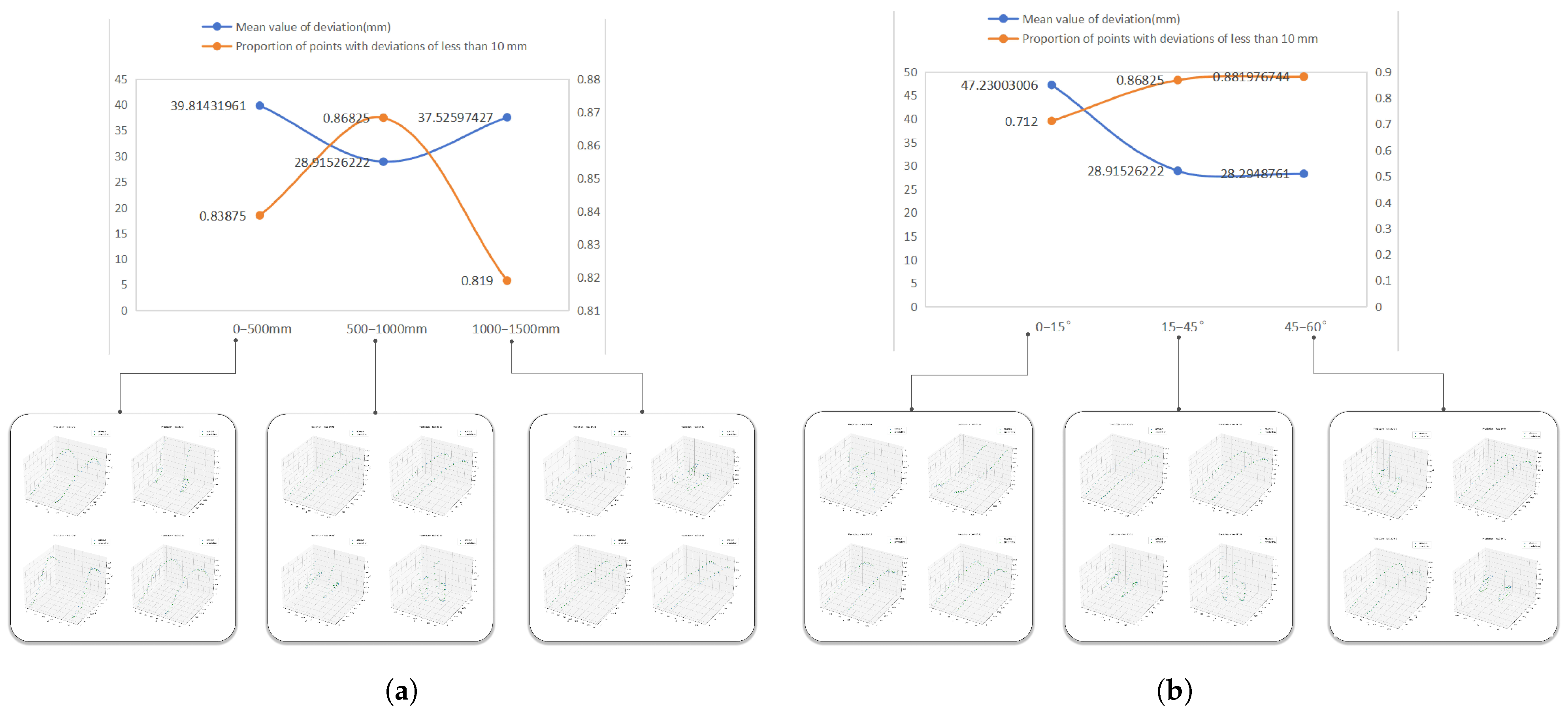
4.1. Forward Bending Shape Prediction

By testing the forward prediction of curved geometries based on given boundary conditions, the accuracy of predicting whether they were yielded reached 90%; for morphological prediction, in the nodes of the neural network predicting deformation, 46.29% of the predicted samples had an error of less than 10 mm, with an average error of 12.71 mm, which was only 0.602% of the plate’s length. Some prediction results and biases are shown in Figure 16.

We further investigated the average deviation and relative accuracy by dividing the input translation distance and torsion angle into different intervals. The translation distance was divided into 0–500 mm, 500–1000 mm, and 1000–1500 mm, and the torsion angle was divided into 0–15°, 15–45°, and 45–60°. According to the experimental data, the average deviation was the lowest when the translation distance was between 500 and 1000 mm and the torsion angle was between 45 and 60° (Figure 17, Figure 18 and Figure 19).

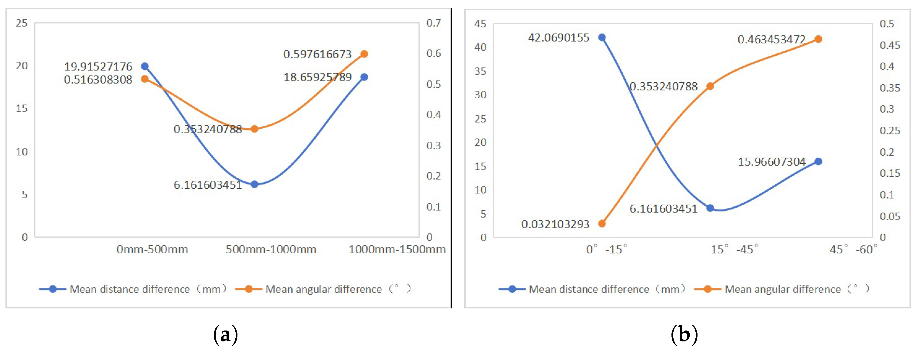
4.2. Reverse Boundary Condition Prediction

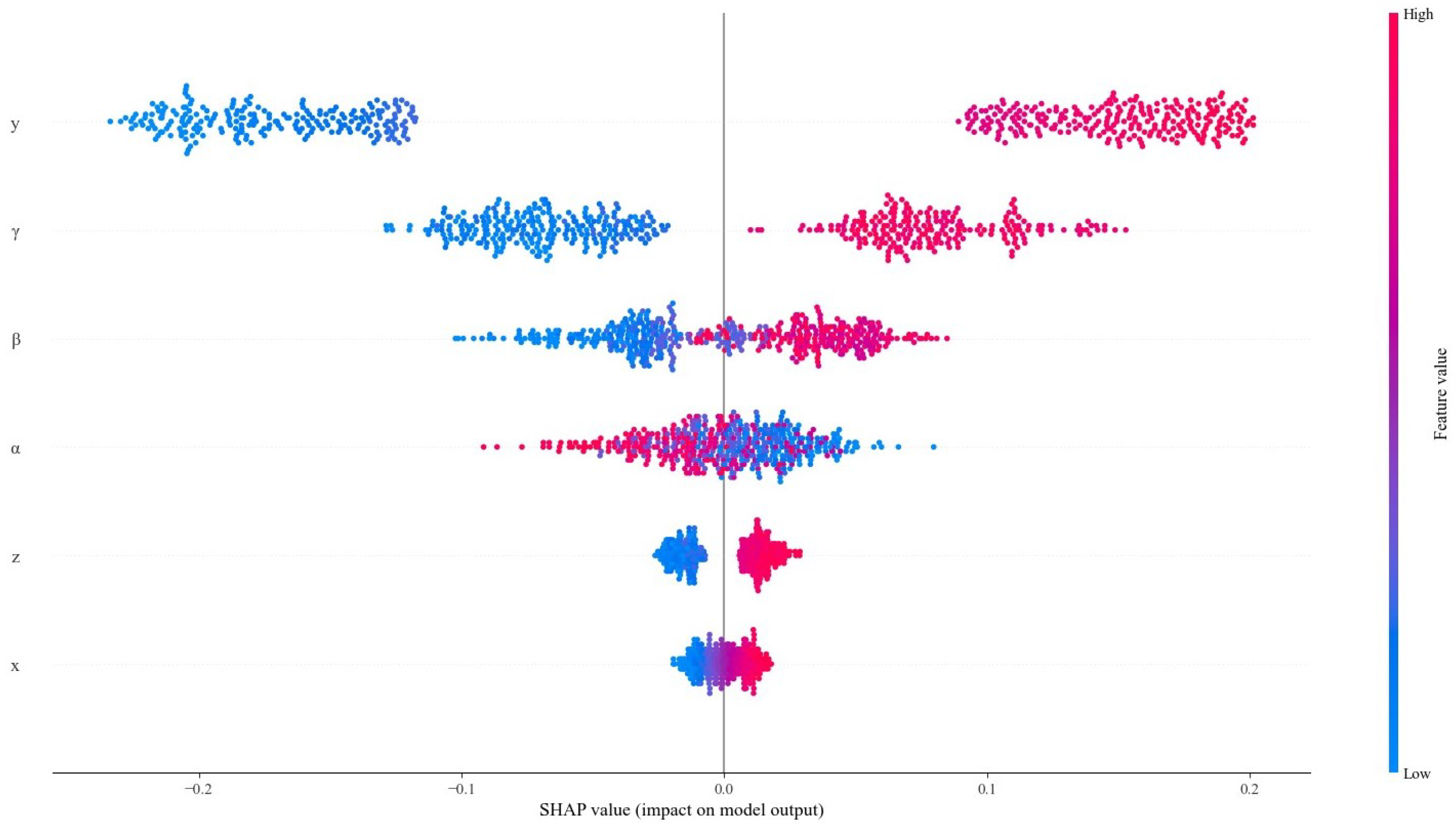
The reverse prediction model can extract 40 boundary points based on a given geometric shape and use the coordinates (x, y, z) of these points to predict whether the shape can be manufactured by active bending, that is, no fracture occurs during the bending process. Finally, the model also provides the results of the six boundary conditions closest to the given geometric shape.

In the test of the reverse prediction of possible boundary conditions, the average error of the neural networks predicting the initial translation was 3.273 mm, accounting for only 0.49% of the average range of all sampled translations, and the average error angle was 0.488°, accounting for only 4.7% of the average range of all sampled angles. Figure 20 shows the prediction results.

The results show that the proposed method and tool achieved good accuracy in inferring initial conditions and predicting deformation.

We divided the input translation distance and torsion angle into different intervals according to the method described in Section 4.1 and further examined the average deviation and relative accuracy. Through experimental data, it can be seen that the best fitting results were achieved when the torsion angle was between 15° and 45° and the translation distance was between 500 mm and 1000 mm, taking into account the average error distance and the average error angle (Figure 21).

4.3. SHAP Analysis

We applied SHAP (SHapley Additive exPlanations) to assign importance values to each feature of the model, thereby explaining the model’s prediction process. In Figure 22, the further a point is from the centerline, the greater the impact of that feature on the model output. The features are vertically arranged in the graph in order of decreasing influence, with the features at the top having a greater overall impact on the model output, while those at the bottom have a smaller impact. The distribution of points for the top feature (y) shows a significant amount of both positive and negative effects, indicating that its variations have a substantial impact on the outcomes of the model’s predictions. The distribution of points for the middle feature (e.g., $\alpha$) is more concentrated, with a relatively smaller impact. The bottom features (e.g., x) have the least impact on the model, and most of their impacts are close to zero, indicating that these features contribute less to the model’s prediction (Figure 22).

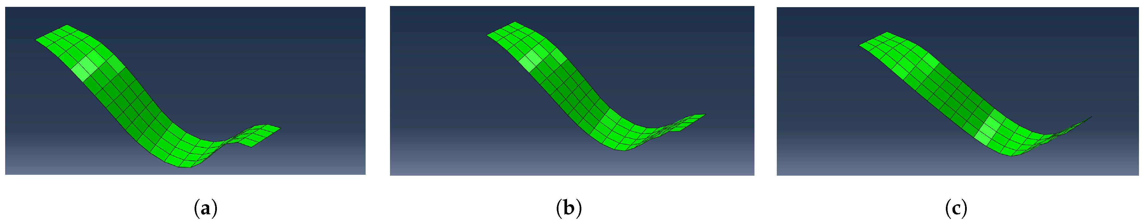
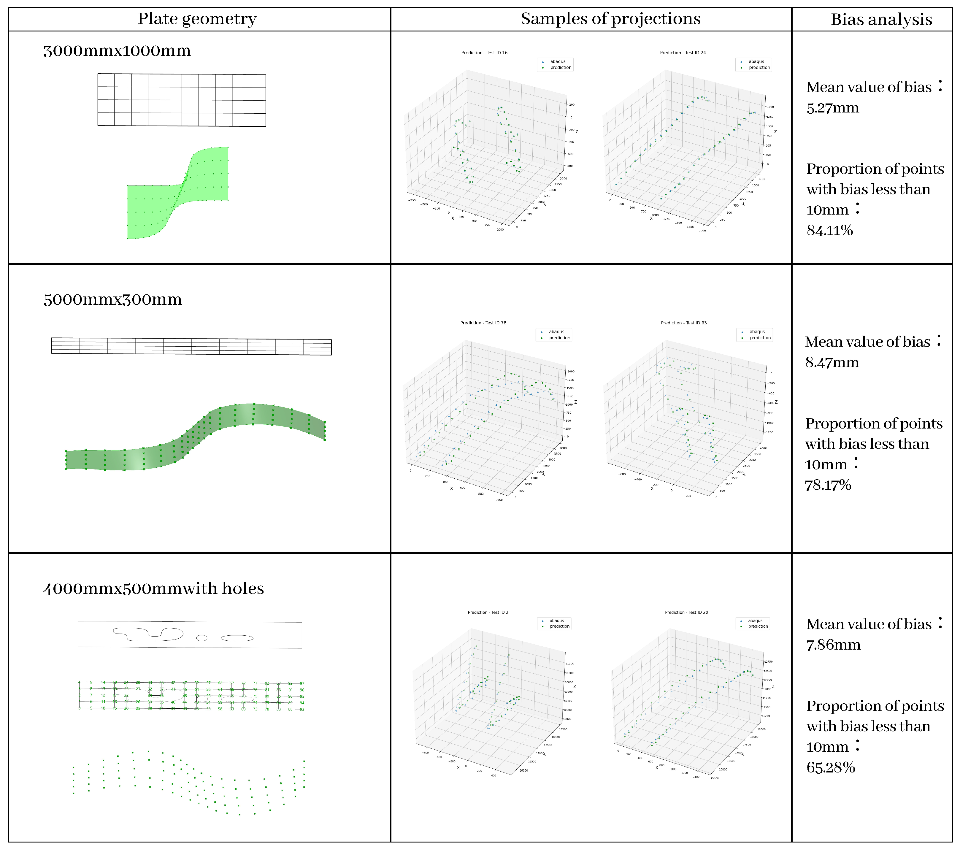
4.4. Test with Different Geometries

To verify the generalizability of this method, we conducted experiments with plates of different sizes, setting up plates of 5000 mm × 300 mm and 3000 mm × 1000 mm. By using 500 small samples for transfer learning based on the original model, we achieved good results: the mean bias for the 3000 mm × 1000 mm plate was 5.27 mm, with 84.11% of the points having a bias less than 10 mm, and the mean bias for the 5000 mm × 300 mm plate was 8.47 mm, with 78.17% of the points having a bias less than 10 mm. For plates with central holes, we imported the plate into Rhino 8.6 and converted it into a mesh surface. Then, we took all the mesh points on the boundary and repeated the above method to train the model, which predicted the final shape quite accurately: the mean bias for the 4000 mm × 500 mm plate with holes was 7.86 mm, with 65.28% of the points having a bias less than 10 mm (Figure 23).

4.5. Transfer Learning

We employed the transfer learning method using a model pretrained on simulated data to predict the data from actual thin-plate bending experiments. Specifically, we used two robotic arms to perform multiple bending operations on a 1000 mm × 125 mm, 0.8 mm thick aluminum plate and scanned its shape after bending (Figure 24). We recorded the final positions of 40 equidistant points along its edge. Through Grasshopper 1.0.0008, we mapped the collected coordinate points onto the coordinate system defined by the simulation dataset, arranging them in their original order to ensure data consistency and comparability. We then fine-tuned the pre-trained model with this dataset, training with a lower learning rate and achieving good fitting effects after just a few epochs (Figure 25).

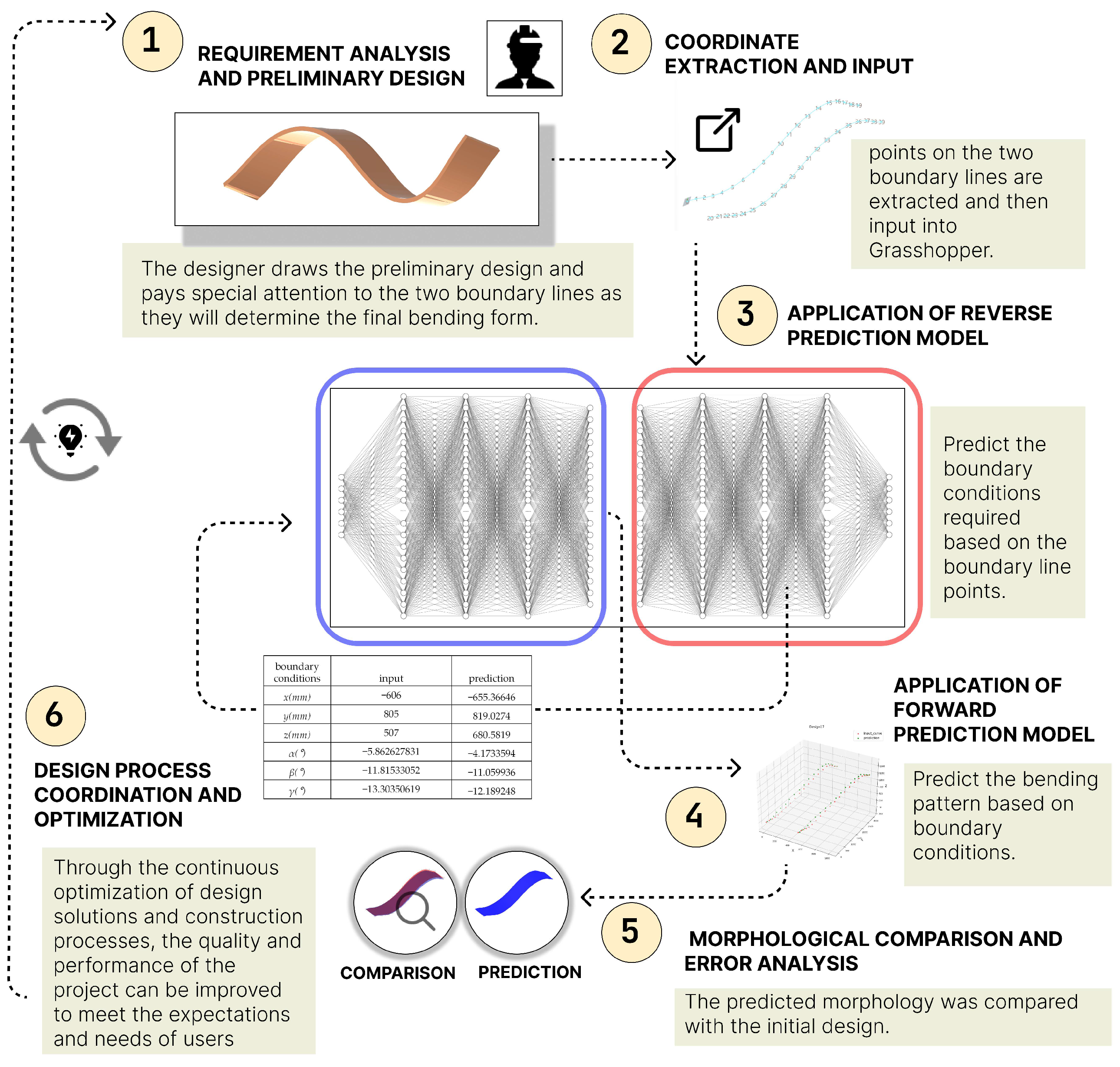
4.6. Application of Neural Networks to the Design Process

We applied the network to a specific design to optimize the design process of active-bending structures. The optimization process of active-bending structure design is divided into the following phases: (1) requirement analysis and preliminary design; (2) coordinate extraction and input; (3) application of the reverse prediction model; (4) application of the forward prediction model; (5) morphological comparison and error analysis; and (6) design process coordination and optimization.

Firstly, according to the specific needs of the project (understanding the function of the final product, consideration of structural requirements, and analysis of material properties), the morphology of the thin plate to be bent is determined. The designer draws the preliminary design form through sketching or modeling software and pays special attention to the two boundary lines of the sheet, as they determine the final bending form.

After determining the design form, the point coordinates of 40 equidistant boundary points on the two boundary lines need to be extracted. This can be performed using design software (e.g., AutoCAD 2022) or modeling software. These coordinates of the boundary line points are then input into Grasshopper 1.0.0008.

Next, the already trained reverse prediction model is utilized. This model predicts the boundary conditions (displacement and torsion) required to realize the morphology based on the coordinates of the input boundary line points. At the same time, the reverse prediction model excludes conditions that may lead to bending or non-compliance with design requirements, providing reasonable input parameters for the forward prediction that follows.

Once the appropriate boundary conditions are obtained by the reverse prediction model, these parameters are input into the forward prediction model. The forward prediction model predicts the bending pattern the sheet will exhibit based on these boundary conditions. This predicted morphology is described by 40 boundary equipartition points, which helps understand the bending of the thin plate more accurately.

After obtaining the predicted morphology, it is compared with the initial design morphology to quantify the difference between the two using the superposition of morphologies, difference set operations, and distance analysis. By calculating the average error (45 mm in Figure 26), the degree of similarity between the predicted morphology and the designed morphology can be assessed.

Based on the results of the morphological comparison and error analysis, designers need to adjust the boundary conditions or optimize the prediction model to reduce the difference between the predicted morphology and the designed morphology. Through iteration and optimization, the designer can gradually approach the design goal and achieve the optimal design of the active-bending structure.

Effective interaction and timely feedback between the design and construction phases of active bending are achieved throughout the process, helping to reduce design changes and rework, lower project costs, and improve the execution and resilience of the construction team to ensure that the project can be carried out smoothly according to the intended plan. Finally, through the continuous optimization of design solutions and construction processes, the quality and performance of the project can be improved to meet the expectations and needs of users.

5. Conclusions

This article proposes a method that combines finite element analysis and machine learning to predict the deformation morphology and boundary conditions of thin aluminum plates in bending and discusses its accuracy. The experiment uses the input of 3000 finite element analysis results to achieve fast and accurate predictions. At the same time, not only is forward bending prediction achieved but also reverse prediction of possible boundary conditions is achieved. Additionally, we validate the method on plates of different geometries, thereby proving its generalizability.

Compared to traditional engineering methods, the proposed method provides a more direct way to learn from materials through machine learning. At the same time, we can adjust material parameters and sample generation strategies to adapt the model to the characteristics and behaviors of different materials, thereby enabling the prediction and analysis of complex materials. We can combine Abaqus 2022 to create a large number of complex bending samples with different geometries, material combinations, and loading conditions in the sample generation stage, and by adjusting the material parameters of composites in Abaqus 2022, combining the material models, etc., we can more accurately simulate the anisotropy and nonlinear stress-strain relationship of composites and calibrate the material parameters using experimental data. Subsequently, by using parametric modeling techniques, we can automate the generation of a series of samples covering various environmental conditions that composite materials may encounter. Utilizing the large number of bending samples generated, we can train models to predict the performance and behavior of complex materials under different conditions, providing an inspiring approach for analyzing the behavior of complex materials.

The experiment only considers quasi-static processes, but in the future, models that can predict dynamic processes can be trained using a series of incremental step states (Figure 27a) as training samples. At the same time, the current study uses PEEQ values to ensure that the plate has not yielded, and in the future, a model that can predict the stress distribution on the plate will be trained using stress values at various points as samples (Figure 27b).

Although this method is very effective, this study also highlights some limitations. Especially in extreme cases, predictions may be insufficient, and complex material properties (such as anisotropy) have not been fully considered. Future research will focus on conducting more actual physical bending tests to verify the model’s predictive capabilities. At the same time, we look forward to using artificial intelligence as an important tool for understanding materials and manufacturing processes to better study the behavior and performance of materials.

References

1. Gengnagel, C.; Alpermann, H.; Lafuente, E. Active Bending in Hybrid Structures. In FORM-RULE| RULE-FORM; Innsbruck University Press: Innsbruck, Austria, 2013; pp. 12–27. [Google Scholar]
2. Lienhard, J.; Alpermann, H.; Gengnagel, C.; Knippers, J. Active bending, a review on structures where bending is used as a self-formation process. Int. J. Space Struct. 2013, 28, 187–196. [Google Scholar] [CrossRef]
3. Lienhard, J.; Gengnagel, C. Recent developments in bending-active structures. In Proceedings of the IASS Annual Symposia, International Association for Shell and Spatial Structures (IASS), Boston, MA, USA, 16 July 2018; Volume 2018, pp. 1–8. [Google Scholar]
4. Nicholas, P.; Tamke, M. Computational strategies for the architectural design of bending active structures. Int. J. Space Struct. 2013, 28, 215–228. [Google Scholar] [CrossRef]
5. Schleicher, S.; Rastetter, A.; La Magna, R.; Schönbrunner, A.; Haberbosch, N.; Knippers, J. Form-finding and design potentials of bending-active plate structures. In Modelling Behaviour: Design Modelling Symposium, 2015; Springer: Cham, Switzerland, 2015; pp. 53–63. [Google Scholar]
6. Lienhard, J. Bending-Active Structures: Form-Finding Strategies Using Elastic Deformation in Static and Kinetic Systems and the Structural Potentials Therein. 2014. Available online: https://elib.uni-stuttgart.de/handle/11682/124 (accessed on 1 January 2020).
7. Designboom, n. Uni. of Calgary Team Designs, Builds, & Installs Experimental Pavilion. Available online: https://www.designboom.com/architecture/university-of-calgary-evds-experimental-pavilion-block-week-11-07-2015/ (accessed on 1 January 2020).
8. Alpermann, H.; Lafuente Hernández, E.; Gengnagel, C. Case-studies of arched structures using actively-bent elements. In Proceedings of the IASS-APCS Symposium: From Spatial Structures to Space Structures, Seoul, Republic of Korea, 21–24 May 2012. [Google Scholar]
9. Laccone, F.; Malomo, L.; Pietroni, N.; Cignoni, P.; Schork, T. Integrated computational framework for the design and fabrication of bending-active structures made from flat sheet material. In Structures; Elsevier: Amsterdam, The Netherlands, 2021; Volume 34, pp. 979–994. [Google Scholar]
10. Puystiens, S.; Van Craenenbroeck, M.; Van Hemelrijck, D.; Van Paepegem, W.; Mollaert, M.; De Laet, L. Implementation of bending-active elements in kinematic form-active structures-Part I: Design of a representative case study. Compos. Struct. 2019, 216, 436–448. [Google Scholar] [CrossRef]
11. Brancart, S.; De Laet, L.; Vergauwen, A.; De Temmerman, N. Transformable active bending: A kinematical concept. Mob. Rapidly Assem. Struct. IV 2014, 136, 171–182. [Google Scholar]
12. De Laet, L.; Veenendaal, D.; Van Mele, T.; Mollaert, M.; Block, P. Bending incorporated: Designing tension structures by integrating bendingactive elements. In Proceedings of the TensiNet 2013 Symposium [RE] THINKING Lightweight Structures, Istanbul, Turkey, 8–10 May 2013; pp. 251–256. [Google Scholar]
13. Vorstermans, R.L.; van Wijk, J.; Teuffel, P.; Habraken, A.P.; Houtman, R. Integration of form-finding, analysis process and production of a bending-active textile hybrid into one model. In Proceedings of the 6th Tensinet Symposia, Milan, Italy, 3–5 June 2019; pp. 123–134. [Google Scholar]
14. Alpermann, H.; Gengnagel, C. Restraining actively-bent structures by membranes. In Proceedings of the Textiles Composites and Inflatable Structures VI: Proceedings of the VI International Conference on Textile Composites and Inflatable Structures, Barcelona, Spain, 9–11 October 2013; CIMNE: Barcelona, Spain, 2013; pp. 62–70. [Google Scholar]
15. Lienhard, J.; La Magna, R.; Knippers, J. Form-finding bending-active structures with temporary ultra-elastic contraction elements. Mob. Rapidly Assem. Struct. IV 2014, 107, 115. [Google Scholar]
16. D’Amico, B.; Zhang, H.; Kermani, A. A finite-difference formulation of elastic rod for the design of actively bent structures. Eng. Struct. 2016, 117, 518–527. [Google Scholar] [CrossRef]
17. Liuti, A.; Mazzola, C.; Zanelli, A. Where design meets construction: A review of bending active structures. In Proceedings of the IASS Annual Symposia, International Association for Shell and Spatial Structures (IASS), Boston, MA, USA, 16 July 2018; Volume 2018, pp. 1–8. [Google Scholar]
18. Fleischmann, M.; Menges, A. ICD/ITKE Research Pavilion: A case study of multi-disciplinary collaborative computational design. In Computational Design Modelling: Proceedings of the Design Modelling Symposium Berlin, 2011; Springer: Berlin/Heidelberg, Germany, 2011; pp. 239–248. [Google Scholar]
19. Menges, A. Integrative design computation for advancing wood architecture. In Advancing Wood Architecture; Routledge: London, UK, 2016; pp. 97–109. [Google Scholar]
20. Menges, A.; Knippers, J. Architecture Research Building: ICD/ITKE 2010–2020; Birkhäuser: Basel, Switzerland, 2020. [Google Scholar]
21. archDaily. ICD-ITKE Research Pavilion 2015-16/ICD-ITKE University of Stuttgart, Germany. Available online: https://www.archdaily.cn/cn/787034/icd-itke-yan-jiu-zhan-ting-2015-16-icd-itke-de-guo-si-tu-jia-te-da-xue (accessed on 1 January 2020).
22. Brew, J.; Brotton, D. Non-linear structural analysis by dynamic relaxation. Int. J. Numer. Methods Eng. 1971, 3, 463–483. [Google Scholar] [CrossRef]
23. Cuvilliers, P.; Yang, J.R.; Coar, L.; Mueller, C. A comparison of two algorithms for the simulation of bending-active structures. Int. J. Space Struct. 2018, 33, 73–85. [Google Scholar] [CrossRef]
24. Pone, S. Digital tools and experimentations for structures realised with the active bending. Techne-J. Technol. Archit. Environ. 2017, 306–312. [Google Scholar] [CrossRef]
25. Senatore, G.; Piker, D. Interactive real-time physics: An intuitive approach to form-finding and structural analysis for design and education. Comput.-Aided Des. 2015, 61, 32–41. [Google Scholar] [CrossRef]
26. Hairer, E.; Hochbruck, M.; Iserles, A.; Lubich, C. Geometric numerical integration. Oberwolfach Rep. 2006, 3, 805–882. [Google Scholar] [CrossRef]
27. La Magna, R.; Schleicher, S.; Knippers, J. Bending-active plates. Adv. Archit. Geom. 2016, 2016, 170–187. [Google Scholar]
28. Bauer, A.M.; Längst, P.; La Magna, R.; Lienhard, J.; Piker, D.; Quinn, G.; Gengnagel, C.; Bletzinger, K.U. Exploring software approaches for the design and simulation of bending active systems. In Proceedings of the IASS Annual Symposia, International Association for Shell and Spatial Structures (IASS), Boston, MA, USA, 16 July 2018; Volume 2018, pp. 1–8. [Google Scholar]
29. Larson, M.G.; Bengzon, F. The Finite Element Method: Theory, Implementation, and Applications; Springer Science & Business Media: Boston, NY, USA, 2013; Volume 10. [Google Scholar]
30. Norrie, D.H.; De Vries, G. The Finite Element Method: Fundamentals and Applications; Academic Press: New York, NY, USA, 2014. [Google Scholar]
31. Singh, K.; Kapania, R.K. Accelerated optimization of curvilinearly stiffened panels using deep learning. Thin-Walled Struct. 2021, 161, 107418. [Google Scholar] [CrossRef]
32. Veeramachaneni, K.; Peram, T.; Mohan, C.; Osadciw, L.A. Optimization using particle swarms with near neighbor interactions. In Proceedings of the Genetic and Evolutionary Computation—GECCO 2003: Genetic and Evolutionary Computation Conference, Chicago, IL, USA, 12–16 July 2003; Proceedings, Part I. Springer: Berlin/Heidelberg, Germany, 2003; pp. 110–121. [Google Scholar]
33. Zadeh, L.A. Fuzzy logic, neural networks, and soft computing. In Fuzzy Sets, Fuzzy Logic, and Fuzzy Systems: Selected Papers by Lotfi A Zadeh; World Scientific: London, UK, 1996; pp. 775–782. [Google Scholar]
34. Maier, H.R.; Dandy, G.C. Neural networks for the prediction and forecasting of water resources variables: A review of modelling issues and applications. Environ. Model. Softw. 2000, 15, 101–124. [Google Scholar] [CrossRef]
35. Fateh, A.; Hejazi, F. Experimental testing of variable stiffness bracing system for reinforced concrete structure under dynamic load. J. Earthq. Eng. 2022, 26, 1416–1437. [Google Scholar] [CrossRef]
36. Bouman, K.L.; Xiao, B.; Battaglia, P.; Freeman, W.T. Estimating the material properties of fabric from video. In Proceedings of the IEEE International Conference on Computer Vision, Sydney, Australia, 1–8 December 2013; pp. 1984–1991. [Google Scholar]
37. Davis, A.; Bouman, K.L.; Chen, J.G.; Rubinstein, M.; Durand, F.; Freeman, W.T. Visual vibrometry: Estimating material properties from small motion in video. In Proceedings of the IEEE Conference on Computer Vision and Pattern Recognition, Boston, MA, USA, 7–12 June 2015; pp. 5335–5343. [Google Scholar]
38. Wang, H.; Yang, Y. Descent methods for elastic body simulation on the GPU. ACM Trans. Graph. (TOG) 2016, 35, 1–10. [Google Scholar] [CrossRef]
39. Rodriguez-Pardo, C.; Prieto-Martin, M.; Casas, D.; Garces, E. How will it drape like? Capturing fabric mechanics from depth images. In Computer Graphics Forum; Wiley Online Library: Hoboken, NJ, USA, 2023; Volume 42, pp. 149–160. [Google Scholar]
40. Gavriil, K.; Guseinov, R.; Pérez, J.; Pellis, D.; Henderson, P.; Rist, F.; Pottmann, H.; Bickel, B. Computational design of cold bent glass façades. ACM Trans. Graph. (TOG) 2020, 39, 1–16. [Google Scholar] [CrossRef]
41. Mojtabaei, S.M.; Becque, J.; Hajirasouliha, I.; Khandan, R. Predicting the buckling behaviour of thin-walled structural elements using machine learning methods. Thin-Walled Struct. 2023, 184, 110518. [Google Scholar] [CrossRef]
42. Kingma, D.P. Adam: A method for stochastic optimization. arXiv 2014, arXiv:1412.6980. [Google Scholar]
Figure 1. Self-strutted geodesic Plydome by Buckminster Fuller. Reprinted from ref. [3].
Electronics 14 00503 g001
Figure 2. The exterior of the ‘experimental pavilion’ [7].
Electronics 14 00503 g002
Figure 3. The span of the hemisphere is 7.3 m and is made of marine plywood with a thickness of 6.4 mm. Reprinted from ref. [3].
Electronics 14 00503 g003
Figure 4. The span of the hemisphere is 7.3 m and is made of marine plywood with a thickness of 6.4 mm. ©ICD/ITKE University of Stuttgart.
Electronics 14 00503 g004
Figure 5. Physical/digital test of elastic plywood bending behavior (a) and simulation of system behavior (b) in the 2015-16 ICD-ITKE research pavilion project. Reprinted with permission from ref. [18]. Copyright 2011 Springer.
Electronics 14 00503 g005
Figure 6. 2015-16 ICD-ITKE research pavilion, ICD-ITKE Germany University of Stuttgart. (a) Aerial View; (b) Human Perspective View. ©ICD/ITKE University of Stuttgart [21].
Electronics 14 00503 g006
Figure 7. In the 2015-16 ICD-ITKE research pavilion project, architects and engineers collaborated across disciplines to deeply analyze natural segmented shell-shaped structures. (a) Architectural components were made from extremely thin wooden slats. By leveraging the anisotropic properties of wood, these slats were subjected to a specific compounding process to achieve deformation within a certain radius; (b) The project, starting from the analysis of the construction morphology of sand dollars, developed a manufacturing technique that allows for the elastic bending of double-layered segmentally laminated veneer lumber. ©ICD/ITKE University of Stuttgart.
Electronics 14 00503 g007
Figure 8. The mesh surface model of the thin aluminum plate was created in Grasshopper 1.0.0008, and finite element analysis was conducted in Abaqus 2022 to construct the dataset.
Electronics 14 00503 g008
Figure 9. Sample sets of rectangular aluminum plates, each described by 100 grid points.
Electronics 14 00503 g009
Figure 10. (a) The simulation in Abaqus 2022; (b) Creating a certain initial displacement in the experiment.
Electronics 14 00503 g010
Figure 11. Data generation and processing.
Electronics 14 00503 g011
Figure 12. A comparison group with the same total displacement and total torsion angle but different paths.
Electronics 14 00503 g012
Figure 13. The data were stored in XLS format. Each column represents a training sample. Row 1 is the serial number of the sample, rows 2–7 record the boundary conditions, row 8 represents whether it is yielded or not (1 indicates no yield), and rows 9–48 are the coordinate records of the sampling points on the two boundary lines, representing the deformation of the aluminum plate according to the order of the initial grid of the plate.
Electronics 14 00503 g013
Figure 14. ANN architectures in this research.
Electronics 14 00503 g014
Figure 15. (a) Effect with a batch size of 64 and 3000 epochs; (b) Effect with a batch size of 64 and 300 epochs; (c) Effect with a batch size of 64 and 10,000 epochs.
Electronics 14 00503 g015
Figure 16. (a) Some prediction results; (b) Proportion of bias in points.
Electronics 14 00503 g016
Figure 17. (a) Keeping the torsion angle in the range of 15–45° and the translation distance in the range of 0–500 mm; (b) Keeping the torsion angle in the range of 15–45°, panning distance in the range of 500–1000 mm; (c) Keeping the torsion angle in the range of 15–45° and the translation distance in the range of 1000–1500 mm.
Electronics 14 00503 g017
Figure 18. (a) Keeping the translation distance in the range of 500–1000 mm and the twist angle in the range of 0–15°; (b) Keeping the translation distance in the range of 500–1000 mm and the twist angle in the range of 15–45°; (c) Keeping the translation distance in the range of 500–1000 mm and the twist angle in the range of 45–60°.
Electronics 14 00503 g018
Figure 19. (a) Forward prediction experiment changing the translation distance interval while maintaining the twist angle in the 15–45° range; (b) Forward prediction experiment changing the twist angle interval while maintaining the translation distance in the 500–1000 mm range.
Electronics 14 00503 g019
Figure 20. Prediction results for ( x , y , z , α , β , γ ) .
Electronics 14 00503 g020
Figure 21. (a) Reverse prediction experiment changing the translation distance interval while maintaining the twist angle in the 15–45° range; (b) Reverse prediction experiment changing the twist angle interval while maintaining the translation distance in the 500–1000 mm range.
Electronics 14 00503 g021
Figure 22. SHAP summary plot based on a subset of samples.
Electronics 14 00503 g022
Figure 23. The experimental results with plates of different shapes.
Electronics 14 00503 g023
Figure 24. (a) Conducting multiple bending experiments on thin plates using a robotic arm; (b) Scanning the final shape and recording the point cloud.
Electronics 14 00503 g024
Figure 25. Transfer learning: Processing the obtained point cloud data and performing transfer learning.
Electronics 14 00503 g025
Figure 26. Application of networks to optimize the design process of active-bending structures.
Electronics 14 00503 g026
Figure 27. (a) Bending increment step; (b) Stress distribution.
Electronics 14 00503 g027