Three-Dimensional Dynamic Positioning Using a Novel Lyapunov-Based Model Predictive Control for Small Autonomous Surface/Underwater Vehicles

Abstract

Small Autonomous Surface/Underwater Vehicles (S-ASUVs) are gradually attracting attention from related fields due to their small size, low energy consumption, and flexible motion. Existing dynamic positioning (DP) control approaches suffer from chronic restrictions that hinder adaptability to varying practical conditions, rendering performance poor. A new three-dimensional (3D) dynamic positioning control method for S-ASUVs is proposed to tackle this issue. Firstly, a dynamic model for the DP control problem considering thrust allocation was established deriving from dynamic models of S-ASUVs. A novel Lyapunov-based model predictive control (LBMPC) method was then designed. Unlike the conventional Lyapunov-based model predictive control (LMPC), this study used multi-variable proportional–integral–derivative (PID) control as the secondary control law, improving the accuracy and rapidity of the control performance significantly. Both the feasibility and stability were rigorously proved. A series of digital experiments using the S-ASUV model under diverse conditions demonstrate the proposed method’s advantages over existing controllers, affirming satisfactory performances for 3D dynamic positioning in complex environments.

1. Introduction

The Earth’s surface is 71% water, with 97% of that being ocean water [1]. Despite this vast coverage, only 23% of the seafloor has been mapped in detail, and even less has been explored using underwater cameras or submersibles [2]. Marine vehicles, such as deep-sea autonomous remote vehicles (ARVs), are increasingly gaining attention in academic and corporate sectors due to their ability to provide secure and economically efficient alternatives to human involvement in marine engineering. DP control of marine vehicles has applications in underwater monitoring, maintenance, operations, rescue, aquaculture, and scientific research. S-ASUVs, in particular, have attracted significant interest due to their compact size, low energy consumption, and flexible motion [3,4].

This research is motivated by the challenges of achieving precise and rapid dynamic positioning for autonomous underwater vehicles (AUVs) in complex and unpredictable underwater environments. These challenges are further compounded by the nonlinearities, intricate hydrodynamic coefficients, and model uncertainties inherent in AUVs [5]. DP traditionally refers to maintaining a vehicle’s desired position and orientation using active thrusters. Recently, it has expanded to include all low-speed maneuvers.

Several control methods have been proposed to address DP challenges. Classical PID controllers and modern model predictive control (MPC) are prominent among these [6,7]. MPC has gained traction due to its optimization-based approach, enabling the explicit handling of constraints during the controller design process. Despite these advantages, traditional MPC designs face limitations in guaranteeing closed-loop stability for nonlinear systems like AUVs, often requiring conservative constraints and linearization techniques [8].

Tube-based MPC approaches have been introduced to improve robustness for autonomous surface vessels, addressing both measurable states and partial states with errors [9]. However, these methods suffer from computational complexity, making them challenging to implement in real time for systems with 3D state spaces and fast dynamics. Additionally, the reliance on state estimation methods like the Luenberger observer may limit performance in scenarios with significant measurement errors.

Alternative strategies have also been explored. Finite-time adaptive DP controllers employing fuzzy supervisory approaches [10] and discrete-time adaptive predictive sliding mode controllers [11] address specific issues such as disturbances and input saturation. While effective in specific cases, these methods often face challenges in handling complex dynamics, reliance on disturbance observers, and sensitivity to model inaccuracies.

LMPC strategies have shown promise for two-dimensional (2D) trajectory tracking problems. For example, Ref. [12] proposed an LMPC scheme with a proportional-derivative (PD) secondary controller, integrating online optimization with conventional PID theory. However, the scheme does not fully exploit PID’s capabilities. Another study introduced a nonlinear LMPC framework with a backstepping secondary control law and contraction constraints for AUVs [13]. Although effective, the backstepping approach struggles with dramatic model uncertainties and remains constrained to 2D applications.

The combination of MPC and PID control methodologies presents an ideal modern solution to DP problems by leveraging robustness and optimization. However, existing studies primarily address 2D trajectory tracking, leaving the more complex 3D DP problem relatively unexplored. Addressing the DP control problem in 3D space, which involves managing six degrees of freedom (surge, sway, heave, roll, pitch, yaw) and significant coupling effects, remains a critical research gap.

This study aims to bridge these gaps by proposing a novel LBMPC method for 3D DP. Unlike conventional LMPC techniques, the proposed method integrates a multi-variable PID controller as the secondary law, significantly improving accuracy and rapidity. It directly incorporates thrust allocation into the optimization framework, eliminating the need for a separate subproblem.

The main contributions of this study are summarized as follows:

(1)

A new 3D dynamic positioning control methodology, i.e., LBMPC, is proposed for S-ASUVs, providing a useful solution to the challenging problem of 3D DP control. A multi-variable PID controller is first used in the secondary law and synchronously considers external disturbances and uncertainties, presenting dramatic advantages over the current approaches, including both classical and modern techniques.

(2)

Both the recursive feasibility of the designed LBMPC algorithm and closed-loop system stability are rigorously proved. The dynamic positioning control system using LBMPC can guarantee continuous stability of the required equilibrium point.

(3)

A series of experiments using the S-ASUV model under diverse conditions demonstrate the proposed method’s advantages over existing controllers, affirming its robustness and rapidity for precise 3D dynamic positioning in complex environments.

The remaining parts of this paper are arranged as follows. Section 2 presents the S-ASUV system model used, and also describes the LBMPC control strategy, examining the LBMPC design and analyzing its stability combined with an introduced PID secondary controller. The results are presented in Section 3, the results are discussed in Section 4 and the research is concluded in Section 5.

2. Materials and Method

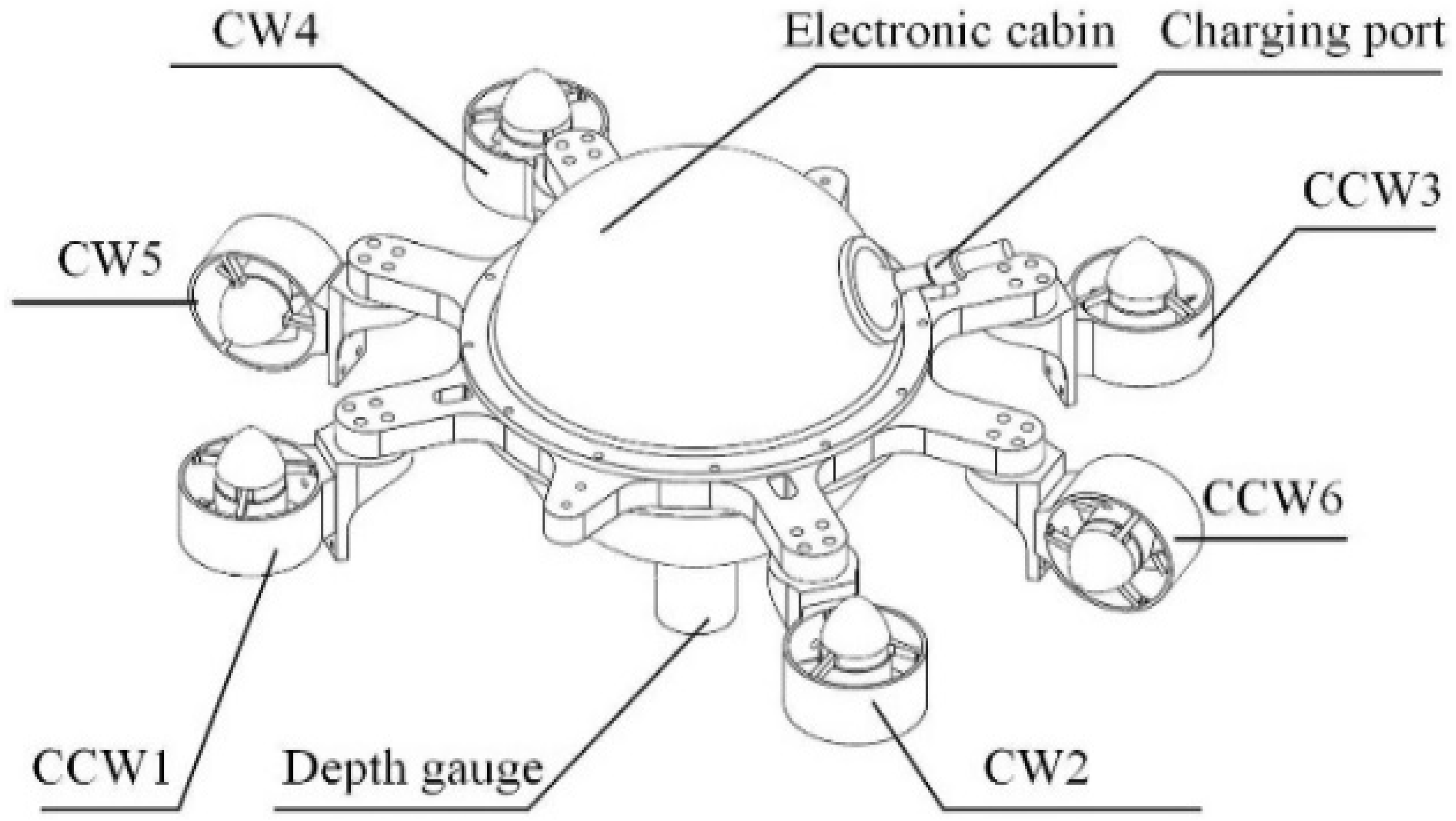
The structure of the S-ASUV described in this paper is shown in Figure 1, and comprises a spherical module and six propellers. The Hydrodynamic coefficients for each DOF is shown in

Table 1. Hydrodynamic coefficients for each DOF.

	Added Mass Coefficient	Linear Drag Coefficient	Nonlinear Drag Coefficient
surge	$X_{\dot{u}}$	$X_u$	${\overline{X}}_u$
sway	$Y_{\dot{v}}$	$Y_v$	${\overline{Y}}_v$
heave	$Z_{\dot{w}}$	$Z_w$	${\overline{Z}}_w$
roll	$K_{\dot{p}}$	$K_p$	${\overline{K}}_p$
pitch	$M_{\dot{q}}$	$M_q$	${\overline{M}}_q$
yaw	$N_{\dot{r}}$	$N_r$	${\overline{N}}_r$

.

Table 2. Main kinematic parameters.

	Force/Moment	Velocity	Position/Attitude
surge	X	u	x
sway	Y	v	y
heave	Z	w	z
roll	K	p	ϕ
pitch	M	q	θ
yaw	N	r	ψ

shows the S-ASUV’s force/moment, linear/angular velocity, and position/Euler angle for the six DOFs The main physical parameters of the S-ASUV are shown in

Table 3. Main parameters of S-ASUV.

Parameters	Symbol	Value
Mass	m (kg)	4.99
Gravity	G (N)	48.902
Buoyancy	B (N)	50.406
Sphere radius	γ (m)	0.0975
Length	l (m)	0.211
Center of gravity	(xg, yg, zg) (mm)	(0, 0, 11.15)
Moment of inertia	(Ix, Iy, Iz) (kg m2)	[0.01426, 0.01426, 0.01426]

, where m and γ are the mass and radius, respectively, l is the distance between the rotation axis and the propellers, B is the buoyancy, G is the force of gravity, (x_g, y_g, z_g) is the coordinates of the center of gravity, and (I_x, I_y, I_z) is the moment of inertia.

2.1. Frames of Reference

Dynamic models of AUVs are widely recognized for their non-linear, strongly coupled, time-varying nature and Multiple Input Multiple Output (MIMO) system attributes. These models encompass various hydrodynamic loads that are rarely constant over time. These loads are contingent on factors like speed, acceleration, and the size of the S-ASUV represented through hydrodynamic coefficients. These coefficients, detailed in Table 1, comprise the added mass and drag coefficients, delineating the vehicle’s dynamic behavior during acceleration and uniform motion, respectively [15].

Table 2 shows the S-ASUV’s force/moment, linear/angular velocity, and position/Euler angle for the six DOFs.

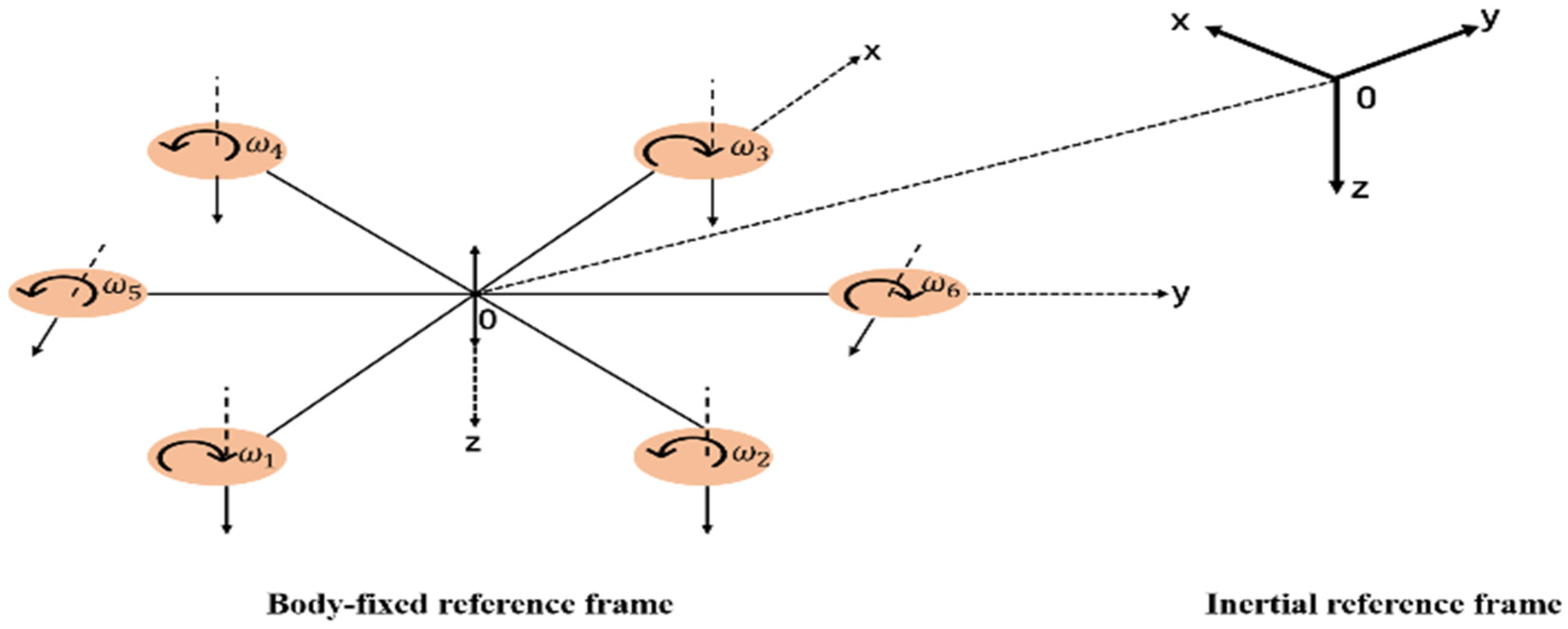
To facilitate mathematical analysis, we established two frames of reference. The body reference frame (BRF) is attached to the vehicle and aligned with its center of gravity (CG) as shown in Figure 2. Using this configuration, we could analyze the vehicle’s movement regarding the BRF relative to an inertial reference frame (IRF) that tracks the vehicle’s position and orientation globally. The thrusters are arranged in a cross shape, where the first and third propellers move clockwise with angular velocities of ω₁ and ω₃, generating downward thrust. In contrast, the second and fourth propellers make a counterclockwise motion with angular velocities of ω₂ and ω₄, generating downward thrust.

2.2. Kinematic and Dynamic Model

A complete kinematic and dynamic model of the S-ASUV can be seen in Section 2 of [15].

We introduced the subsequent vectors as defined below:

$${\eta }_1=\left[\begin{array}{c}x\\ y\\ z\end{array}\right],{\eta }_2=\left[\begin{array}{c}\varphi \\ \theta \\ \psi \end{array}\right],\eta =\left[\begin{array}{c}{\eta }_1\\ {\eta }_2\end{array}\right];$$

(1)

$$V_1=\left[\begin{array}{c}u\\ v\\ w\end{array}\right],V_2=\left[\begin{array}{c}p\\ q\\ r\end{array}\right],V=\left[\begin{array}{c}{V}_1\\ V_2\end{array}\right],$$

(2)

where η is the vector of position ${\eta }_1$ and pose ${\eta }_2$, i.e., Euler angle, and V is the velocity vector.

The kinematics equations of the AUV can be expressed as:

$$\left[\begin{array}{c}\dot{{\eta }_1}\\ \dot{{\eta }_2}\end{array}\right]=\left[\begin{array}{cc}{R}_1\left({\eta }_2\right)& 0_{3x3}\\ 0_{3x3}& R_2\left({\eta }_2\right)\end{array}\right]\left[\begin{array}{c}{V}_1\\ V_2\end{array}\right]$$

(3)

in which the conversion equations of the linear velocity and angular velocity are given as follows, where s = sin, c = cos, and t = tan:

$$\dot{{\eta }_1}=R_1\left({\eta }_2\right)V_1;$$

(4)

$$R_1\left({\eta }_2\right)=\left[\begin{array}{ccc}c\psi c\theta & c\psi s\theta s\varphi -s\psi s\varphi & s\psi s\varphi +c\psi c\varphi s\theta \\ s\psi c\theta & c\psi c\theta +s\psi s\theta s\varphi & s\theta s\psi c\varphi -c\psi s\varphi \\ -s\theta & c\theta s\varphi & c\theta c\varphi \end{array}\right];$$

(5)

$$\dot{{\eta }_2}=R_2\left({\eta }_2\right)V_2;$$

(6)

$$R_2({\eta }_2)=\left[\begin{array}{ccc}1& s\varphi t\theta & c\varphi t\theta \\ 0& c\varphi & -s\varphi \\ 0& s\varphi /c\theta & c\varphi /c\theta \end{array}\right].$$

(7)

Table 3 outlines the main parameters of the S-ASUV model used in the study. These parameters include mass (m), gravitational force (G), buoyancy force (B), radius (γ), length (l), center of gravity coordinates $x_g,y_g,z_g$ and moments of inertia about the principal axes $I_x,I_y,I_z$. These values serve as the foundational inputs for the simulation and analysis of the vehicle’s dynamic positioning performance.

2.3. Modeling of Dynamic Positioning Problem

The objective of this paper is to develop and implement a robust LBMPC algorithm for achieving precise DP of the multi-rotor dynamics of an S-ASUV in varying environmental conditions. The goal is to design a control system that ensures the S-ASUV maintains its desired position and orientation accurately and efficiently while mitigating the disturbances and uncertainties inherent in underwater operations using LMPC techniques.

We considered the motion of the vehicle in the local level plane. Two mild assumptions can be satisfied for the low-speed motion of the S-ASUV: (i) The vehicle has three planes of symmetry; and (ii) the mass distribution is homogeneous to simplify the mathematical model, reduce computational complexity, and focus on dominant horizontal motion. As a result, for motion control in the local level plane, the system matrices presented in [15] can be simplified. The inertia matrix becomes

$$M=\left[\begin{array}{cccccc}{M}_{\dot{u}}& 0& 0& 0& 0& 0\\ 0& M_{\dot{v}}& 0& 0& 0& 0\\ 0& 0& M_{\dot{w}}& 0& 0& 0\\ 0& 0& 0& M_{\dot{p}}& 0& 0\\ 0& 0& 0& 0& M_{\dot{q}}& 0\\ 0& 0& 0& 0& 0& M_{\dot{r}}\end{array}\right],$$

(8)

where $M_{\dot{u}}=m-X_{\dot{u}},M_{\dot{v}}=m-Y_{\dot{v}},M_{\dot{w}}=m-Z_{\dot{w}},M_{\dot{p}}=I_x-K_{\dot{p}},M_{\dot{q}}=I_y-M_{\dot{q}}\mathrm{and}{M}_{\dot{r}}=I_z-N_{\dot{r}}$ are the inertia terms including added mass. The restoring force is neglected, $g\left(\eta \right)=0$, and the damping matrix is

$$D\left(V\right)=\left[\begin{array}{cccccc}{X}_u+{\overline{X}}_u\left|u\right|& 0& 0& 0& 0& 0\\ 0& Y_v+{\overline{Y}}_v\left|v\right|& 0& 0& 0& 0\\ 0& 0& Z_w+{\overline{Z}}_w\left|w\right|& 0& 0& 0\\ 0& 0& 0& K_p+{\overline{K}}_p\left|p\right|& 0& 0\\ 0& 0& 0& 0& M_q+{\overline{M}}_q\left|q\right|& 0\\ 0& 0& 0& 0& 0& N_r+{\overline{N}}_r\left|r\right|\end{array}\right],$$

(9)

where $X_u,Y_v,Z_w,K_p,M_q\mathrm{and}{N}_r$ are the linear drag coefficients and ${\overline{X}}_u,{\overline{Y}}_v,{\overline{Z}}_w,{\overline{K}}_p,{\overline{M}}_q\mathrm{and}{\overline{N}}_r$ are the nonlinear drag coefficients. The Coriolis and centripetal matrix becomes:

$$C\left(V\right)=\left[\begin{array}{cccccc}0& 0& 0& 0& {-M}_{\dot{w}}w& M_{\dot{v}}v\\ 0& 0& 0& M_{\dot{w}}w& 0& -M_{\dot{u}}u\\ 0& 0& 0& {-M}_{\dot{v}}v& M_{\dot{u}}u& 0\\ 0& {-M}_{\dot{w}}w& M_{\dot{v}}v& 0& 0& -(M_{\dot{w}}{w}^2-M_{\dot{v}}{v}^2)\\ M_{\dot{w}}w& 0& -M_{\dot{u}}u& 0& 0& (M_{\dot{u}}{u}^2-M_{\dot{w}}{w}^2)\\ {-M}_{\dot{v}}v& M_{\dot{u}}u& 0& -(M_{\dot{w}}{w}^2-M_{\dot{v}}{v}^2)& (M_{\dot{w}}{w}^2-M_{\dot{u}}{u}^2)& 0\end{array}\right].$$

(10)

In the local level plane, the velocity vector $V={\left[u,v,w,p,q,r\right]}^T$ encloses the surge, sway, and yaw velocities, and the position and orientation vector $\eta ={\left[x,y,z,\varphi ,\theta ,\psi \right]}^T$ includes the position and heading of the vehicle.

By introducing disturbances and uncertainties, the dynamic model of the S-ASUV can be formulated as:

$$M\dot{V}+C\left(V\right)V+D\left(V\right)V+g\left(\eta \right)=\tau +{\tau }_E+{\mathsf{\Delta }\tau }_H,$$

(11)

where $\tau ={\left[A_u,A_v,A_w,A_p,A_q,A_r\right]}^T$ denotes the generalized thrust forces and moments. ${\tau }_E$ denotes the disturbance force/torque of the water flow environment and ${\mathsf{\Delta }\tau }_H$ denotes uncertain hydrodynamic forces/moments. The assumption is that the six propellers, denoted $u={\left[u_1,u_2,u_3,u_4,u_5,u_6\right]}^T$ within the local horizontal plane, collectively generate the generalized thrust force. It is important to note that these propellers were intentionally designed to remain fixed for simplicity, resulting in the representation of thrust allocation $\tau$ $=Su$ in which $S$ represents the thrust allocation matrix.

The kinematic Equation (3) can also be simplified as follows:

$$\dot{\eta }=K\left({\eta }_2\right)V,$$

(12)

where $K\left({\eta }_2\right)=\left[\begin{array}{cccccc}c\psi c\theta & -s\psi c\theta +c\psi s\theta s\varphi & s\psi s\varphi +c\psi s\theta c\varphi & 0& 0& 0\\ s\psi c\theta & c\psi c\theta +s\psi s\theta s\varphi & -c\psi s\varphi +s\psi s\theta c\varphi & 0& 0& 0\\ -s\theta & c\theta s\varphi & c\theta c\varphi & 0& 0& 0\\ 0& 0& 0& 1& 0& 0\\ 0& 0& 0& 0& 1& 0\\ 0& 0& 0& 0& 0& 1\end{array}\right]$.

We defined the system state as $\lambda ={\left[{\eta }^T,V^T\right]}^T$ and the generalized control input as $\tau$. The generalized control input $\tau$ is the resulting force of the thrusters. For S-ASUV, the experimental platform, six thrusters are effective in the local level plane. From (3) and (11), the dynamic model of the 3D DP problem with position and pose control is established below:

$$\dot{\lambda }=\left[\begin{array}{c}K\left({\eta }_2\right)V\\ M^{-1}(Su-C\left(V\right)V-D\left(V\right)V-g(\eta )\end{array}\right]=f(\lambda ,u),$$

(13)

where the state vector $\lambda ={\left[x,y,z,\varphi ,\theta ,\psi ,u,v,w,p,q,r\right]}^T$. The DP model in (13) of S-ASUV reveals the dynamics from the thrusters to the position and pose in 3D space, facilitating 3D DP control using LBMPC. The hydrodynamic coefficients for the S-ASUV in (13) are summarized in

Table 4. Hydrodynamic coefficient summary.

Inertia Term	Linear Drag	Nonlinear Drag
$M_{\dot{u}}=3.0003\mathrm{k}\mathrm{g}$	$X_u=-0.7318\mathrm{k}\mathrm{g}/\mathrm{s}$	${\overline{X}}_u=3.006\mathrm{k}\mathrm{g}/\mathrm{m}$
$M_{\dot{v}}=3.0003\mathrm{k}\mathrm{g}$	$Y_v=-0.7318\mathrm{k}\mathrm{g}/\mathrm{s}$	${\overline{Y}}_v=3.006\mathrm{k}\mathrm{g}/\mathrm{m}$
$M_{\dot{w}}=1.8563\mathrm{k}\mathrm{g}$	$Z_w=0.3747\mathrm{k}\mathrm{g}/\mathrm{s}$	${\overline{Z}}_w=36.35\mathrm{k}\mathrm{g}/\mathrm{m}$
$M_{\dot{p}}=0.087\mathrm{k}\mathrm{g}{\mathrm{m}}^2$	$K_p=0.001359\mathrm{k}\mathrm{g}{\mathrm{m}}^2/\mathrm{s}$	${\overline{K}}_p=0.000012\mathrm{k}\mathrm{g}{\mathrm{m}}^2$
$M_{\dot{q}}=0.087\mathrm{k}\mathrm{g}{\mathrm{m}}^2$	$M_q=0.001359\mathrm{k}\mathrm{g}{\mathrm{m}}^2/\mathrm{s}$	${\overline{M}}_q=0.000012\mathrm{k}\mathrm{g}{\mathrm{m}}^2$
$M_{\dot{r}}=01553\mathrm{k}\mathrm{g}{\mathrm{m}}^2$	$N_r=0.006736\mathrm{k}\mathrm{g}{\mathrm{m}}^2/\mathrm{s}$	${\overline{N}}_r=0.008206\mathrm{k}\mathrm{g}{\mathrm{m}}^2$

.

For model (13), the following essential properties can be easily explored and will be exploited in the controller design:

• P-1: The inertia matrix is positive definite and upper bounded: 0 < M = M^T ≤ $\overline{m}I$ < ∞.
• P-2: The Coriolis and centripetal matrix is skew-symmetric: C(V) = −C^T(V).
• P-3: The inverse of rotation matrix satisfies $K^{-1}\left(\psi \right)=K^T\left(\psi \right)$, and preserves length $\parallel K^T\left(\psi \right)\dot{\eta }{\parallel }_2=\parallel {\dot{\eta }\parallel }_2$.
• P-4: The damping matrix is positive definite: D(V) > 0.
• P-5: The input matrix satisfies that SS^T is nonsingular.
• P-6: The restoring force g(η) is bounded: $\parallel {g\left(\eta \right)\parallel }_{\infty }\le \overline{g}$.
• While we initially assumed $g\left(\eta \right)=0$ in Section 2.2 for simplicity, we recognize and acknowledge in subsequent sections (P-6 and Assumption 2) that $g\left(\eta \right)$ exists within defined bounds. This acknowledgment ensures that our model accounts for the bounded and modest influence of the restoring force, aligning with physical constraints and operational scenarios.

This research focuses on achieving precise three-dimensional dynamic positioning for the S-ASUV while maintaining robustness in complex underwater environments. To this end, this work integrated multivariable PID into the LMPC scheme with Lyapunov stability analysis, enhancing control performance and stability. The study conducted rigorous feasibility and stability analyses, ensuring robustness to external disturbances and model uncertainties.

2.4. Formulation of Optimization Problem

DP control refers to the implementation of feedback control techniques in S-ASUV, and the goal is to maintain a desired position and orientation through the adjustment of propeller thrust alone. Numerous existing DP controllers have been devised using the Lyapunov direct method, boosting global stability attributes. Explicitly incorporating these controllers allows us to formulate the LMPC problem for DP control [16]. Considering the preferred location and orientation indicated by ${\eta }_d={\left[x_d,y_d,z_d,{\varphi }_d,{\theta }_d,{\psi }_d\right]}^T$, the nonlinear optimization problem ($P_0$) of DP for S-ASUV can be formulated as:

$$\underset{\widehat{u}\in G\left(\mu \right)}{\min }J=\underset{0}{\overset{T}{\int }}\left(\parallel \tilde{\lambda }\left(s\right){\parallel }_X^2+\parallel \widehat{u}\left(s\right){\parallel }_Y^2\right)ds+\parallel \tilde{\lambda }\left(T\right){\parallel }_Z^2;$$

(14)

Subject to

$$\dot{\lambda }\left(s\right)=f\left(\widehat{\lambda }\left(s\right),\widehat{u}\left(s\right)\right),$$

(15)

$$\widehat{\lambda }\left(0\right)=\lambda \left(t_0\right),$$

(16)

$$\left|\widehat{u}\left(s\right)\right|\le u_{max},$$

(17)

$${\displaystyle \frac{\mathsf{\partial }W}{\mathsf{\partial }\lambda }}f(\widehat{\lambda }\left(0\right),\widehat{u}\left(0\right))\le {\displaystyle \frac{\mathsf{\partial }W}{\mathsf{\partial }\lambda }}f(\widehat{\lambda }\left(0\right),\omega \left(\widehat{\lambda }\left(0\right)\right)),$$

(18)

where $\widehat{\lambda }\left(s\right)$ stands for the planned trajectory of the AUV’s state, using the system’s model to evolve; $\tilde{\lambda }=\mathrm{c}\mathrm{o}\mathrm{l}\left(\widetilde{\eta ,}\widehat{V}\right)$ represents the error state where $\tilde{\eta }=\widehat{\eta }-{\eta }_d$; $G\left(\mu \right)$ represents a collection of piece-wise constant functions based on the sampling period $\mu$. $T=N\mu$ indicates the forecasting horizon, X, Y, and Z represent the weighting matrices and are guaranteed to maintain positive definiteness. It is noted that $\omega$ (·) conventionally denotes the PD controller, while herein, for LBMPC, we propose the PID secondary controller, which is demonstrated in Section 3.2. At the same time, W (·) signifies the corresponding Lyapunov function.

2.5. PID Secondary Control Law

Unlike modern LMPC techniques [15,17], which employ a PD secondary control law, a multi-variable PID controller was used as the secondary law, enhancing the rapidity and accuracy of the DP control. For the theoretical explanation, the designed PID secondary law also introduced disturbance and model uncertainties, playing a role in resisting disturbances and uncertainties. The used multi-variable PID control law is:

$$\tau \left(\lambda \right)=g\left(\eta \right)-{\tau }_{\mathrm{E}}-{\mathsf{\Delta }\tau }_{\mathrm{H}}-K^T\left({\eta }_2\right){\tau }_{PID};$$

(19)

$${\tau }_{PID}=K_p\tilde{\eta }+K_d\dot{\eta }+K_i\mathsf{\Delta }\tilde{\eta },$$

(20)

where $\mathsf{\Delta }\tilde{\eta }={\int }_0^{t}K\left({\eta }_2\right)Vds$; then, one can easily obtain $\dot{\left(∆\tilde{\eta }\right)}=K\left({\eta }_2\right)V$. The user defines the control gain matrices $K_p\mathrm{and}{K}_d\mathrm{and}{K}_i$, which should be diagonal and positive definite. It is important to note that ${\tau }_{\mathrm{E}}\mathrm{a}\mathrm{n}\mathrm{d}{\mathsf{\Delta }\tau }_{\mathrm{H}}$ were not directly implemented in the control algorithm. Instead, they were adjusted through parameters in the digital experiments to represent real-life disturbances. This unconventional approach was adopted to evaluate the robustness and performance of the PID control law under various disturbance scenarios.

The proposed choice for the Lyapunov function is the following:

$$W={\displaystyle \frac{1}{2}}{V}^{T}MV+{\displaystyle \frac{1}{2}}{\tilde{\eta }}^T{K}_p\tilde{\eta }+{\displaystyle \frac{1}{2}}{(∆\tilde{\eta })}^T{K}_i∆\tilde{\eta }$$

(21)

When computing the time derivative of W along the trajectory of the closed-loop system, using the product rule and noting that $M,K_p\mathrm{and},K_i$ are constant matrices, we differentiated each term separately. Combining these results, we obtained:

$$\dot{W}=V^{T}M\dot{V}+{\dot{\eta }}^T{K}_p\tilde{\eta }+{\dot{\left(∆\tilde{\eta }\right)}}^T{K}_i∆\tilde{\eta };$$

(22)

Substituting (11), (12), (19), and (20) into (22) yields

$$\dot{W}=-V^T\left[C\left(V\right)+D\left(V\right)+K_d^{*}\left(\eta \right)\right]V,$$

(23)

where $K_d^{\mathrm{*}}=R^T\left({\eta }_2\right)K_{d}R\left({\eta }_2\right)$. Considering $V^{T}C\left(V\right)V=0$ for all V, we have

$$\dot{W}=-V^T\left[D\left(V\right)+K_d^{*}\left(\eta \right)\right]V\le 0$$

(24)

The gain parameter $K_d^{*}\left(\eta \right)>0$ is positive. Following [18], LaSalle’s theorem indicates that the closed-loop system, influenced by the nonlinear PID controller, would exhibit global asymptotic stability relative to the equilibrium point $\left[\tilde{\eta },V\right]=[0,0]$.

A comprehensive description of the contraction constraint (18) associated with the use of nonlinear PID control follows:

$$\begin{gathered} \widehat{V}{\left(0\right)}^T\left(\widehat{u}\left(O\right)-C\left(\widehat{V}\left(\mathsf{O}\right)\right)\widehat{V}\left(O\right)-D\left(\widehat{V}\left(O\right)\right)\widehat{V}\left(O\right)-g\left(\widehat{\eta }\left(O\right)\right)+ \\ {R}^T\left(\widehat{\psi }\left(O\right)\right)K_p\tilde{\eta }\left(O\right)\right)\le -\widehat{V}{\left(O\right)}^T[D\left(\widehat{V}\left(O\right)\right)+K_d^{*}\left(\widehat{\eta }\left(O\right)\right)]\widehat{V}\left(O\right). \end{gathered}$$

(25)

To ensure recursive feasibility, it is worth noting that the PID controller, $\omega \left(\widehat{\lambda }\right)$, remains viable for the LBMPC (14), (15), (16), (17), and (18) as long as we can satisfy the condition $\left|\omega \right(\widehat{\lambda }\left)\right|\le u_{max}$.

The following uses several logical and realistic assumptions to simplify calculations.

Assumption 1.

The maximum capacity of the propellers is the same, i.e., $\left|u_i\right|\le U_{max}$. Note that Assumption 1 is plausible and frequently accurate in real-world situations.

The proposition that follows is then;

Proposition 1.

Consider the Moore–Penrose pseudoinverse implementation when allocating thrust, that is,

$$u=S^T{\left(S{S}^T\right)}^{-1}\tau =S^{+}\tau$$

(26)

and signify the highest generalized thrust force possible by ${\tau }_{max}=\parallel {\tau }_{max}{\parallel }_{\mathrm{\infty }}$ with ${\tau }_{max}={\left[A_{u,max},A_{v,max},A_{w,max,}{A}_{p,max},A_{q,max},A_{r,max}\right]}^T$. If this relationship holds:

$${\tau }_{max}\le {\displaystyle \frac{u_{max}}{{\overline{j}}^{+}}}$$

(27)

where ${\overline{j}}^{+}=\parallel S^{+}{\parallel }_{\infty }$, then it is always possible to allocate the thrust, that is, $\parallel u{\parallel }_{\infty }\le u_{max}$.

Proof. 

If we take the infinity norm on either side of (26) we obtain

$$\parallel u{\parallel }_{\infty }={\parallel S}^{+}\tau {\parallel }_{\infty }\le {\overline{j}}^{+}\parallel \tau {\parallel }_{\infty }\le {\overline{j}}^{+}{\tau }_{max}.$$

(28)

Considering (27) and Assumption 1, (28) becomes

$$\parallel u{\parallel }_{\infty }\le {\overline{j}}^{+}{\tau }_{max}\le u_{max}.$$

(29)

□

Assumption 2.

The restoring force $g\left(\eta \right)$ is limited in magnitude and relatively modest, such that

$$\parallel g\left(\eta \right){\parallel }_{\infty }\le \overline{g}<{\tau }_{max},$$

(30)

where $\overline{g}$ denotes the input bound.

The second assumption is likewise a valid one. Sine and cosine function combinations are included in the comprehensive definition of $g\left(\eta \right)$. Therefore, we can ensure that the restoring force remains within certain bounds. Moreover, it is worth noting that the upper bound $\overline{g}$ is considerably smaller in magnitude compared to the maximum allowable thrust force ${\tau }_{max}$. Failing to meet this condition would render the feedback control infeasible, which is not considered in this study.

2.6. Stability Analysis

In this subsection, the feasibility and stability of the proposed LBMPC are both rigorously proved, guaranteeing the closed-loop stability of the DP control system.

Theorem 1.

Assume that the control gains $K_P,K_{d}and{K}_i$ are each equal to $diag\left\{k_{pi}\right\},diag\left\{k_{di}\right\}anddiag\left\{k_{ii}\right\}$. Let ${\overline{k}}_p=max\left\{k_{pi}\right\}$; ${\overline{k}}_d=max\left\{k_{di}\right\}$ and ${\overline{k}}_i=max\left\{k_{ii}\right\}$ represent the greatest elements in $K_p,K_{d}and{K}_i$, respectively, and suppose assumptions one and two can hold and define $\omega \left(\lambda \right)=S^{+}\tau \left(\lambda \right)$. If the relationship shown below can hold:

$$\left({\overline{k}}_p+\sqrt{2}{\overline{k}}_d+{\overline{k}}_i\right)\le {\displaystyle \frac{{\tau }_{max}-\overline{g}}{\sqrt{2}}},$$

(31)

where $\tilde{\lambda }\left(0\right)$ denotes the initial error and ${\tau }_{max}$ adheres to Equation (27), the LBMPC problem ($P_0$) recognizes recursive feasibility. In other words, $\left|\omega \left(\widehat{\lambda }\left(t\right)\right)\right|\le u_{max}forallt\ge 0where{u}_{max}=u_{max}1$.

Proof of Theorem 1.

By applying the infinity norm to both sides of Equation (19), we obtain:

$$\begin{gathered} \parallel \tau {\parallel }_{\infty }=\parallel g\left(\eta \right)-{\mathsf{\tau }}_{\mathrm{E}}-{\mathsf{\Delta }\mathsf{\tau }}_{\mathrm{H}}-R^T\left(\psi \right){\tau }_{PID}{\parallel }_{\infty }\le \parallel g\left(\eta \right){\parallel }_{\infty }+\parallel R^T\left(\psi \right){\parallel }_{\infty }\parallel {\tau }_{PID}{\parallel }_{\infty }\le \\ \overline{g}+\sqrt{2}\parallel {\tau }_{PID}{\parallel }_{\infty }. \end{gathered}$$

(32)

Since $\parallel R^T\left(\psi \right){\parallel }_{\mathrm{\infty }}=\max \left\{cos\psi -sin\psi ,sin\psi +cos\psi ,1\right\}\le \sqrt{2}$.

From (12) and (20), we have

$$\begin{gathered} \parallel {\tau }_{PID}{\parallel }_{\infty }=\parallel K_p\tilde{\eta }+K_d\dot{\eta }+K_i∆\tilde{\eta }{\parallel }_{\infty }=\parallel K_p\tilde{\eta }+K_{d}R\left(\psi \right)V+K_i∆\tilde{\eta }{\parallel }_{\infty }\le {\overline{k}}_p\parallel \tilde{\eta }{\parallel }_{\infty }+ \\ \sqrt{2}{\overline{k}}_d\parallel V{\parallel }_{\infty }+{\overline{k}}_i\parallel {\tilde{\eta }}_2{\parallel }_{\infty }\le ({\overline{k}}_p+\sqrt{2}{\overline{k}}_d+{\overline{k}}_i)\parallel \tilde{\lambda }{\parallel }_{\infty }. \end{gathered}$$

(33)

As (18) is fulfilled, it allows for $\dot{V}\le 0$. Consequently, we can conclude that $\parallel \tilde{\lambda }{\parallel }_2\le \parallel \tilde{\lambda }\left(0\right){\parallel }_2$. Considering $\parallel \tilde{\lambda }{\parallel }_{\infty }\le$ $\parallel \tilde{\lambda }{\parallel }_2$, we arrive at:

$$\parallel {\tau }_{PID}{\parallel }_{\infty }\le \left({\overline{k}}_p+\sqrt{2}{\overline{k}}_d+{\overline{k}}_i\right)\parallel \tilde{\lambda }\left(0\right){\parallel }_2.$$

(34)

Together with (32), we have

$$\parallel \tau {\parallel }_{\infty }\le \overline{g}+\sqrt{2}({\overline{k}}_p+\sqrt{2}{\overline{k}}_d+{\overline{k}}_i)\parallel \tilde{\lambda }\left(\mathsf{O}\right){\parallel }_2.$$

(35)

If we can meet condition (31), then the subsequent relationship is valid.

$$\parallel \tau {\parallel }_{\infty }\le \overline{g}+\sqrt{2}\left({\overline{k}}_p+\sqrt{2}{\overline{k}}_d+{\overline{k}}_i\right)\parallel \tilde{\lambda }\left(0\right){\parallel }_2.\le {\tau }_{max}.$$

(36)

With (27), we can guarantee that $\parallel \omega \left(\widehat{\lambda }\left(t\right)\right){\parallel }_{\infty }\le u_{max}$ remains consistently satisfied, thereby concluding the proof.

We observe that it is straightforward to fulfill condition (31) by assigning ${\overline{k}}_p,{\overline{k}}_d\mathrm{and}{\overline{k}}_i$ arbitrarily small positive values. The size of the region of attraction can be flexible as the assurance of closed-loop stability is provided through recursive feasibility. □

Theorem 2.

Suppose that both Assumptions 1 and 2 are met. In that case, the LBMPC dynamic positioning control will ensure the continuous stability of the required equilibrium point $\left[\tilde{\eta },V\right]=[0,0]$. Additionally, by employing sufficiently small control gains ${\overline{k}}_p,{\overline{k}}_{d}and{\overline{k}}_i$, the region of attraction can be significantly expanded.

Proof of Theorem 2.

The proof first shows that the equilibrium is asymptotically stable and then demonstrates that one can adjust the size of the region where the system’s trajectories will converge to equilibrium as needed. Applying the reverse Lyapunov theorem [15], given that we have already identified a continuously differentiable and unbounded Lyapunov function $W\left(\lambda \right)$ in (21), continuously differentiable and radically unbounded by converse Lyapunov theorems (31), there exist functions such as ${\beta }_i\left(·\right),i=1,2,3$ belonging to the class ${\chi }_{\infty }$ that satisfy the subsequent inequalities:

$${\beta }_1\left(\parallel \lambda \parallel \right)\le W\left(\lambda \right)\le {\beta }_2\left(\parallel \lambda \parallel \right);$$

(37)

$${\displaystyle \frac{\mathsf{\partial }W}{\mathsf{\partial }\lambda }}b\left(\lambda ,h\left(\lambda \right)\right)\le {-\beta }_3\left(\parallel \lambda \parallel \right).$$

(38)

Considering (18) and the fact that each sampling period will only use the first component of $\chi \left(\lambda \right)$, we obtain

$${\displaystyle \frac{\mathsf{\partial }W}{\mathsf{\partial }\lambda }}b\left(\lambda ,u\left(\lambda \right)\right)\le {\displaystyle \frac{\mathsf{\partial }W}{\mathsf{\partial }\lambda }}b\left(\lambda ,h\left(\lambda \right)\right)\le {-\beta }_3\left(\parallel \lambda \parallel \right).$$

(39)

We affirm that employing common Lyapunov arguments, the closed-loop system under LBMPC $u\left(\lambda \right)$ is asymptotically stable and possesses a region of attraction using common Lyapunov arguments (such as Theorem 4.8 in [15]).

$$\kappa =\{\lambda \in {\mathbb{R}}^n|({\overline{k}}_p+\sqrt{2}{\overline{k}}_d+{\overline{k}}_i)\parallel \tilde{\lambda }{\parallel }_2\le {\displaystyle \frac{{\tau }_{max}-\overline{g}}{\sqrt{2}}}\},$$

(40)

where $\tilde{\lambda }=col(\tilde{\eta },V)$ represents the error state.

We chose the control gains $K_p>0,K_d>0\mathrm{and}{K}_i>0$ meeting the arbitrary big initial error condition $\tilde{\lambda }$, therefore satisfying

$$({\overline{k}}_p+\sqrt{2}{\overline{k}}_d+{\overline{k}}_i)\le {\displaystyle \frac{{\tau }_{max}-\overline{g}}{\sqrt{2}\parallel \tilde{\lambda }{\parallel }_2}}.$$

(41)

Therefore, the closed-loop system exhibits stability, affirming the solvability of the LBMPC problem. The extent of the region of attraction can be adjusted as needed as long as there are sufficient small control gains to satisfy (41) because there are no other restrictions on ${\overline{k}}_p,{\overline{k}}_d\mathrm{and}{\overline{k}}_i$. □

Remark 1.

The magnitude of the control gains impacts the PID controller’s control performance, despite the fact that asymptotic stability relies solely on the control gain matrices $K_p,K_{d}and{K}_i$ being positively definite. A slower rate of convergence would result from smaller control gains. Nevertheless, although significantly small control gains were chosen to attain a broad region of attraction in the proposed LBMPC DP control, the optimization procedure allows the system to effectively leverage its thrust capability to achieve optimal control performance consistent with the objective function (14).

2.7. LBMPC DP Control Algorithm

MPC leverages a dynamic model of the controlled system to predict future states over a finite time horizon. By solving an optimization problem, it minimizes future control errors while adhering to system constraints, thereby ensuring optimal control performance.

The LBMPC DP control algorithm can be followed by a list of steps that describe how the algorithm will be executed, below:

(i)

At the current sampling instant t₀, considering the system’s present state $\lambda \left(t_0\right)$, we address the optimal control problem (P₀); let $\xi \left(s\right)$ represent the sub-optimal solution;

(ii)

the S-ASUV applies $\xi \left(s\right)$ for just a single sampling interval: $u\left(t\right)=\xi \left(s\right)\mathrm{for}s\in [0,\mu ]$;

(iii)

At the subsequent sampling instant $t_0+\mu$, a fresh measurement of the system’s state $\lambda (t_0+\mu )$ is incorporated as feedback; then, (P₀) is solved once more, starting anew with the fresh initial condition $\lambda (t_0+\mu )$. The process iterates, recommencing from step (i).

3. Results

In this section, the primary purpose lies in validating and verifying the performance of the proposed method, ensuring accuracy and effectiveness. The dynamic model of the S-ASUV, established using the data in [15], is employed in this part. To test the advantages of the proposed method, the classical PD [19] and modern controllers including MPC [20] and LMPC [14] were used in a series of experiments for comprehensive comparison.

3.1. Selection of Parameters

We set the target position, represented by ${\eta }_d={\left[0,0,0,0,0,0\right]}^T$, to be situated at the origin of the IRF, and this decision was made to maintain simplicity without compromising generality. According to experimental data in [21], the actual maximum force output for each propeller is 8N. In order to tackle the LBMPC problem formulated in Equations (14)–(18), we utilized a discretization strategy coupled with Sequential Quadratic Programming (SQP) to obtain a solution. This can be followed by a list of the variables that were chosen.

Sampling period $\mu =0.02\left[\mathrm{s}\right]$,

Prediction horizon $T=5\mu$,

Weighting matrices:

• $X=diag\left({10}^4,{10}^4,{10}^3,{10}^2,{10}^2,{10}^2,{10}^{-2},{10}^{-2},{10}^{-2},{10}^{-2},{10}^{-2},{10}^{-2}\right)$,
• $Y=diag({10}^{-2},{10}^{-2},10^{-2},{10}^{-2},{10}^{-2}{,10}^{-2},{10}^3,{10}^2,{10}^2,10,10,10)$,
• $Z=diag(10,10,10,10,10,10,10,10,10,10,10,10)$,

Control gains for nonlinear PID control: $K_p=K_d=K_i=diag(8,8,8,8,8,8)$,

Starting state: $\lambda \left(0\right)={\left[5,5,-{\displaystyle \frac{\pi }{2}},0,0,0,0,0,0,0,0,0\right]}^T$,

• $U_{max}=8$ for each propeller,
• $U_{min}=-8$ for each propeller,

The thrust allocation matrix

$$S=\left|\begin{array}{cccccc}0.07974& 008643& 0.08127& 0.08270& 0& 0\\ 0.06032& 0.05029& -0.05824& -0.05610& 0& 0\\ 0.02945& -0.03302& -0.02847& 0.03505& 0& 0\\ 0& 0& 0& 0& 0.02945& -0.03302\\ 0& 0& 0& 0& -0.03302& -0.02847\\ 0& 0& 0& 0& -0.02847& 0.03505\end{array}\right|.$$

(42)

3.2. Performance Comparison and Analysis

3.2.1. Performance Without Disturbances and Uncertainties

In our study, we utilized MATLAB R2022b, a widely recognized programming environment provided by MathWorks, for implementing and testing our algorithms. The simulations were conducted using a custom MATLAB script, allowing for precise control over algorithm development and execution.

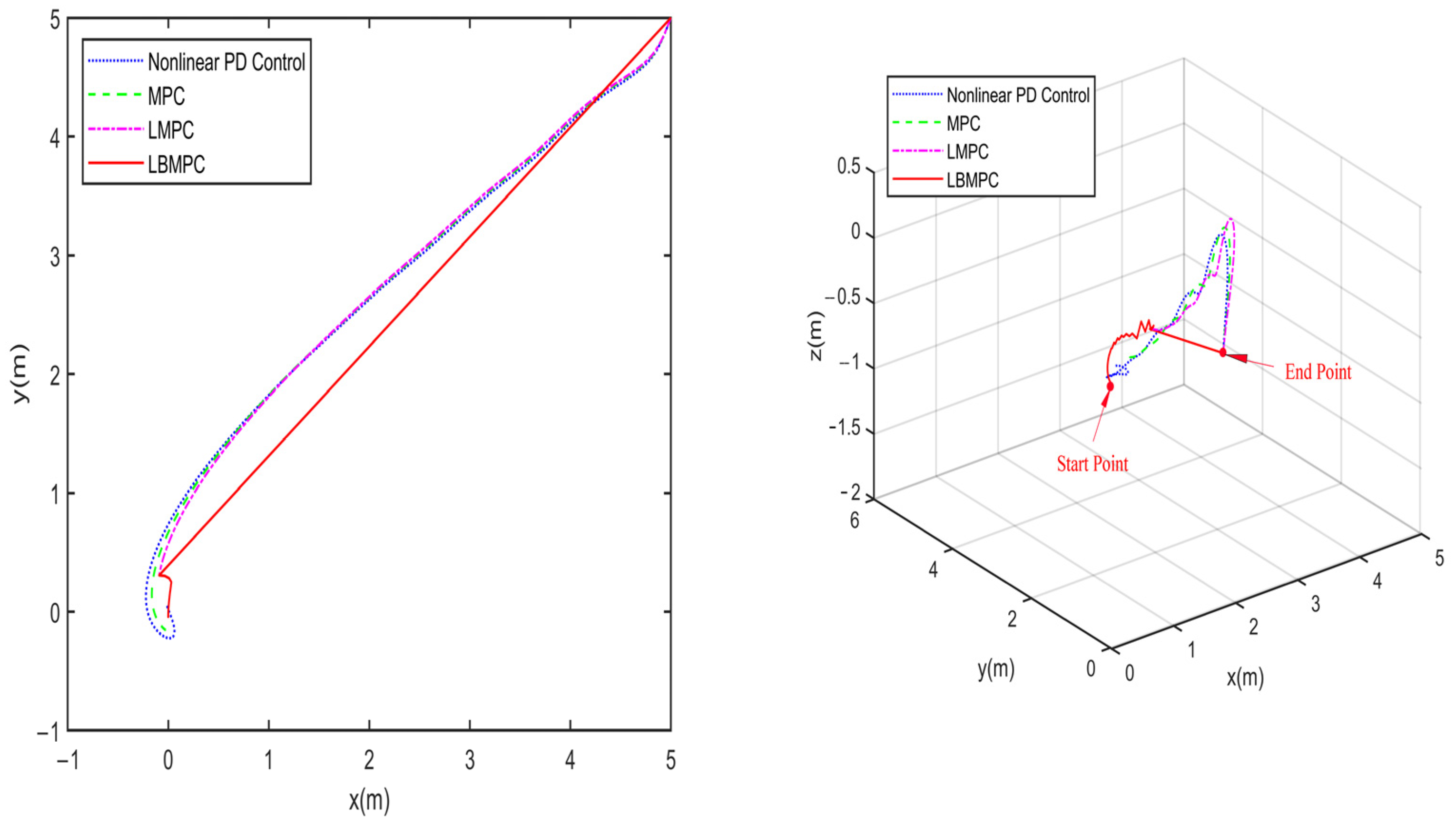
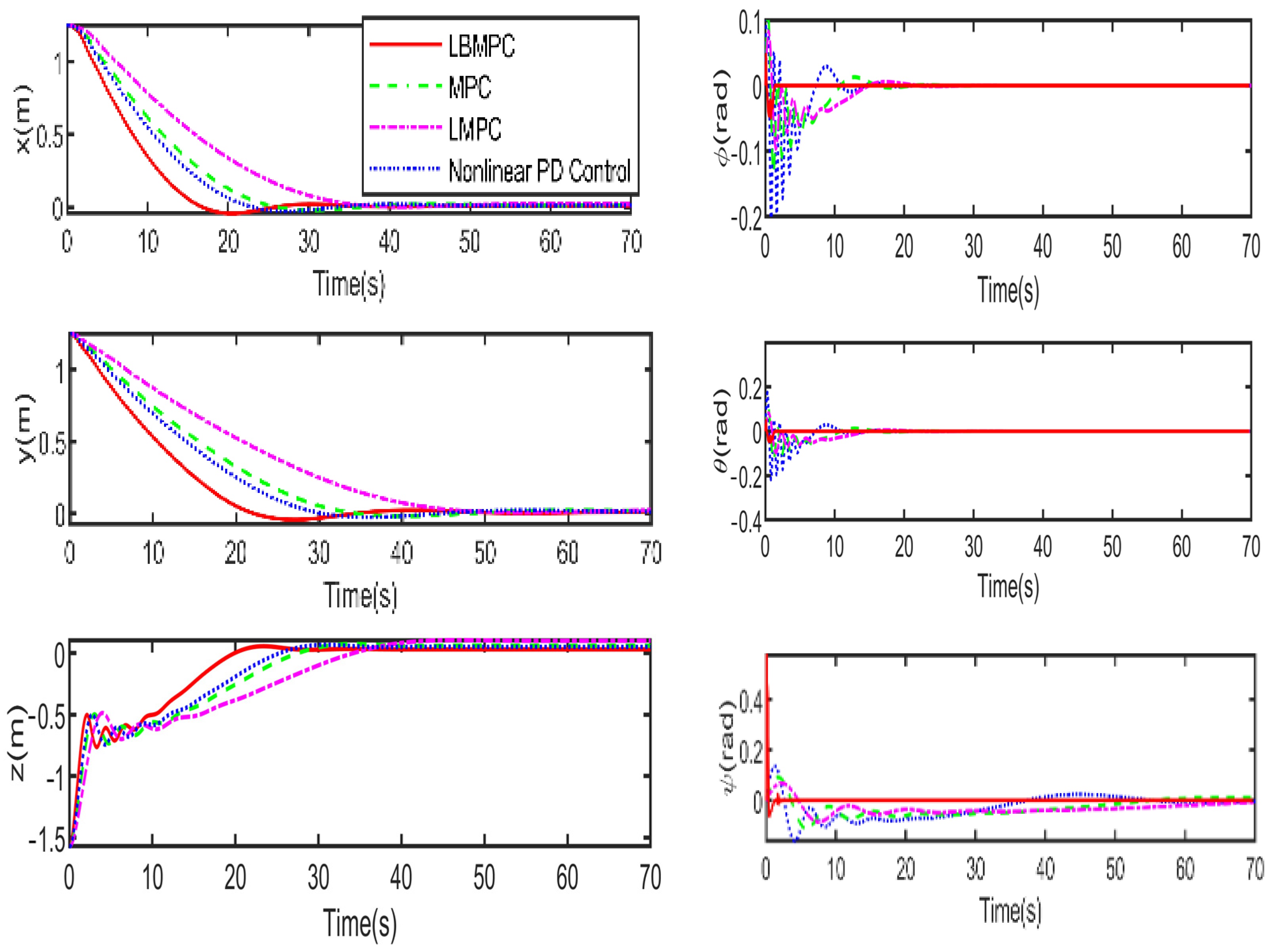
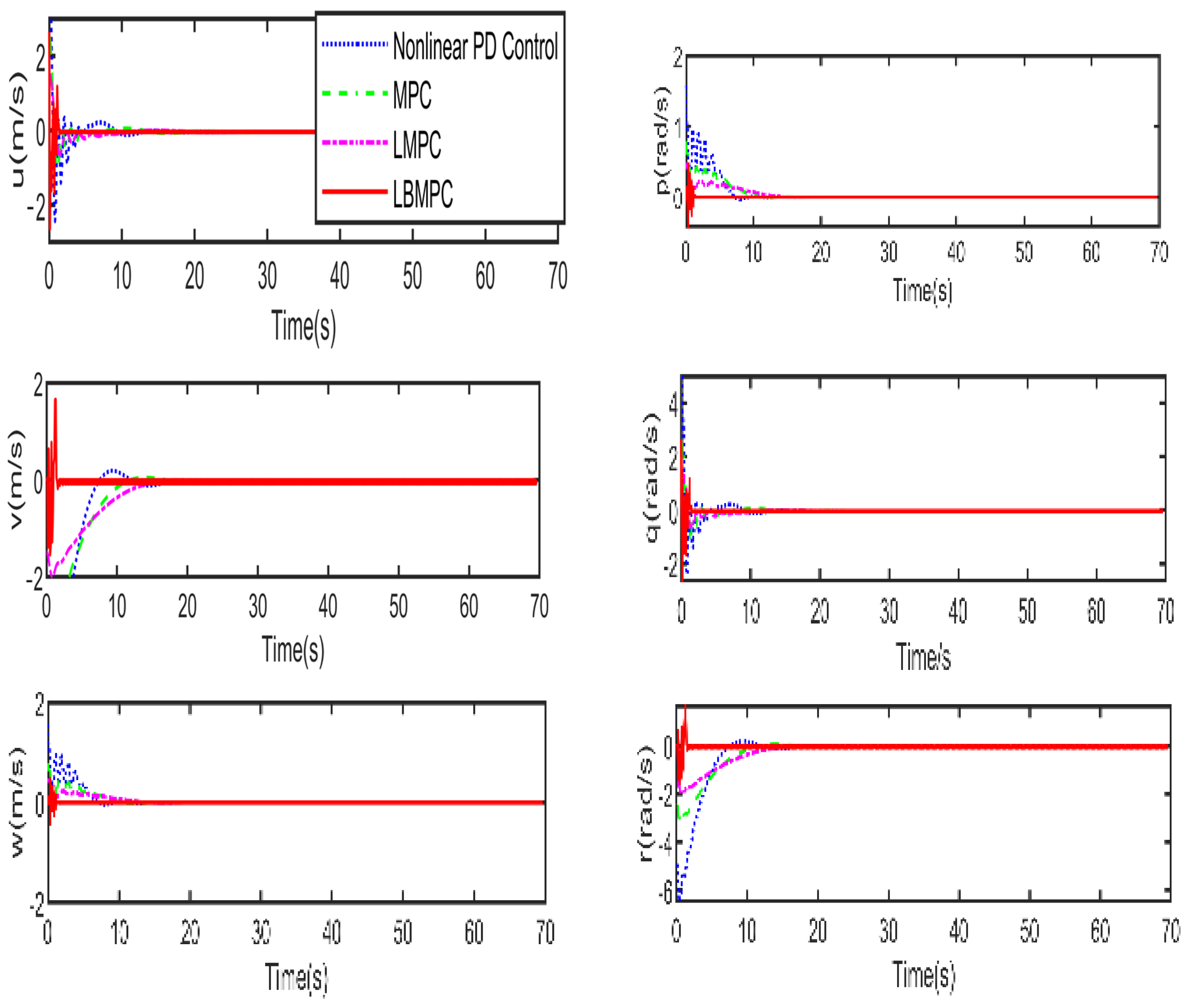
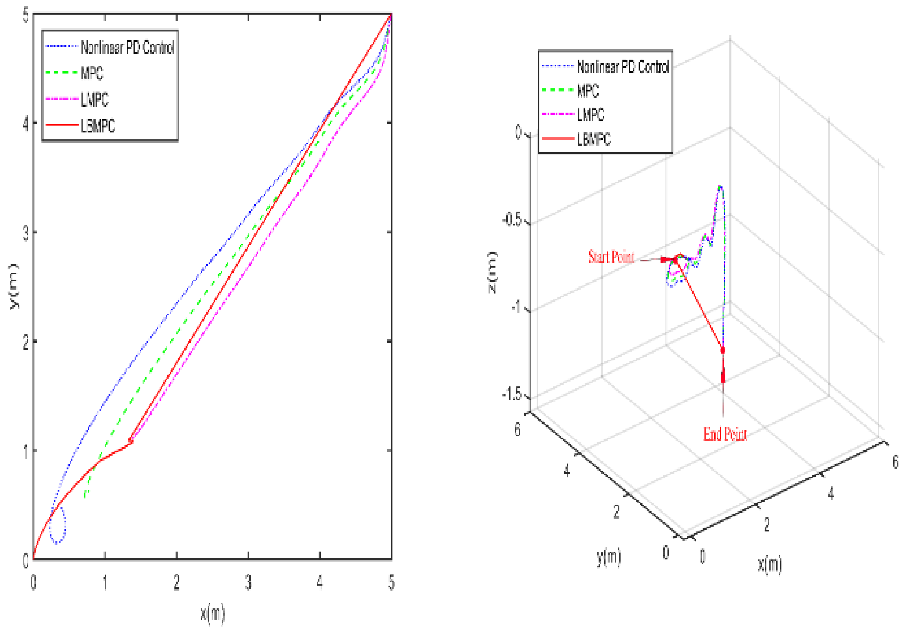
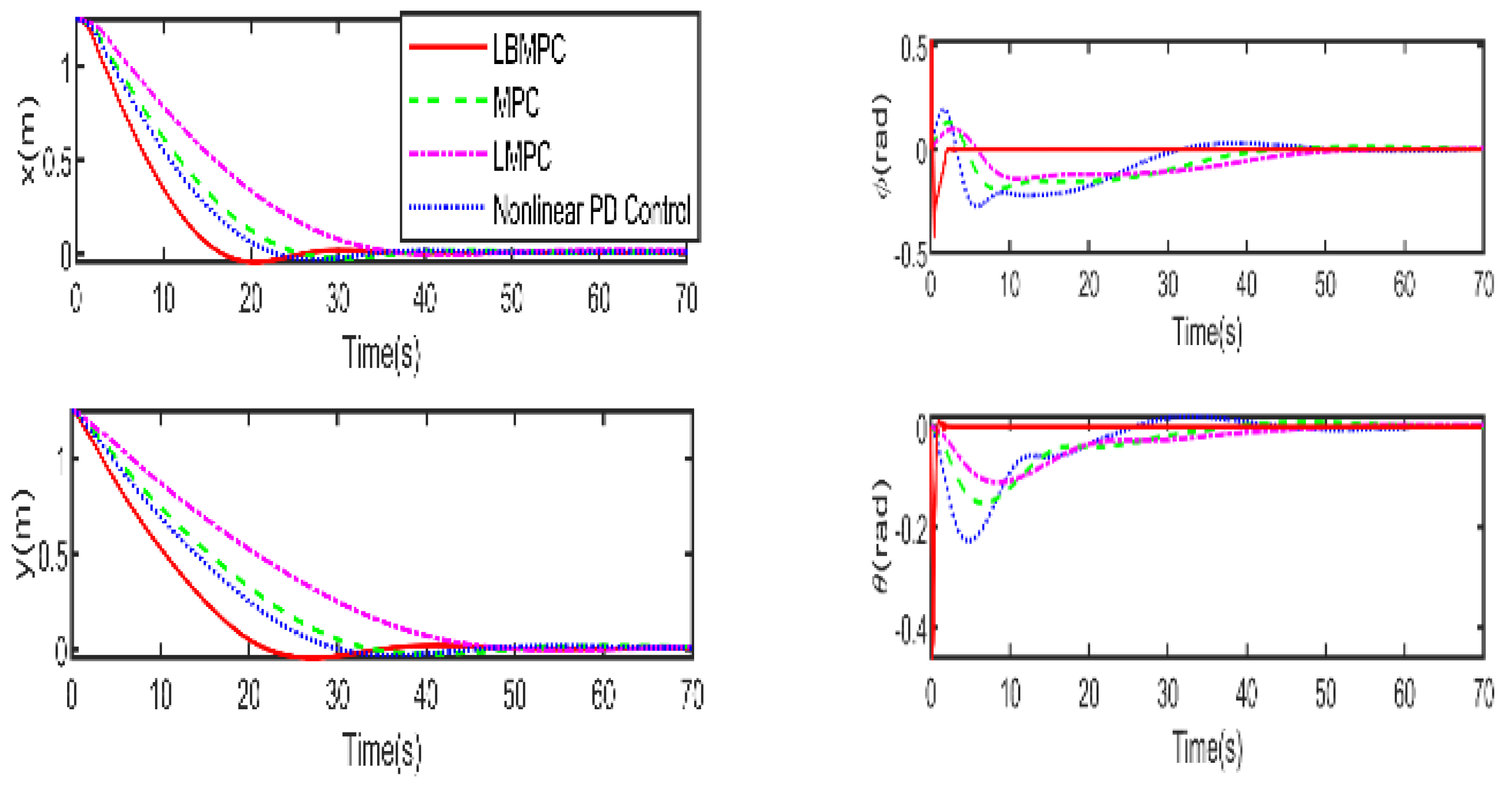
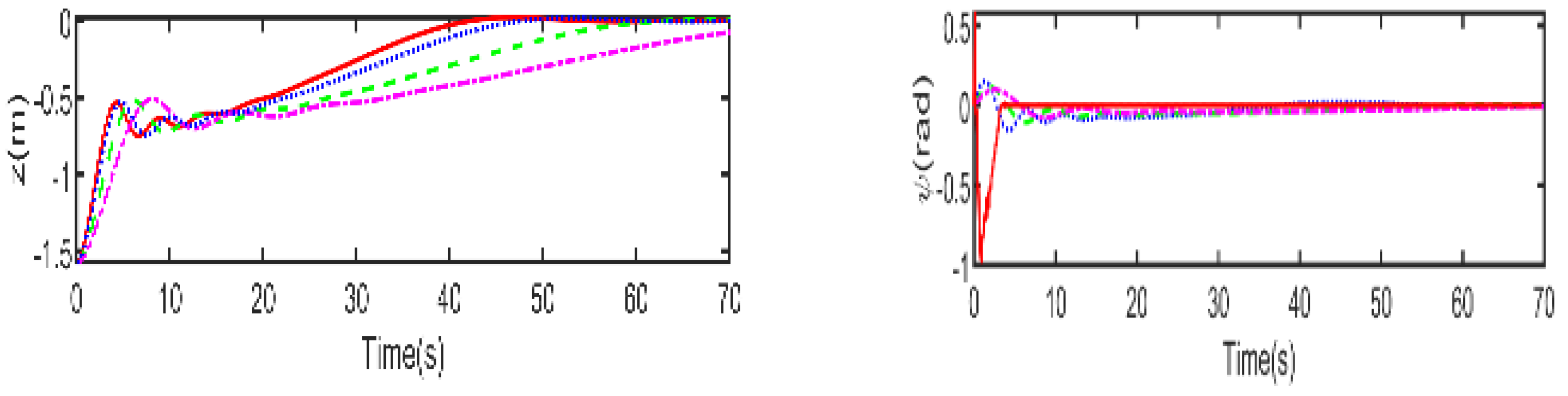
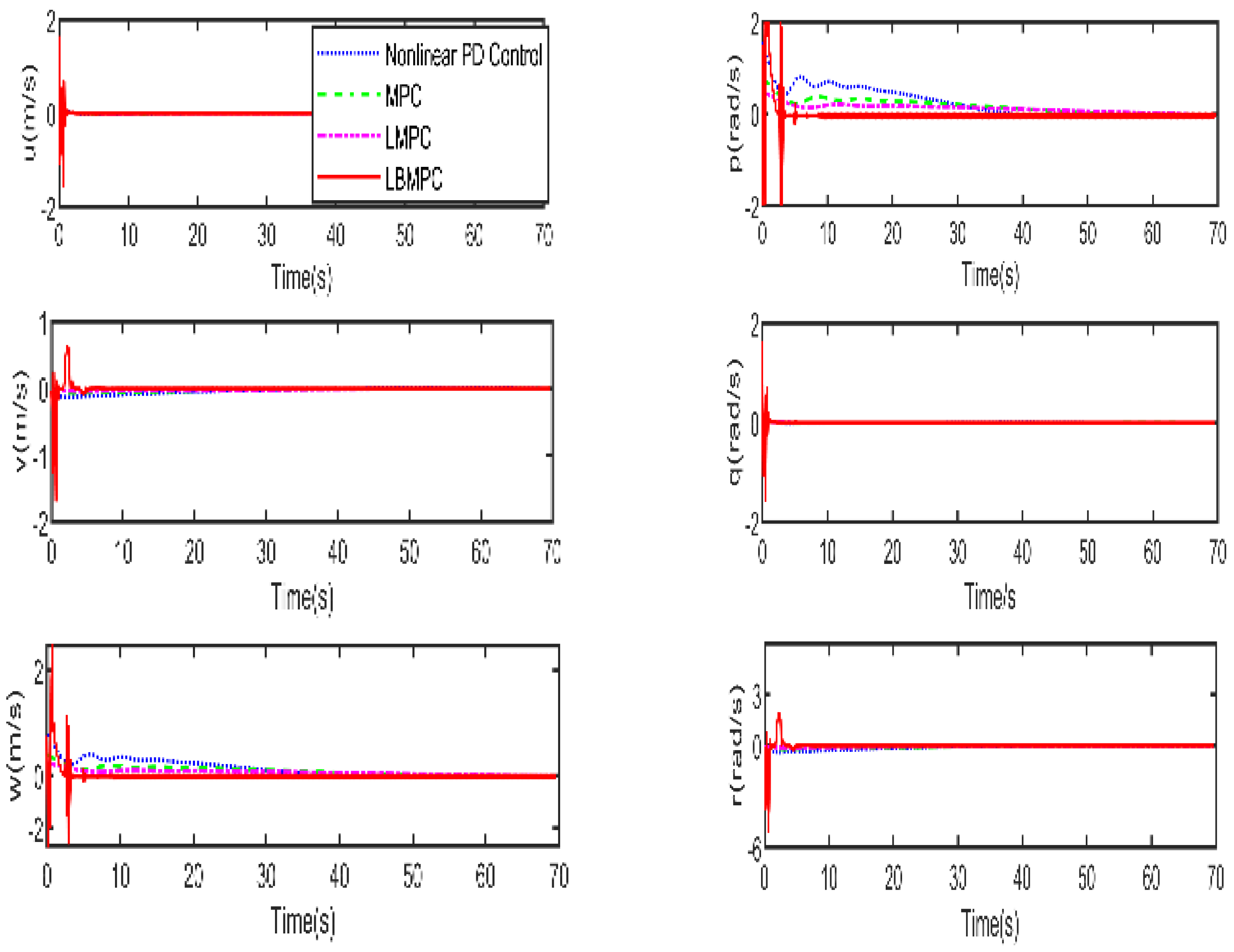
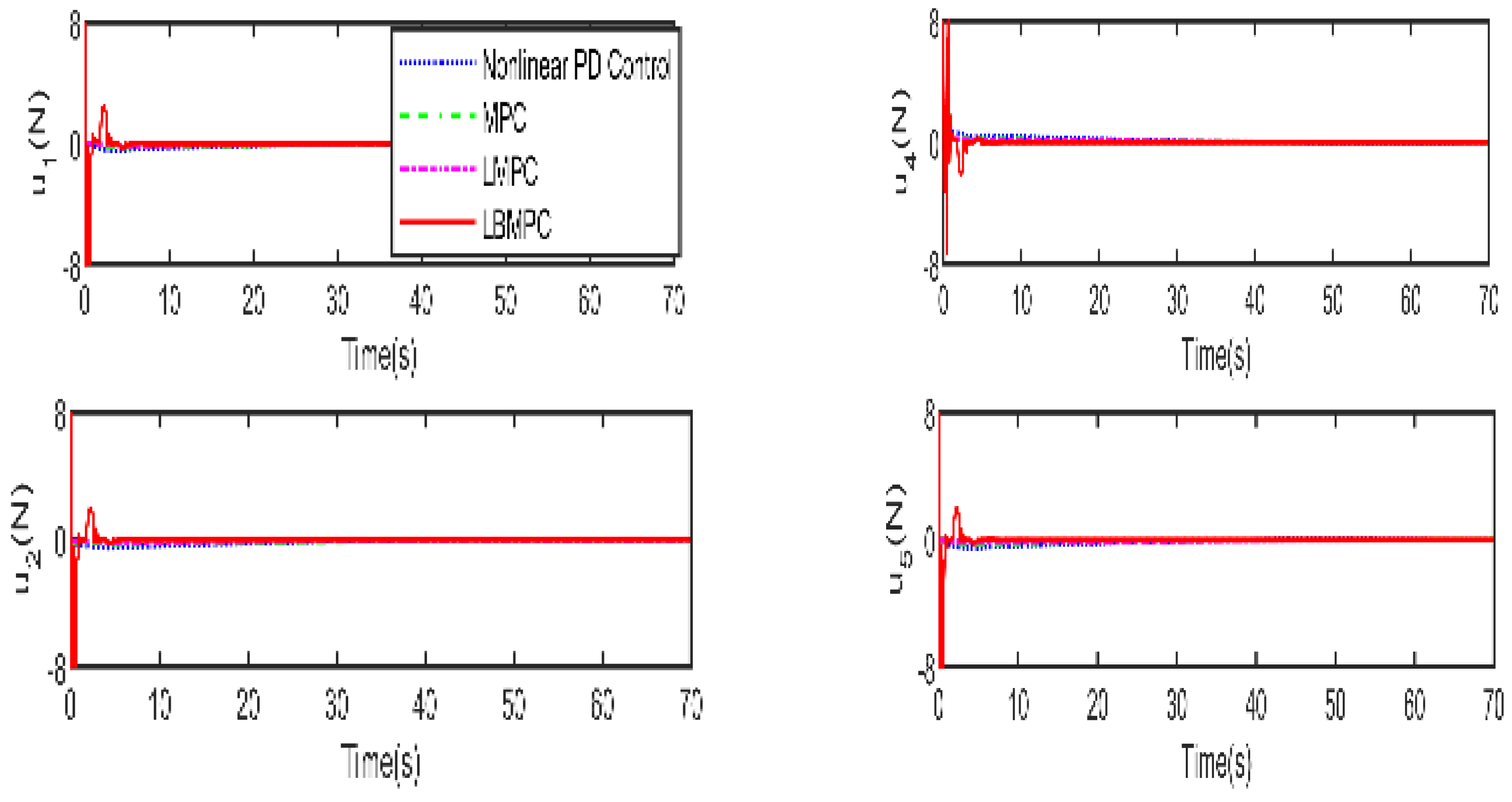
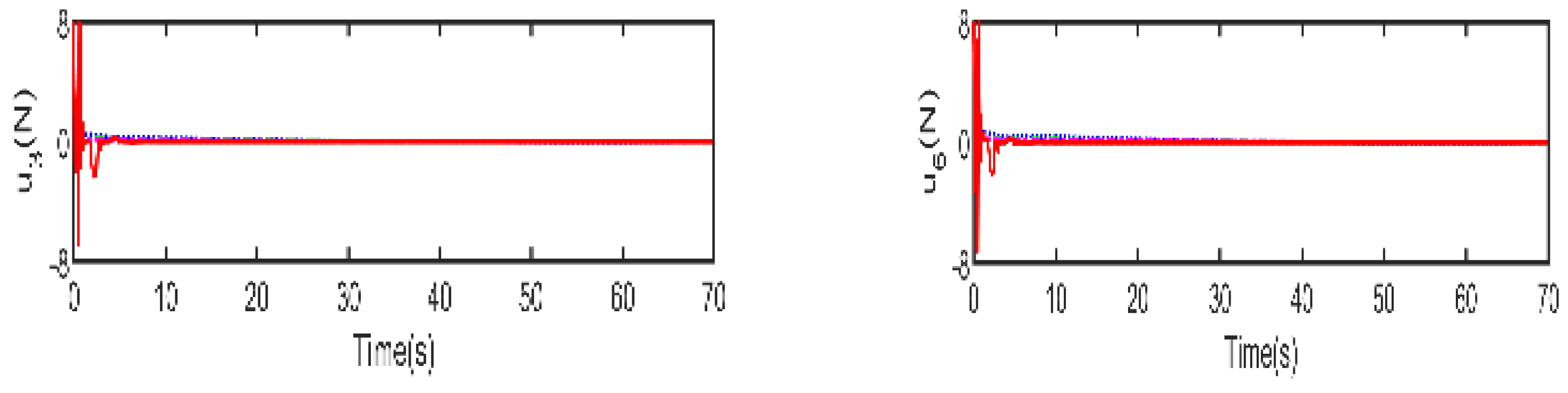
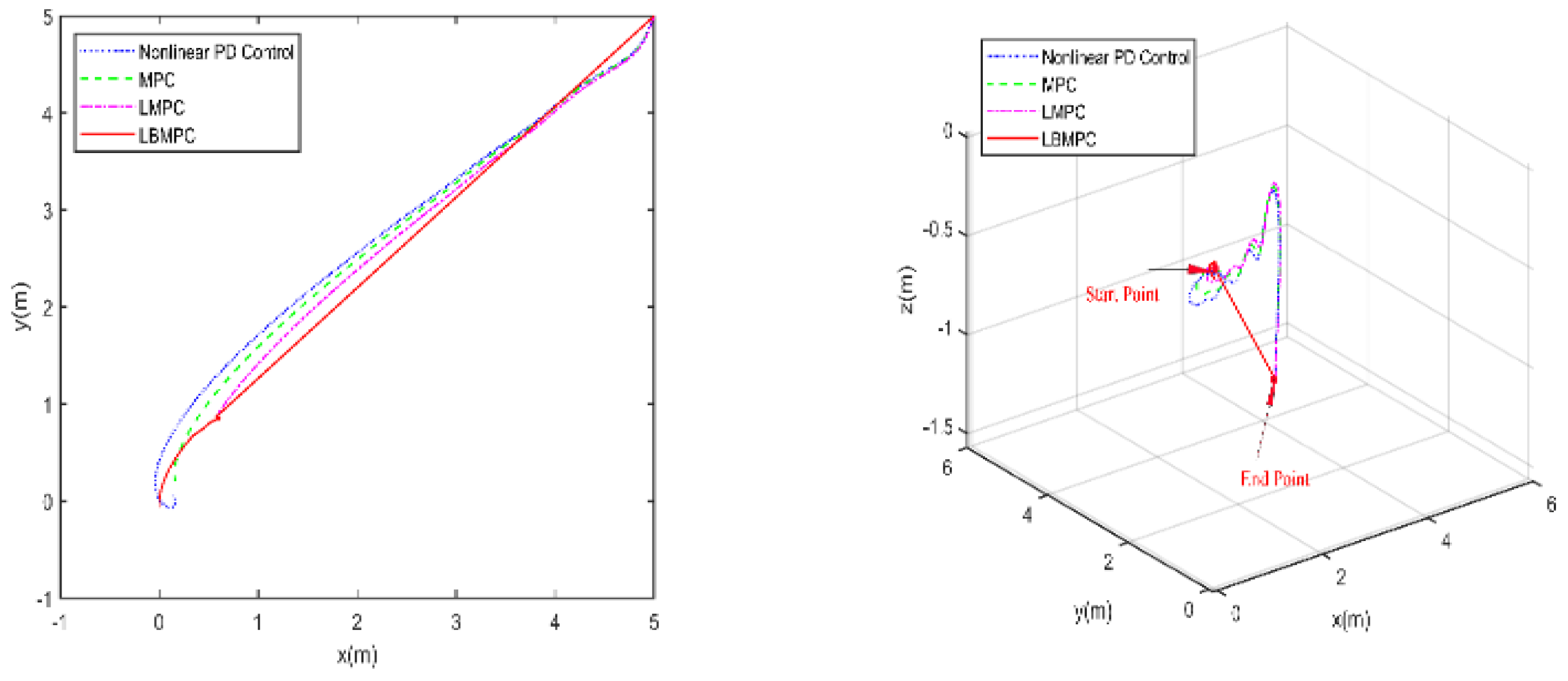
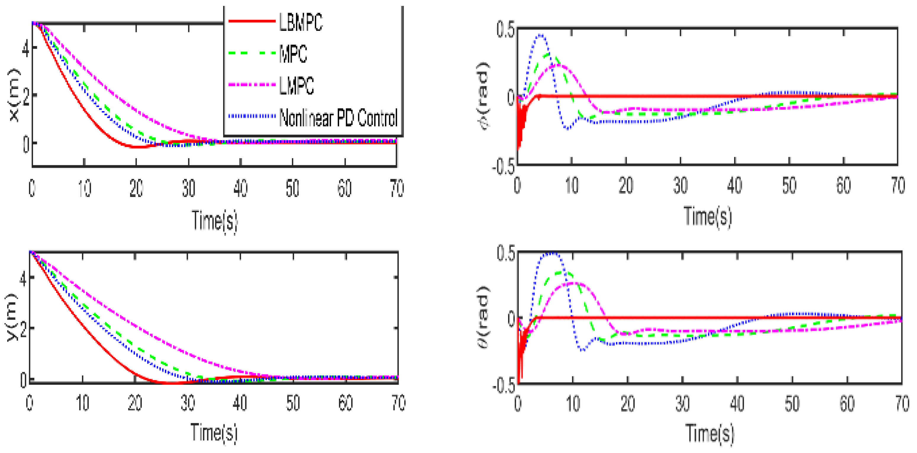
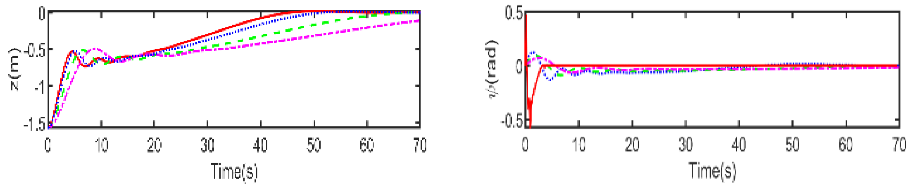
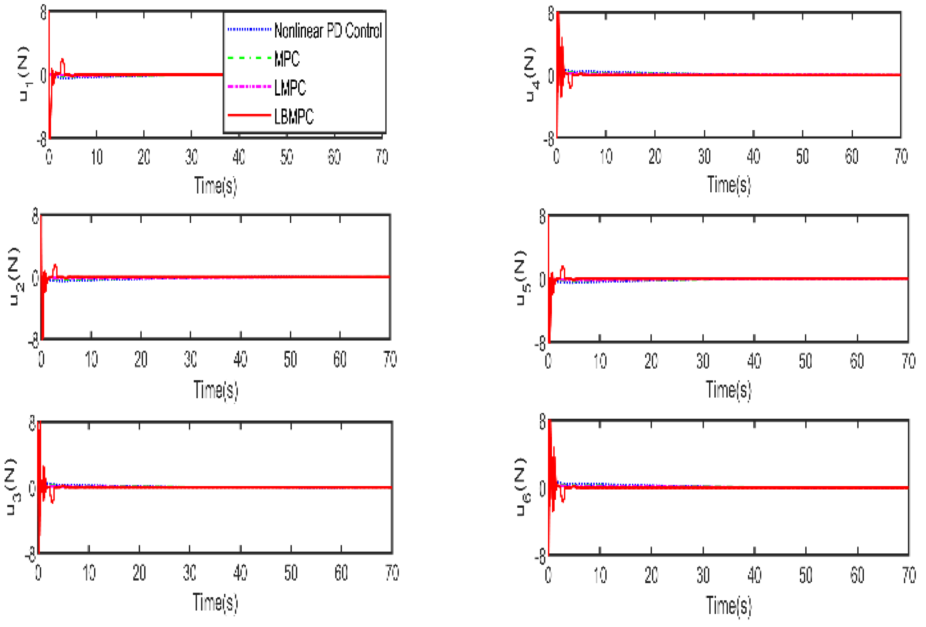
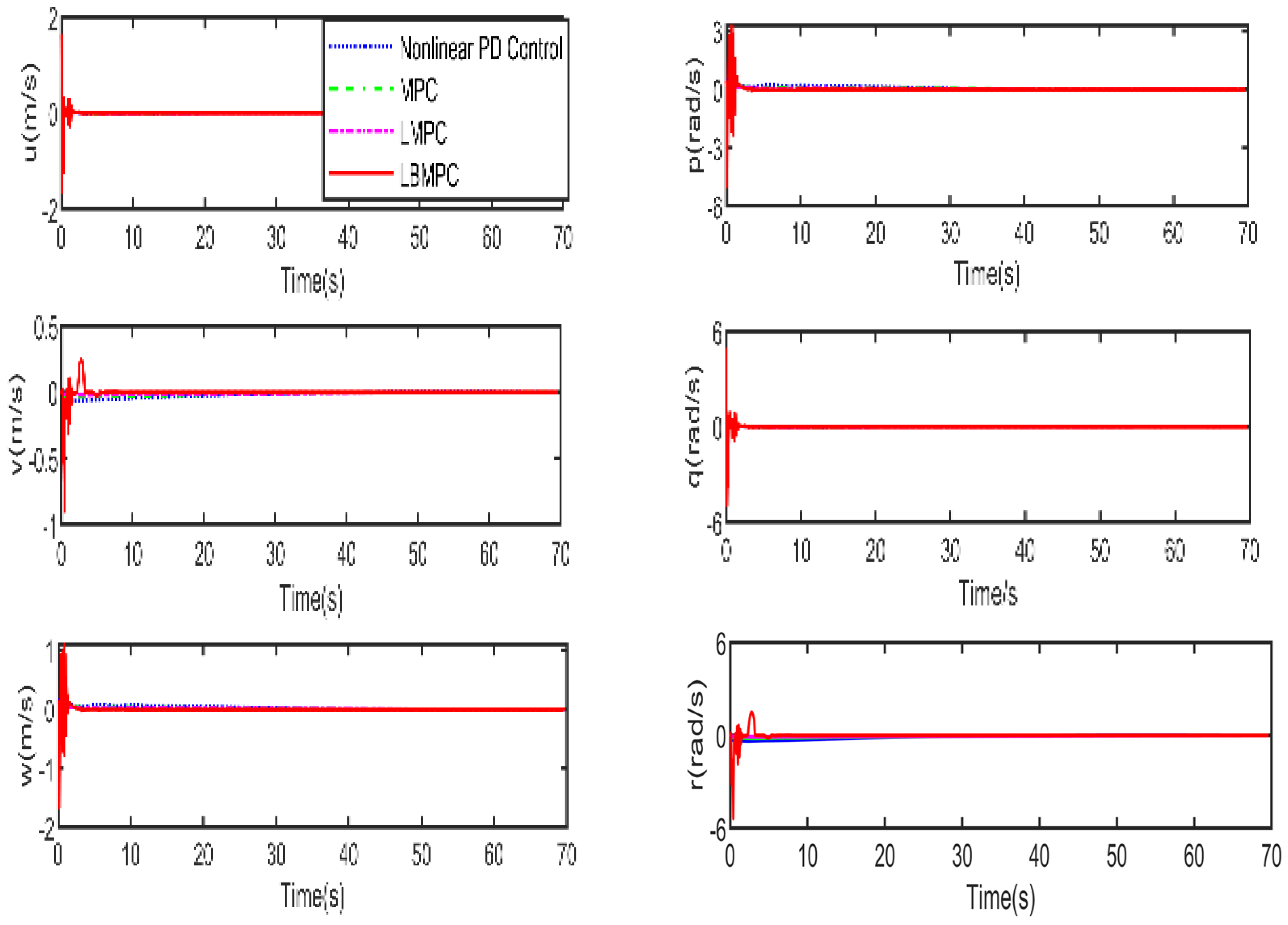
The first experiment was conducted without disturbances and uncertainties to observe the behavior of the proposed controller under ideal conditions. The trajectories towards the origin of the S-ASUV in 2D (left) and 3D (right) are shown in Figure 3, and Figure 4 illustrates the responses involving the position x, y, z and, pose $\varphi ,\theta ,\psi$ of the vehicle. The corresponding linear and angular velocities $u,v,w,p,q,r$ are given in Figure 5. 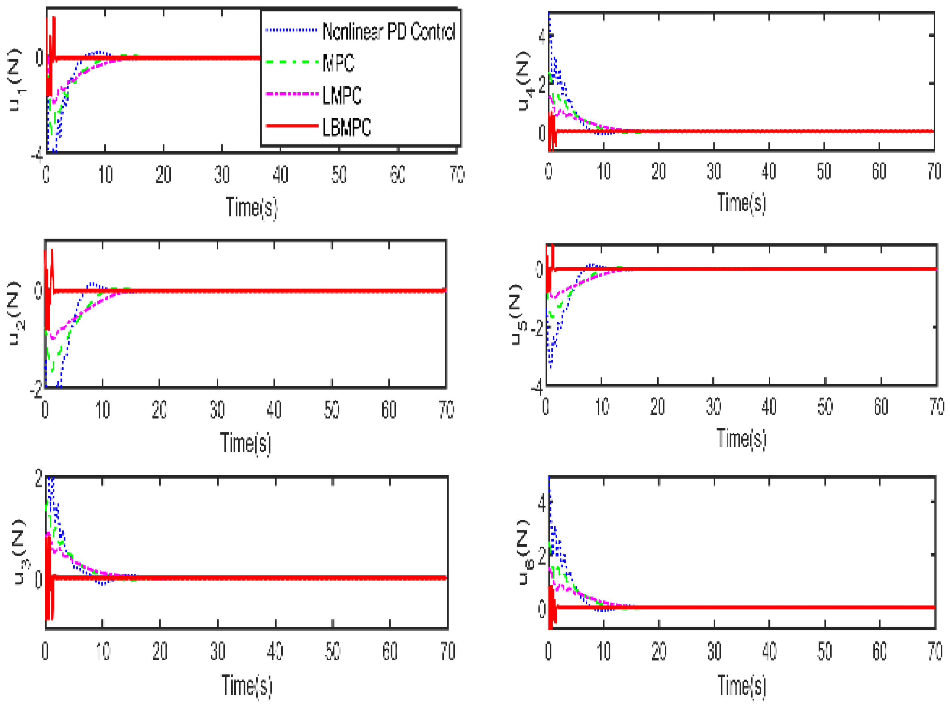As shown in Figure 6, which displays the thrust forces generated by individual propellers, it is confirmed that each control input stays within the designated permissible range as intended.

As shown in Figure 4 and Figure 5, it is clear that the LBMPC controller achieves a stable DP within the first 30 s, significantly quicker than the PD, MPC controller, and LMPC controller, which typically take around 45 to 55 s on average. The experiment results vividly demonstrate how real-time optimization improved the DP control performance. The results show that incorporating multi-variable PID secondary law led to a considerable enhancement in the convergence rate for DP control when utilizing the LBMPC method. This improvement is noticeable throughout a broad range of interactions.

3.2.2. Performance with Moderate Disturbances and Uncertainties

In the second experiment, depicted in Figure 7, Figure 8, Figure 9 and Figure 10, this study aimed to enhance the robustness of LBMPC. To emulate an irrotational ocean current, which exerts a consistent force on the vehicle, we introduced a disturbance index with a magnitude of ${\left[2;2;2;0;0;0\right]}^T$. Moreover, we included a 20% system model error to further assess the controller’s ability to cope with such intricate situations.

As shown in Figure 7, Figure 8, Figure 9 and Figure 10, which depict the outcomes under moderate disturbances and model uncertainties, the LBMPC controller maintained robustness. In Figure 7, using the proposed method reached the origin in the shortest route, while the other controllers needed longer ways. Looking at Figure 8 and Figure 9, the proposed method performed even better, achieving DP within 40 s, surpassing the PD, MPC and LMPC controllers, which took much more time to accomplish this task. The overall deviation when using LBMPC towards the origin over time is the smallest among the methods. It becomes clear that the LBMPC DP control not only achieves convergence to the desired target location but also improves overall performance, including robustness, accuracy and rapidity, of the DP control system.

3.2.3. Performance with Heavy Disturbances and Uncertainties

In the last experiment, depicted in Figure 11, Figure 12, Figure 13 and Figure 14, this work sought to reaffirm the robustness of the proposed controller. Introducing a heavy disturbance index of ${\left[4;4;4;0;0;0\right]}^T$ magnitude, we deliberately incorporated a +20% system model error and a −20% variation in the damping matrix to replicate the most demanding scenario. This was undertaken to assess the controller’s effectiveness in managing heavy scenarios and complex situations.

In the trajectory responses shown in Figure 11, the proposed LBMPC controller consistently outperformed other controllers by reaching convergence in the shortest route. This trend is further highlighted in Figure 12, where the proposed controller achieved DP significantly fastest, within 30 s. Additionally, the control inputs depicted in Figure 14 remained within the designated permissible range. Compared to the first two experiments, it is evident that the proposed control method performs best among the three different conditions.

4. Discussion

This inherent robustness is a notable advantage of LMPC and renders it an attractive option, particularly in marine control systems [22]. In the experiment results, the LBMPC controller demonstrates sustained robustness. It not only achieves convergence to the desired target location but also enhances the overall robustness of the DP control system, even under the most challenging scenarios. As mentioned earlier, the dynamic response’s rapidity and robustness are significant for the DP problem in marine vehicles. By incorporating the designed PID feedback into a closed-loop system, the proposed LBMPC improves the accuracy and rapidity of the DP control responses significantly compared to both the conventional LMPC and commonly used approaches, improving the DP control performance of marine vehicles, including S-ASUV in complex dynamic environments.

Beyond validation, the experiments using the S-ASUV model offered cost and time efficiencies, allowing extensive testing and scenario exploration in a virtual environment, thereby mitigating risks associated with actual operations. It enables iterative refinement of the proposed control method, rapidly incorporating improvements to enhance the S-ASUV’s performance while collecting comprehensive data for in-depth analysis of system behavior and informed decision-making. Ultimately, the series of experiments serves as a vital tool, optimizing and validating the proposed LBMPC framework, critical for precise motion control in complex underwater environments.

This study acknowledges several limitations that need to be addressed for a comprehensive understanding and application of the proposed methods. Firstly, the digital experiments were conducted under idealized conditions that may not fully replicate real-world environments, necessitating future testing in more varied and challenging scenarios to validate the robustness of the control strategies. Hydrodynamic modeling relies on specific assumptions about environmental forces and vehicle dynamics, which may not hold true in all operational contexts and could potentially affect control system performance. The practicality of the proposed control law is limited by its inclusion of terms for environmental disturbances and uncertain hydrodynamic forces, which are not directly measurable in real-world applications, indicating a need for additional estimation or compensation methods. While the digital experiment results are promising, they do not substitute for field tests; actual deployment on autonomous underwater vehicles in various operational conditions is necessary to thoroughly evaluate the system’s effectiveness and reliability. Additionally, the control system’s performance may be sensitive to the tuning of specific parameters, requiring a systematic study of parameter sensitivity and the development of robust tuning methods to ensure consistent performance. Lastly, the study does not address the long-term stability and adaptability of the control system in dynamic and unpredictable environments, highlighting the need for future work on adaptive control mechanisms that can adjust to changing conditions over extended periods.

5. Conclusions

This research introduces a novel LBMPC method providing an innovative solution to the challenging problem of three-dimensional DP for S-ASUVs. The proposed methodology incorporates a multi-variable PID controller into the secondary control law, effectively addressing external disturbances and model uncertainties. This approach demonstrates significant advantages over existing classical and modern DP techniques, particularly in accuracy, robustness, and responsiveness.

The feasibility and stability of the LBMPC algorithm are rigorously proven. The system guarantees recursive feasibility and continuous stability of the required equilibrium point, ensuring reliable performance in dynamic and uncertain marine environments.

A comprehensive series of experiments conducted using the S-ASUV model under diverse conditions confirm the proposed method’s superiority. The results showcase its robustness and rapidity for achieving precise 3D dynamic positioning, even in complex operational scenarios.

The contributions of this study extend beyond S-ASUVs, offering a robust control framework applicable to other marine vehicles, such as deep-sea ARVs. This research not only addresses critical challenges in 3D DP control but also sets a strong foundation for future studies, including real-world validation and cooperative control applications for multiple autonomous vehicles.