Figure 1.
Comparison of P300 and non-P300 waveforms.
Figure 1.
Comparison of P300 and non-P300 waveforms.
Figure 2.
Character matrix in the row-column paradigm.
Figure 2.
Character matrix in the row-column paradigm.
Figure 3.
Detailed structure of the improved inception module. The four parallel layers, denoted as , , , and , are concatenated at the end to form a unified feature representation.
Figure 3.
Detailed structure of the improved inception module. The four parallel layers, denoted as , , , and , are concatenated at the end to form a unified feature representation.
Figure 4.
Inception-CNN architecture, illustrating the inception layer, convolutional layer, and fully connected (FC) layer, along with the input and output feature maps (FMs). The circles in the FC layer represent neurons performing weighted sums followed by activation functions. The concatenated outputs of the inception layer before the spatial convolutional layer are denoted as , , , and , while those before the temporal convolutional layer are denoted as , , , and .
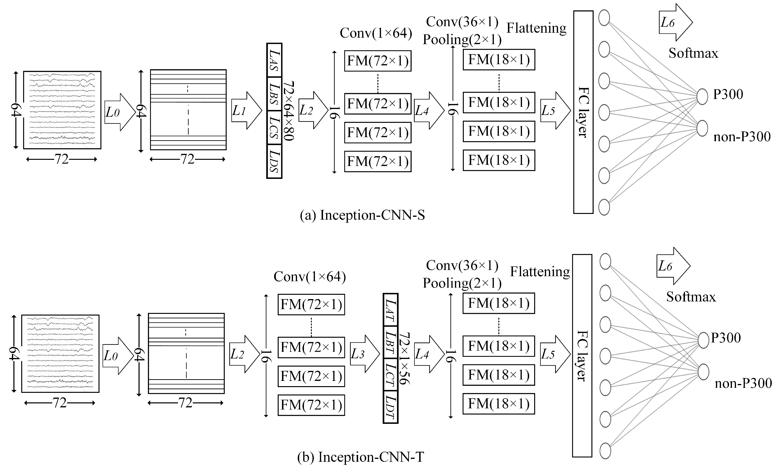
Figure 5.
(a) The structural composition of Inception-CNN-S, without the layer, and (b) the configuration of Inception-CNN-T, without the layer.
Figure 5.
(a) The structural composition of Inception-CNN-S, without the layer, and (b) the configuration of Inception-CNN-T, without the layer.
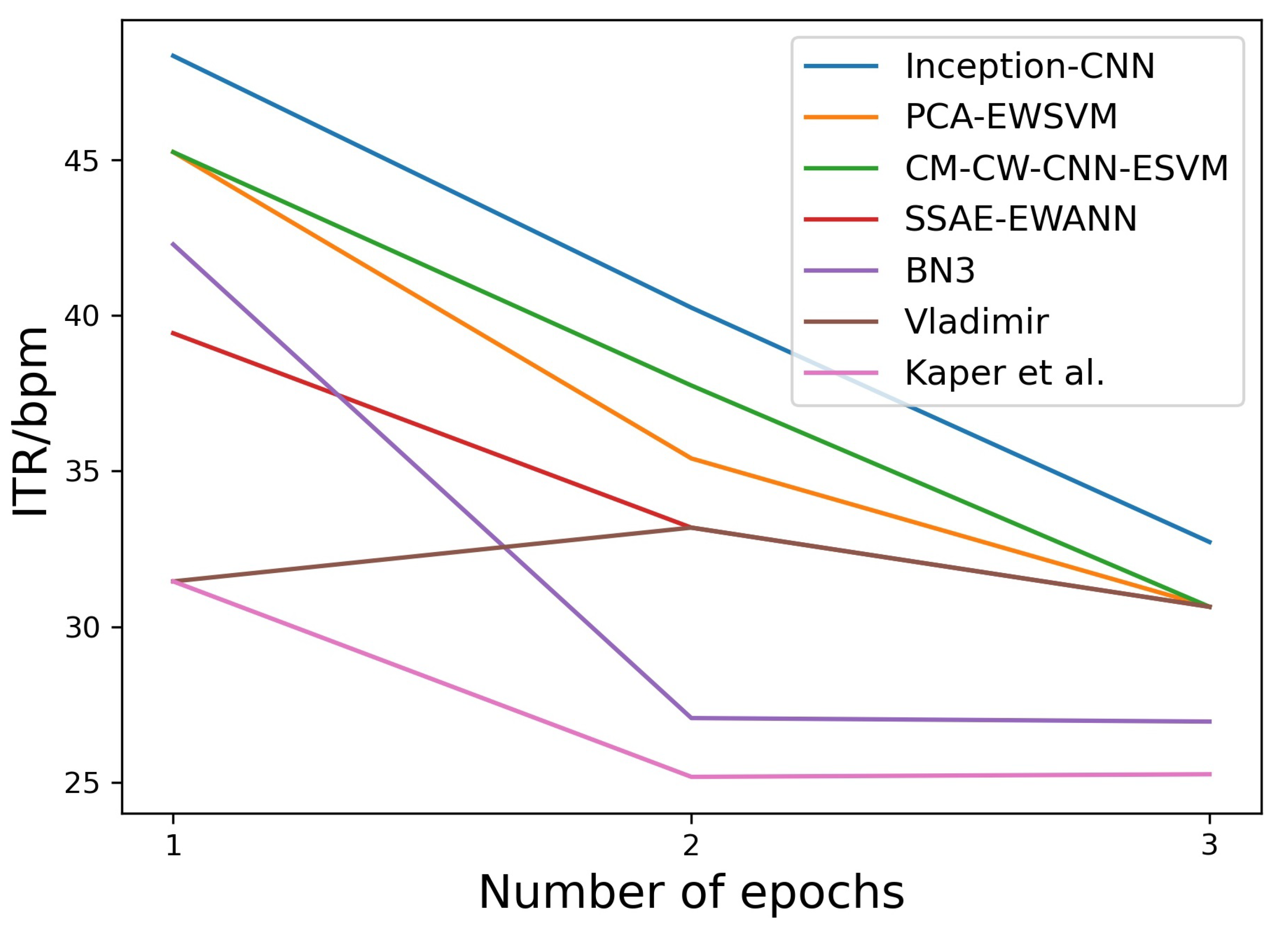
Figure 6.
Comparison of ITR of Inception-CNN with that of different models on the BCI IIIA and BCI IIIB datasets.
Figure 6.
Comparison of ITR of Inception-CNN with that of different models on the BCI IIIA and BCI IIIB datasets.
Figure 7.
Comparison of the ITR of the proposed Inception-CNN model with that of previously reported techniques on the BCI II dataset [
13].
Figure 7.
Comparison of the ITR of the proposed Inception-CNN model with that of previously reported techniques on the BCI II dataset [
13].
Table 1.
Number of samples in the training and test sets for BCI IIIA, BCI IIIB, and BCI II.
Table 1.
Number of samples in the training and test sets for BCI IIIA, BCI IIIB, and BCI II.
| Subject | Train | Test |
|---|
| P300 | Non-P300 | P300 | Non-P300 |
|---|
| BCI IIIA | 12,750 | 12,750 | 3000 | 15,000 |
| BCI IIIB | 12,750 | 12,750 | 3000 | 15,000 |
| BCI II | 6300 | 6300 | 930 | 4650 |
Table 2.
Overview of the Inception-CNN architecture. The architecture consists of seven layers, denoted as , , , , , , and . The kernel size, input size, number of features, and parameters in each layer are provided.
Table 2.
Overview of the Inception-CNN architecture. The architecture consists of seven layers, denoted as , , , , , , and . The kernel size, input size, number of features, and parameters in each layer are provided.
| Layer | Kernel Size | Input Size | Number of Features | Parameters |
|---|
| - | | - | 4 |
| (), ()(), ()(), () | | 80 | 18,072 |
| | | 16 | 81,936 |
| (), ()(), ()(), () | | 56 | 3856 |
| | | 16 | 32,272 |
| - | | 64 | 18,496 |
| - | 64 | - | 130 |
| Total | - | - | - | 154,766 |
Table 3.
Parameter details of the inception layer.
Table 3.
Parameter details of the inception layer.
| Layers | 1 × 1 | 3 × 3 | 5 × 5 |
|---|
| 24 | - | - |
| 24 | 16 | - |
| 24 | - | 24 |
| 16 | - | - |
| 24 | - | - |
| 16 | 8 | - |
| 8 | - | 8 |
| 16 | - | - |
Table 4.
Steps in the experimental setup, along with the descriptions and pseudocode for the BCI IIIA, BCI IIIB, and BCI II datasets.
Table 4.
Steps in the experimental setup, along with the descriptions and pseudocode for the BCI IIIA, BCI IIIB, and BCI II datasets.
| Step | Description | Pseudocode |
|---|
| | | Procedure start |
| 1 | Data Preprocessing | Load EEG data → Filter (0.1–20 Hz) |
→ Epoch Extraction (0–600 ms)
→ Downsample (240 Hz to 120 Hz) |
| 2 | Define CNN | Define CNN (Inception-CNN,
Inception-CNN-S, Inception-CNN-T) |
| 3 | Train Model | Use Keras Tuner to optimize
hyperparameters (e.g., filter sizes, learning rate) |
| Train each model using K-fold cross-validation |
| Evaluate models |
| 4 | P300 Detection | Predict P300/Non-P300 |
| 5 | Probability Calculation | Aggregate epoch probabilities |
| 6 | Character Mapping | Identify maximum probability row/column → Decode |
| 7 | Character Recognition | Map (row, column) → Display character |
| 8 | Accuracy Evaluation | Calculate F1 score and other metrics (P300/Non-P300)
Character recognition accuracy |
| Compare with other methods |
| | | End of procedure |
Table 5.
P300 detection results of the proposed methods compared with those of previously reported techniques on the BCI IIIA, BCI IIIB, and BCI II datasets. The results in bold represent the highest values.
Table 5.
P300 detection results of the proposed methods compared with those of previously reported techniques on the BCI IIIA, BCI IIIB, and BCI II datasets. The results in bold represent the highest values.
| Dataset | Method | TP | TN | FP | FN | Reco. | Recall | Precision | F1 Score |
|---|
| BCI IIIA | Inception-CNN | 1598 | 12819 | 2181 | 1402 | | | | |
| | Inception-CNN-S | 1515 | 12953 | 2047 | 1485 | | | | |
| | Inception-CNN-T | 1563 | 12598 | 2402 | 1437 | | | | |
| | BN3 [22] | 1910 | 11615 | 3385 | 1090 | | | | |
| | CNN-1 [20] | 2021 | 10645 | 4355 | 979 | | | | |
| | MCNN-1 [20] | 2071 | 10348 | 4652 | 929 | | | | |
| | MCNN-3 [20] | 2023 | 10645 | 4355 | 977 | | | | |
| BCI IIIB | Inception-CNN | 1712 | 13519 | 1481 | 1288 | | | | |
| | Inception-CNN-S | 1795 | 13007 | 1993 | 1205 | | | | |
| | Inception-CNN-T | 1847 | 12820 | 2180 | 1153 | | | | |
| | BN3 [22] | 2084 | 12139 | 2861 | 916 | | | | |
| | CNN-1 [20] | 2035 | 12039 | 2961 | 965 | | | | |
| | MCNN-1 [20] | 2202 | 11453 | 3547 | 798 | | | | |
| | MCNN-3 [20] | 2077 | 11997 | 3003 | 923 | | | | |
| BCI II | Inception-CNN | 778 | 4387 | 263 | 152 | | | | |
| | Inception-CNN-S | 749 | 4213 | 437 | 181 | | | | |
| | Inception-CNN-T | 733 | 3944 | 706 | 197 | | | | |
| | BN3 [22] | 752 | 3960 | 690 | 178 | | | | |
Table 6.
Character recognition accuracy of the proposed methods compared with that of previously reported techniques on the BCI IIIA and BCI IIIB datasets. The results in bold represent the highest accuracy.
Table 6.
Character recognition accuracy of the proposed methods compared with that of previously reported techniques on the BCI IIIA and BCI IIIB datasets. The results in bold represent the highest accuracy.
| Subject | Method | Number of Epochs |
|---|
| | | | | | | | | | | | | | |
|---|
| BCI IIIA | Inception-CNN | 22 | | 56 | | 70 | | | | | 90 | | | | | |
| | Inception-CNN-S | 20 | 42 | 52 | 58 | 72 | 73 | 76 | 82 | 87 | | 91 | 90 | 92 | 91 | 95 |
| | Inception-CNN-T | | 37 | 51 | 61 | 64 | 74 | 79 | 78 | 84 | 88 | 87 | 86 | 87 | 90 | 92 |
| | WE-SPSQ CNN [24] | 19 | 29 | 56 | 67 | | 70 | 76 | 77 | 83 | 86 | 88 | 91 | 94 | 93 | 98 |
| | CM-CW-CNN-ESVM [23] | 22 | 32 | 55 | 59 | 64 | 70 | 74 | 78 | 81 | 86 | 86 | 90 | 91 | 94 | |
| | SSAE-EWANN [19] | 21 | 35 | 54 | 64 | 67 | 72 | 74 | 76 | 83 | 89 | 89 | 93 | 92 | 95 | 98 |
| | BN3 [22] | 22 | 39 | | 67 | 73 | 75 | 79 | 81 | 82 | 86 | 89 | 92 | 94 | 96 | 98 |
| | CNN-1 [20] | 16 | 33 | 47 | 52 | 61 | 65 | 77 | 78 | 85 | 86 | 90 | 91 | 91 | 93 | 97 |
| | MCNN-1 [20] | 18 | 31 | 50 | 54 | 61 | 68 | 76 | 76 | 79 | 82 | 89 | 92 | 91 | 93 | 97 |
| | MCNN-3 [20] | 17 | 35 | 50 | 55 | 63 | 67 | 78 | 79 | 84 | 85 | 91 | 90 | 92 | 94 | 97 |
| | E-SVM [9] | 16 | 32 | 52 | 60 | 72 | − | − | − | − | 83 | − | − | 94 | − | 97 |
| BCI IIIB | Inception-CNN | 46 | | | 75 | | | | 91 | 93 | 94 | | 95 | 96 | | |
| | Inception-CNN-S | 43 | 54 | 64 | 71 | 81 | 84 | 86 | 88 | 89 | 92 | 91 | 92 | 91 | 93 | 94 |
| | Inception-CNN-T | 41 | 59 | 65 | 72 | 81 | 83 | 87 | 90 | 90 | 92 | 92 | 94 | 93 | 93 | 94 |
| | WE-SPSQ CNN [24] | 43 | 59 | 66 | | 78 | 83 | 89 | 89 | 89 | 93 | 92 | 92 | 91 | 92 | 91 |
| | CM-CW-CNN-ESVM [23] | 37 | 58 | 70 | 72 | 80 | 86 | 86 | 89 | 93 | | | | | | |
| | SSAE-EWANN [19] | 39 | 59 | 66 | 68 | 76 | 80 | 85 | 87 | 91 | 93 | 93 | 93 | 95 | 95 | 98 |
| | BN3 [22] | | 59 | 70 | 73 | 76 | 82 | 84 | 91 | | 95 | 95 | 95 | 94 | 94 | 95 |
| | CNN-1 [20] | 35 | 52 | 59 | 68 | 79 | 81 | 82 | 89 | 92 | 91 | 91 | 90 | 91 | 92 | 92 |
| | MCNN-1 [20] | 39 | 55 | 62 | 64 | 77 | 79 | 86 | | 91 | 92 | | 95 | 95 | 94 | 94 |
| | MCNN-3 [20] | 34 | 56 | 60 | 68 | 74 | 80 | 82 | 89 | 90 | 90 | 91 | 88 | 90 | 91 | 92 |
| | E-SVM [9] | 35 | 53 | 62 | 68 | 75 | − | − | − | − | 91 | − | − | 96 | − | 96 |
Table 7.
Character recognition accuracy of the proposed Inception-CNN model compared with that of previously reported techniques on the BCI IIIA and BCI IIIB datasets. The numbers in bold represent the best performance.
Table 7.
Character recognition accuracy of the proposed Inception-CNN model compared with that of previously reported techniques on the BCI IIIA and BCI IIIB datasets. The numbers in bold represent the best performance.
| Dataset | Epochs | PCA-EWSVM [11] | HOSRDA + LDA [16] | gsBLDA [17] | Data Partition-ESVM [37] | EFLD [38] | TSR [39] | WE-SPSQ CNN [24] | Inception-CNN |
|---|
| BCI IIIA | 10 | | | | | | − | | |
| | 15 | | | | | | | 98 | |
| BCI IIIB | 10 | | | | | | − | | |
| | 15 | | | | | | | | |
| Avg | 10 | | | | | | − | | |
| | 15 | | | | | | | | |
Table 8.
Results of paired t-test comparing the character recognition accuracy of Inception-CNN with that of other methods on the BCI IIIA and BCI IIIB datasets, including test-statistic (t-stat) and p-value.
Table 8.
Results of paired t-test comparing the character recognition accuracy of Inception-CNN with that of other methods on the BCI IIIA and BCI IIIB datasets, including test-statistic (t-stat) and p-value.
| Inception-CNN Paired with | t-Stat | p-Value |
|---|
| WE-SPSQ CNN | 5.650 | |
| CM-CW-CNN-ESVM | 5.193 | |
| SSAE-EWANN | 7.602 | |
| BN3 | 4.508 | |
| CNN-1 | 9.731 | |
| MCNN-1 | 7.977 | |
| MCNN-3 | 11.692 | |
| ESVM | 5.233 | |
Table 9.
Character recognition accuracy of the proposed Inception-CNN model compared with that of previously reported techniques on the BCI II dataset. The values in bold represent the highest values.
Table 9.
Character recognition accuracy of the proposed Inception-CNN model compared with that of previously reported techniques on the BCI II dataset. The values in bold represent the highest values.
| Subject | Number of Epochs |
|---|
| 1 | 2 | 3 | 4 | 5 | 6 |
|---|
| Inception-CNN | | | | 31 | 31 | 31 |
| SSAE-EWANN | 23 | 26 | 29 | 30 | 31 | 31 |
| CM-CW-CNN-ESVM | 25 | 28 | 29 | 31 | 31 | 31 |
| BN3 | 24 | 23 | 27 | 28 | 29 | 30 |
| PCA-EWSVM | 25 | 27 | 29 | 31 | 31 | 31 |
| Vladimir | 20 | 26 | 29 | 30 | 30 | 31 |
| Kaper et al. [13] | 20 | 22 | 26 | 30 | 31 | 31 |
Table 10.
The predicted characters in the first 4 epochs and the error (in %) of the proposed Inception-CNN model on the BCI II dataset. The characters in bold represent incorrectly predicted characters.
Table 10.
The predicted characters in the first 4 epochs and the error (in %) of the proposed Inception-CNN model on the BCI II dataset. The characters in bold represent incorrectly predicted characters.
| Epoch | Predicted Characters | Error |
|---|
| 1 | FOODMOOTHAMPIECAKETUHAZYAOTVAZ7 | 16.2% |
| 2 | FOODMOOTHAMPIECAKETUNAZYGOTF5Y7 | 6.4% |
| 3 | FOODMOOTHAMPIECAKETUNAZSGOT4567 | 3.2% |
| 4 | FOODMOOTHAMPIECAKETUNAZYGOT4567 | 0% |
Table 11.
Performance comparison of various methods on the BCI IIIA (Subject A) and BCI IIIB (Subject B) datasets in terms of mean F1 score and character recognition/ITR for epochs 5, 10, and 15. The best results in each column are highlighted in bold. A dash (-) indicates that the value was not reported in the respective paper.
| Method | Mean F1 Score | BCI IIIA | BCI IIIB | Mean |
|---|
| 5 | 10 | 15 | 5 | 10 | 15 | 5 | 10 | 15 |
|---|
| Inception-CNN | 0.5121 | 70/12.69 | 90/10.69 | 99/8.89 | 84/17.15 | 94/11.58 | 99/8.89 | 77.00/14.92 | 92.00/11.14 | 99.00/8.89 |
| WE-SPSQ CNN [24] | - | 75/14.20 | 86/9.87 | 98/8.69 | 78/15.14 | 93/11.35 | 91/7.54 | 76.50/14.67 | 89.50/10.61 | 94.50/8.12 |
| CM-CW-CNN-ESVM [23] | - | 64/10.99 | 86/9.87 | 99/8.89 | 80/15.79 | 95/11.81 | 99/8.89 | 72.00/13.39 | 90.50/10.84 | 99.00/8.89 |
| SSAE-EWANN [19] | - | 67/11.83 | 89/10.48 | 98/8.69 | 76/14.51 | 93/11.35 | 98/8.69 | 71.50/13.17 | 91.00/10.92 | 98.00/8.69 |
| BN3 [22] | 0.4925 | 73/13.59 | 86/9.87 | 98/8.69 | 76/14.51 | 95/11.81 | 95/8.17 | 74.50/14.05 | 90.50/10.84 | 96.50/8.43 |
| CNN-1 [20] | 0.47 | 61/10.18 | 86/9.87 | 97/8.51 | 79/15.47 | 91/10.91 | 92/7.69 | 70.00/12.82 | 88.50/10.39 | 94.50/8.10 |
| MCNN-1 [20] | 0.4647 | 61/10.18 | 82/9.11 | 97/8.51 | 77/14.83 | 92/11.13 | 94/8.00 | 69.00/12.50 | 87.00/10.12 | 95.50/8.26 |
| MCNN-3 [20] | 0.4727 | 63/10.71 | 85/9.68 | 97/8.51 | 74/13.89 | 90/10.69 | 92/7.69 | 68.50/12.30 | 87.50/10.19 | 94.50/8.10 |
Table 12.
Summary of P300 classification and character recognition results on the BCI II dataset. The table highlights the performance of the proposed Inception-CNN model, including the F1 score, character recognition rate, and ITR, compared to existing methods. The best results in each column are highlighted in bold. A dash (-) indicates that the value was not reported in the respective paper.
| Method | F1 Score | BCI II |
|---|
| 1 | 2 | 3 |
|---|
| Inception-CNN | 0.7894 | 83.87/48.32 | 93.54/40.24 | 96.77/32.71 |
| PCA-EWSVM [11] | - | 80.64/45.23 | 87.09/35.40 | 93.54/30.64 |
| CM-CW-CNN-ESVM [23] | - | 80.64/45.23 | 90.32/37.74 | 93.54/30.64 |
| SSAE-EWANN [19] | - | 74.19/39.42 | 83.87/33.18 | 93.54/30.64 |
| BN3 [22] | 0.6341 | 77.41/42.27 | 74.19/27.06 | 87.09/26.95 |
| Vladimir [15] | - | 64.51/31.45 | 83.87/33.18 | 93.54/30.64 |
| Kaper et al [13] | - | 64.51/31.45 | 70.96/25.17 | 83.87/25.26 |
Table 13.
Performance evaluation of Inception-CNN for P300 detection with five repetitions. The tests were conducted on a Tesla K80 GPU provided by Google Colab, and the average detection time across all repetitions is reported alongside the individual times.
Table 13.
Performance evaluation of Inception-CNN for P300 detection with five repetitions. The tests were conducted on a Tesla K80 GPU provided by Google Colab, and the average detection time across all repetitions is reported alongside the individual times.
| Dataset | t1 | t2 | t3 | t4 | t5 | Mean |
|---|
| BCI IIIA | 3.90 | 3.74 | 3.74 | 3.76 | 3.86 | 3.80 |
| BCI IIIB | 3.89 | 3.63 | 3.65 | 3.61 | 3.74 | 3.70 |
| BCI II | 3.62 | 3.72 | 3.60 | 3.61 | 3.59 | 3.63 |


