Article

Open-Set Automatic Modulation Recognition Based on Circular Prototype Learning and Denoising Diffusion Model

1
The 54th Research Institute of CETC, Shijiazhuang 050081, China
2
Hebei Key Laboratory of Electromagnetic Spectrum Cognition and Control, Shijiazhuang 050081, China
3
School of Artificial Intelligence, Xidian University, Xi’an 710071, China
*
Author to whom correspondence should be addressed.
Electronics 2025, 14(3), 430; https://doi.org/10.3390/electronics14030430
Submission received: 25 December 2024 / Revised: 19 January 2025 / Accepted: 20 January 2025 / Published: 22 January 2025

Abstract

:
Automatic modulation recognition (AMR) technology is a critical component of modern communication systems. However, conventional AMR methods based on the closed-set assumption struggle to detect unknown classes that may appear during testing. To address this limitation, this paper proposes an open-set automatic modulation recognition (OSAMR) framework, termed CPLDiff, that integrates circular prototype learning (CPL) with a denoising diffusion model (DDM) to detect unknown classes. The core idea of CPLDiff is to jointly leverage the class-level and instance-level information of the training samples. To achieve this, CPL is used to extract class-level information, while the diffusion model is employed to extract instance-level information. (1) Circular Prototype Learning: Prototype vectors are pre-optimized and fixed, and a bias radius is introduced to expand the feasible encoding space. (2) Denoising Diffusion Model: Noise is added to the sample, and the DDM is used to remove this noise. The probability of a sample belonging to a known class is proportional to the extent of noise removal. (3) Final Integration: The outputs of the CPL and the DDM are combined to perform OSAMR. We conducted comparative experiments and evaluated the proposed method using diverse metrics to ensure a comprehensive assessment of its effectiveness. The experimental results demonstrate that the CPLDiff method significantly improves the detection capability for unknown classes compared to state-of-the-art methods.

1. Introduction

Signal modulation technology plays a critical role in modern communication systems [1]. It converts low-frequency baseband signals into high-frequency radio frequency (RF) signals and uses variations in parameters such as frequency and amplitude to carry information, resulting in modulation schemes such as amplitude modulation (AM), frequency modulation (FM), phase modulation (PM), quadrature amplitude modulation (QAM), frequency shift keying (FSK), and phase shift keying (PSK). Different modulation schemes directly affect the transmission capacity and spectral usage efficiency of the communication systems.
Accurately identifying the modulation type of the received signal is essential for subsequent demodulation and information processing. While the transmitter and receiver agree on the modulation scheme in cooperative scenarios, no prior parameters of the transmitted signals, such as signal power, carrier frequency and phase offsets, timing information, and so on, are provided to the receiver in non-cooperative situations. The blind identification of modulation schemes is a major task for the receivers in such non-cooperative scenarios, which is referred to as the automatic modulation recognition (AMR) technology [1]. The key advantage of AMR lies in its ability to identify the modulation scheme of the received signal without any prior knowledge, increasing its importance in scenarios such as electronic warfare, spectrum monitoring [2], resource allocation [3], and cognitive radio [4].
In recent years, the rapid development of deep learning has provided a more efficient and robust solution for AMR. Deep learning-based methods leverage well-trained artificial neural networks (ANNs) to automatically extract discriminative features, and they first require labeled samples to train the artificial neural network, after which the trained network can be used to recognize unlabeled test samples [5,6]. During these two stages, most deep learning methods assume that the class set of the unlabeled test samples is consistent with that of the labeled training samples. This assumption is known as the closed-set assumption [1]. In terms of sample types, researchers [7] have classified them into the following two categories:
  • Known Known Classes (KKCs): Classes for which we know that labeled samples exist during the training phase.
  • Unknown Unknown Classes (UUCs): Classes for which no information is available during the training phase.
Based on this definition, the closed-set assumption means that both test samples and training samples belong to the set of KKCs.
AMR methods based on the closed-set assumption typically fail to hold in today’s complex and diverse communication environments, where signals may belong to an entirely new modulation type. This scenario is referred to in academia as the open-set scenario: only KKC samples are available during the training phase, but both KKC and UUC samples may appear during the testing phase. When faced with UUC samples, AMR methods based on the closed-set assumption will incorrectly classify them as one of the KKCs. This overconfidence over UUC samples can be critical in fields such as access control and electronic warfare. Open-set automatic modulation recognition (OSAMR) is an emerging technology for open-set scenarios, and its differences with close-set AMR are shown in Table 1. In addition to classifying KKC samples, OSAMR is required to detect UUCs. The ability to reject UUCs makes OSAMR a key technology for applications such as authorization, monitoring, and adversarial scenarios [8,9,10]. Furthermore, OSAMR is an important step toward achieving adaptive modulation recognition systems, of which its goal is to enable autonomous learning and recognition. The overall process of adaptive modulation recognition systems involves certain tasks: novelty discovery [11], labeling, and class incremental learning [12,13]. OSAMR technology plays a crucial role in the novelty discovery task, and its performance directly impacts the subsequent learning steps.
The main constraint of open-set recognition lies in that only KKC samples are available during the training phase [7,14], and algorithms must be developed based solely on these samples to effectively detect UUCs. Under this constraint, some methods [15,16], based on metric learning, aim to achieve compact embeddings of the samples to reduce the overlap probability between KKCs and UUCs. Other methods use generative adversarial networks (GANs) [17] to simulate fake UUC samples, enhancing the recognition model’s ability to understand the open world. Additionally, some methods [18,19] approach the problem from a reconstruction perspective, where the reconstruction error for KKC samples is intuitively smaller than that for UUC samples. Given the inherent limitations of open-set tasks and the shortcomings of existing methods, the main challenges of OSAMR are summarized as follows:
  • How to fully utilize the KKC samples during training remains the key challenge of OSAMR, as only these samples are accessible. UUC samples that appear in testing are invisible during the training phase. According to the information bottleneck theory [20], any supervised learning is to extract minimal but sufficient statistics with respect to the objective function. Therefore, methods that adopt metric learning may suffer significant information loss. Meanwhile, methods attempting to simulate UUC samples offer limited and uncertain benefits as the number of UUCs is unknown and could be extremely large. The key to achieving OSAMR lies in fully extracting the information from the training samples.
  • How to enhance the detection capability for UUCs while maintaining the recognition accuracy of KKCs. In open-set recognition tasks, improving the UUC detection performance is often achieved at the cost of the recognition accuracy of KKCs. In other words, an improvement in one of performance typically results in a decline in the other. The ideal open-set recognition technology would achieve a higher detection rate for UUCs at the expense of only a slight reduction in the KKC recognition accuracy.
To address the above challenges, we propose CPLDiff, an OSAMR method designed to fully exploit the information carried by the training samples and achieve a higher UUC detection capability at a low cost in KKC recognition accuracy. The core idea of CPLDiff is quantifying two levels of information by extending circular prototype learning with a diffusion model. The former primarily focuses on class-level information by discovering the differences among KKCs and enriching the feature distribution. The latter learns the unique characteristics of individual samples to extract instance-level information. In particular, the diffusion model, by gradually adding and then removing noise, can achieve better reconstruction and generation results. OSAMR is achieved using similarity scores obtained from circular prototype learning and denoising scores derived from the diffusion model. In summary, the main contributions of CPLDiff are as follows:
  • We enhance prototype learning by optimizing and fixing each prototype and encouraging samples to surround their corresponding prototype in a circular manner. This approach is termed circular prototype learning (CPL).
  • We propose a diffusion model-based OSAMR strategy, where a certain amount of noise is randomly added to the samples. The probability of a sample belonging to the KKCs is proportional to the amount of noise removed by the diffusion model.
  • We extend circle prototype learning with the diffusion model to more fully exploit the information in the training samples and jointly utilize both methods for the combined prediction of the samples.

2. Related Works

2.1. Traditional Automatic Modulation Recognition

Traditional automatic modulation recognition (AMR) techniques can be categorized into two categories: likelihood-based (LB) and feature-based (FB) methods [1]. The former compute the likelihood function [21] of the signal and match it to the maximum likelihood value, while the latter extract features from the signal, such as high-order cumulants [22], and utilize machine learning classifiers for recognition [22,23]. Likelihood-based recognition methods are computationally complex and require perfect channel-state information (CSI) [24] at the receiver end. Feature-based methods rely on features manually designed by experts in the signal domain. With the rapid advancement of communication technology and the increasing complexity of communication environments, traditional AMR techniques face significant challenges. Their low robustness makes them increasingly inadequate for diverse modulation schemes and complex communication environments.

2.2. Deep Learning-Based Automatic Modulation Recognition

Deep learning-based AMR methods can be categorized based on the types of artificial neural networks, including convolutional neural network (CNN) models [25,26,27,28,29,30], Long Short-Term Memory (LSTM) models [31], Transformer models [32,33], and hybrid models [34,35,36]. They can also be classified according to the type of inputs, such as raw IQ inputs, transformed inputs (e.g., statistical features, spectrograms, constellation diagrams), and mixed inputs. Additionally, they can be divided based on the learning approaches, including supervised, semi-supervised [37], and self-supervised learning [38]. In the early stages of research, ref. [25] employed VGG networks with raw IQ data as input, achieving promising results for modulation recognition. Liu et al. [27] proposed a new DL-AMR model based on Residual Neural Networks (ResNet) and DenseNet, allowing features learned from multiple layers to be effectively transferred to the classification module. In [26], to better adapt a 2D-CNN to the sequential signals, the S2M operator was introduced to convert time-series signals into 2D square matrices. To incorporate additional expert knowledge of the signal, ref. [39] integrated the instantaneous features of the signal into the CNN input and demonstrated the effectiveness of expert knowledge in improving performance. Rajendran et al. [40] transformed the I-Q signals into amplitude and phase and fed them into an LSTM network, which achieved high recognition accuracy. CNN models typically focus on spatial features, while LSTM models focus on temporal features, and combining both may lead to enhanced recognition performance. MCLDNN [34] combines 1D-CNNs, 2D-CNNs, and LSTM, achieving more efficient feature extraction and faster convergence speed. Ref. [38] constructed a contrastive learning model using two modalities of signals, time-series data and constellation diagrams, and transferred the encoder weights to downstream classification and clustering tasks, thus expanding feasible pathways for AMR technology.

2.3. Open-Set Recognition

Open-set recognition was first introduced by Scheirer et al. in [7], where the task definition was clarified and a simple OSR framework was proposed. Over years of development, OSR methods can generally be divided into two categories: discriminative model-based methods and generative model-based methods [14,41].
Discriminative Models. Discriminative models focus primarily on learning the information that enables each KKC to be differentiated from each other. Early research by Hendrycks et al. [42] proposed a simple OSR baseline that uses the maximum SoftMax probability from a neural network as the sample score. To detect UUC samples, a threshold is determined practically or computationally. Bendale et al. [43] analyzed the limitations of the SoftMax function and thus proposed the OpenMax function as a replacement for SoftMax. OpenMax adjusts the logits using the mean activation vector (MAV) and a Weibull distribution. This approach does not require modifications to the network structure or the training loss function, making it simple and easy to implement, but with higher computational complexity. Another feasible approach is to increase the number of neurons in the network’s output layer, which is taken by Proser [44]. Proser increased the number of output neurons from C to C + N , where C represents the number of KKC, and N represents the number of classifier placeholders. Classifier placeholders simulate the center for UUC samples, activating the highest value when the input is from a UUC and the second-highest when it originates from one of the KKCs.
Another promising research area is prototype learning, which belongs to the family of discriminative models. Prototype learning uses prototype points to represent class centers and assumes samples are located closer to their belonging prototype. The first work to combine prototype learning with deep learning was GCPL [16]. It was aimed at enabling neural networks to extract more robust and discriminative representations, which can enhance performance in closed-set recognition, open-set recognition, and incremental learning. More recent works include RPL [45] and its improved version, ARPL [15]. RPL uses a reciprocal point (RP) to represent the otherness of a single KKC, such that training samples are pushed away from their corresponding RP, while samples from other classes (including UUCs) are pulled closer to the RP. ARPL further enhances the performance of RPL by imposing a radius between the RP and its KKC samples.
Generative Models. Generative models achieve open-set recognition through two independent approaches. The first involves generating fake samples to assist discriminative models in understanding the open world, while the second embeds original samples and then performs reconstruction. G-OpenMax [46] enhances OpenMax with an additional GAN and adds an extra activation neuron to represent the UUCs. OSRCI [47] follows a similar approach to G-OpenMax, where the generated fake samples need to resemble a specific KKC class. These fake samples then serve as the boundary between KKCs and UUCs. Similarly, ARPL+CS [15] generates confusing samples to stand for UUCs. Based on the reconstruction error, C2AE [18] was the first to use an autoencoder for OSR. C2AE trains an encoder on a closed-set classification task and fixes its weights. It then decodes and reconstructs the features extracted by the encoder. Since the encoder is trained for a classification task, the feature vectors it produces lack sufficient information to support effective reconstruction. CROSR [19] recognized this limitation of C2AE and addressed it by performing both classification and reconstruction tasks simultaneously.

3. Materials and Methods

3.1. Problem Definition

In this subsection, we provide a concise yet clear explanation of the open-set recognition task. Given a C-KKC classification task and an available training dataset,
D t r = { ( x 1 , y 1 ) , ( x 2 , y 2 ) , ( x n , y n ) } ,
where y i { 1 , 2 , , C } is the label of x i , and n is the size of the training dataset. And with an unlabeled testing dataset
D t e = { ( x 1 ) , ( x 2 ) , , ( x m ) } ,
where m is the number of testing samples, the goal of OSR is to correctly label each sample in D t e . The true label of any test sample belongs to the set { 1 , 2 , , C , C + 1 , , C + U } , where U is the number of UUCs. As U is unclear in testing, an OSR algorithm needs to label any sample of the KKCs with { 1 , 2 , , C } and any sample of UUCs with { C + 1 } , which means a rejection for classification. The performance of an OSR algorithm is determined by both the identifying accuracy for KKCs and the rejection rate for UUCs.

3.2. Overview

We display the proposed circular prototype learning and diffusion model (CPLDiff) OSAMR workflow in Figure 1. The framework is composed of the following three modules:
  • Circular prototype learning for the close-set prediction and similarity score.
  • Denoising diffusion model for denoising the score.
  • Score integration and prediction calibration.
A detailed explanation of the workflow for the proposed CPLDiff framework is as follows. First, CPL optimizes the location of prototype points, ensuring they are evenly distributed in the latent space. Once optimized, the prototype points are fixed, meaning their positions do not update during the training process. CPL then extends the optimal representation z (obtained through the encoding of the input signal s ) from the prototype point to a circular region around it. This extension enriches the information contained in z and prevents excessive information loss during the encoding process. Based on the distance between z and each of the circular regions, CPL outputs a distance score S 1 and a closed-set prediction y ¯ (Section 3.3). Recognizing the sample’s belonging class solely based on CPL only utilize the class-level information contained in the sample. To further verify the prediction results output by CPL, a score calculation method based on the denoising diffusion model (DDM) is attached after CPL. We add a certain amount of random noise to the original signal s and use the diffusion model to remove the noise. The extent of noise removal is quantified as a score S 2 , which reflects the instance-level information, and the probability that the sample belongs to the KKCs is proportional to this score (Section 3.4). Finally, scores S 1 and S 2 are weight-summed to obtain the final score, which is then used to correct the closed-set prediction result y ¯ (Section 3.5).

3.3. Circular Prototype Learning

3.3.1. Data Process and Encoding

One complex-value modulation signal can be denoted as
s ( t ) = s i ( t ) + j · s q ( t ) ,
where s i ( t ) and s q ( t ) represent the in-phase (Real) and quadrature (Image) components at time t { 1 , 2 , 3 , , L } , and L is the sampled length of the signal. As the signal has two channels, it is generally stored in a computer file system in a matrix manner as
s = s i s q ,
where s i = [ s i ( 1 ) , s i ( 2 ) , , s i ( L ) ] , and s q = [ s q ( 1 ) , s q ( 2 ) , , s q ( L ) ] . To eliminate the effects caused by fluctuations in the output power of the signal transmitter, we normalize the power of the signals according to the following formula:
s = s s t d ( s ) ,
where the s t d ( · ) function calculates the standard deviation of elements in matrix s . The normalization computational overhead is proportional to the matrix size. In real-world environments, the signals’ amplitude may vary in a wide range; thus, conducting normalization helps avoid gradient explosion and achieve a fast convergence speed. In addition to normalizing the signal power, we enhance the signal diversity by introducing the Givens transform [48] during the preprocessing stage, which is formulated as s ( t ) = ( s i ( t ) + j · s q ( t ) ) · exp ( j · ϕ ) or in a matrix manner as
s i s q i = cos ϕ sin ϕ sin ϕ cos ϕ s i s q ,
where ϕ [ 0 , 2 π ) is the rotation angle. Modulation signals are complex-valued signals, where the real part represents the in-phase channel, and the imaginary part represents the quadrature channel. Applying a Givens transform to a modulation signal effectively rotates the original complex signal clockwise around the origin of the complex plane and generate more signals with varying initial phases but identical modulation types. This online data augmentation, like cropping, scaling in the CV domain, increases the model’s robustness and is not unnecessary for test samples.
To encode a signal into a latent representation, we use a convolutional neural network (CNN) as the encoder, which is formulated as
z = L 2 ( f θ ( s ) ) ,
where f θ ( · ) denotes SigRes34 [38], a CNN model, L 2 ( · ) is the L2 normalization function, and z R 1 × D is the representation vector of s . L2 normalization is adopted on the raw encoded representation to simplify the distance metric into cosine similarity. Moreover, L2 normalization constrains the feature representation into a hyper-surface, making it possible for the next prototype pre-optimization.

3.3.2. Prototype Pre-Optimization

In this section, we introduce the rationale and methodology behind the pre-optimization (PPO). The classic prototype learning method, GCPL, assigns a prototype vector to each KKC, denoted as { P 1 , P 2 , , P C } , where the values of these prototype vectors are set as learnable parameters, meaning their locations are continuously updated throughout the training process. The loss function of GCPL consists of a cross-entropy loss and a center loss, both of which focus on minimizing the distance between prototypes and samples. However, they do not consider the relative distances between the prototype vectors themselves. After updates, some prototype vectors may end up being far apart, while others are close to each other. This imbalance results in the open-set risk being focused more on the prototype vectors that are closer together. Therefore, in addition to considering the sample-to-prototype distance, the prototype-to-prototype distance should also be taken into account.
PPO is proposed to address the issue of neglecting the prototype-to-prototype distance. First, PPO assumes that the distribution of prototype vectors in the feature space should be uniform, which helps evenly distribute the open-set risk across all prototype vectors. Second, the distribution of prototype vectors should be discrete, which helps reduce the open-set risk. Therefore, prior to training the encoder on the training set, the distribution of the prototype vectors is optimized. According to the main ideas of PPO, the designed loss function is
L p = 1 C × C j = 1 C k = 1 C CosineSim ( P j , P k ) ,
CosineSim ( x 1 , x 2 ) = x 1 · ( x 2 ) T max ( x 1 2 · x 2 2 , ϵ ) .
The function CosineSim ( · , · ) calculates the cosine similarity between the inputs, as defined in Equation (9), and ϵ is introduced to prevent division by zero. When minimizing Equation (8), the average similarity between prototype vectors is minimized, or in other words, the average distance is maximized. Since the prototype vectors are constrained on a convex hyper-sphere through L2 normalization, the minimum value of Equation (8) is attained only when all prototype vectors are uniformly distributed on the hyper-sphere. After PPO, all prototype vectors are fixed and no longer updated during the subsequent encoder training process. While other methods, such as GCPL and SoftMax, jointly train their encoders and classifiers, our separate training strategy does not include more computation overhead than these joint training methods.

3.3.3. Circular Constraints

GCPL, RPL, and ARPL all encourage samples to either approach prototype points or move away from reciprocal points, resulting in a gradual reduction in information entropy during this process. Consider two samples s 1 and s 2 that belong to the same KKC. There remains a significant difference between these two samples in the original signal space even though they belong to the same category. However, when s 1 and s 2 are embedded into the latent space, denoted as z 1 and z 2 , they both cluster around the corresponding prototype point. The result is that the difference between z 1 and z 2 becomes much smaller than that between s 1 and s 2 . Moreover, the closer z 1 and z 2 are to the prototype vector of their respective class, the smaller their difference.
For closed-set classification tasks, extracting shared features from samples within the same class helps improve recognition performance. However, for open-set recognition, excessive loss of information increases the risk of misclassifying UUCs as KKCs. This is because crucial information for distinguishing UUCs from KKCs may be eliminated during the embedding process.
If following the logit calculation strategy in GCPL, formulated as
p ( y = k | s ; f θ , P ) CosineSim ( f θ ( s ) , P k ) ,
then for any input s , its optimal encoding position in the latent space should coincide with its prototype vector. During the process where f θ ( s ) moves closer to the prototype point from other regions in the latent space, the richness of the information it carries tends to diminish. The proposed circular constraints are intended to alleviate the downward trend of information richness during the encoding of the input s . From Equation (10), we can infer that the reason for the reduction in information entropy is that there is only one optimal solution for f θ ( s ) . Therefore, expanding the number of optimal solutions for f θ ( s ) will be beneficial in preserving more information in the feature representation. We modified Equation (10) as follows:
p ( y = k | s ; f θ , P , R ) 1 | ( Cosine _ sim ( f θ ( s ) , P k ) R | τ ,
where R [ 0 , 1 ] is a hyper-parameter. When R = 1 , Equation (11) degrades to Equation (10). When R < 1 , the number of optimal solutions for f θ ( s ) increases from a single point to infinite. Then, the loss function to train f θ is
L c ( s ; f θ , P , R ) = log p ( y = k | s ; f θ , P , R ) .

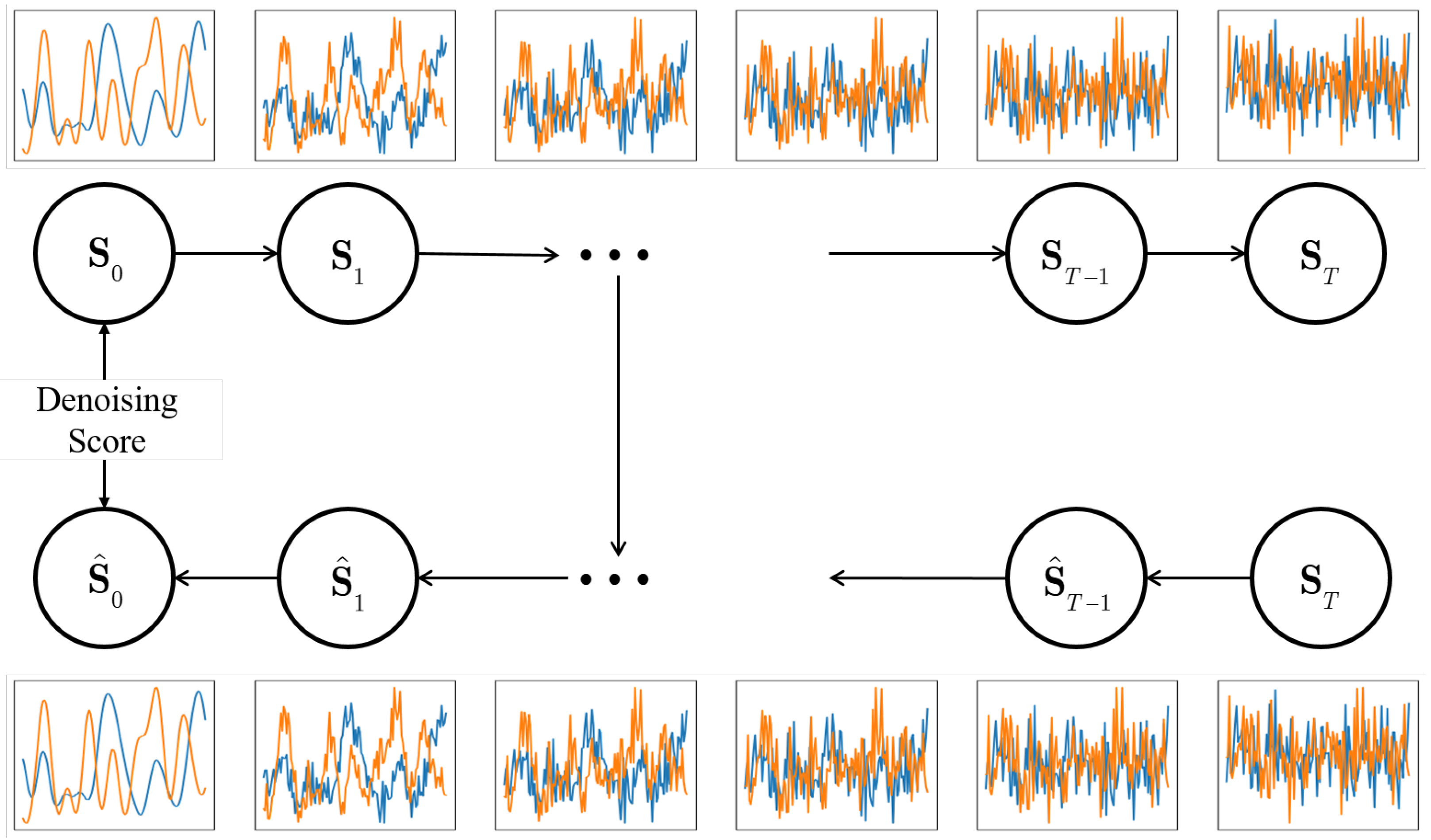
3.4. Denoising Score on Denoising Diffusion Model

The denoising diffusion model (DDM) [49,50] is a deep learning method that generates high-quality data samples by simulating a gradual noise removal process. Its core idea is derived from the diffusion process in statistical physics, particularly the transition from a high-entropy (disordered, high-noise) state to a low-entropy (ordered, low-noise) state. The DDM consists of two main components: the forward diffusion process and the reverse denoising process, as shown in Figure 2. The forward process is a Markov chain that progressively adds Gaussian noise to the data until it reaches a state that is close to a Gaussian distribution. The reverse process, in contrast, is a parameterized Markov chain in which a neural network is trained to determine how to remove noise from the noised data at each step, thereby gradually restoring the original data.
Due to its high quality and diversity in image generation, DDMs (denoising diffusion models) are gradually replacing GANs and becoming a key technology in various applications such as text-to-image generation [51], video generation [52], and speech synthesis [53]. DDMs have demonstrated strong capabilities in data generation, suggesting their ability to effectively capture data distributions, thereby providing an additional pathway for open-set recognition. All open-set recognition research based on DDMs in this paper was conducted using the DDIM framework provided by Mousai [54].

3.4.1. V -Objective Training

In the original denoising diffusion probabilistic model (DDPM) [49], during the reverse denoising process, the diffusion model is tasked with predicting the noise added at time step t 1 based on the noised s t at time step t. This prediction is implemented using an artificial neural network (ANN). As denoising diffusion models evolved, additional prediction objectives have been introduced alongside the noise prediction objective, such as the v -objective and the s ( 0 ) -objective. Essentially, training a DDM is about training an ANN so that it can accurately predict the desired objective. Since the prediction target of the ANN has the same shape as the input, most DDMs employ a U-Net architecture for the ANN. The DDM used for open-set recognition in this study utilizes UnetV0 provided by Mousai. For simplicity and to avoid the region devour issue mentioned in [55], we trained the diffusion model using data from a single KKC, resulting in the generation of C sets of model weights.
In Figure 2, the maximum diffusion step is set to T; then, for any time step t, the noised data s t can be obtained as
s ( σ t ) = α ( σ t ) · s 0 + β ( σ t ) · ϵ ,
α ( σ t ) = sin ( π 2 · σ t ) ,
β ( σ t ) = cos ( π 2 · σ t ) ,
σ t = t T ,
where ϵ is the noise sampled from a standard normal distribution N ( 0 , 1 ) , and σ t means the noise level. The v-objective is formulated as
v ( σ t ) = s ( σ t ) σ t = α ( σ t ) · ϵ β ( σ t ) · s 0 .
The intended meaning of v ( σ t ) is the noise-added velocity at a noise level of σ t . With noised data s t and noise level σ t as inputs, the v-objective-based DDM tries to estimate an ANN model
v ^ ( σ t ) = f u ( s ( σ t ) , σ t ) ,
where f u ( · , · ) denotes UNetV0 in this paper. The parameters in f u are optimized by minimizing the following function:
E t [ 0 , T ] | t Z , s σ t , σ t [ f u ( s ( σ t ) , σ t ) v ( σ t ) 2 2 ] .
In the training phase, the value of the maximum time step T is set very high, but the maximum value of σ t equals 1 however high T is. It should be noted that for every input s , its corresponding noise level σ t is randomly sampled from U [ 0 , 1 ] .

3.4.2. DDIM-Based Denoising Score

A well-trained DDM is capable of gradually denoising from pure noise to synthesize data that are consistent with the categories of the training samples. The core idea of using a DDM for OSR is to add noise of a fixed level to the input. For KKC samples, this noise can be effectively removed, whereas for UUC samples, the noise removal is less effective.
The first step in implementing OSR with a DDM involves adding a specific level of noise to the original input s ( 0 ) , as described in Equation (13). The noise level should be neither too small nor too large: a small noise level results in uniformly high noise removal, while a large noise level leads to uniformly low noise removal. In this study, the added noise level was set to 0.25, and the parameter T was set to 100. The value of T during inference can differ from its value during training, as the noise level’s maximum value remains 1 regardless of the value of T. The second step involves denoising the input using the DDIM algorithm with f u , s ( σ t ) , σ t following the following specific steps:
  • Input s ( σ t ) and σ t into f u to produce an estimate of the velocity as
    v ^ ( σ t ) = f u ( s ( σ t ) , σ t ) .
  • Calculate an estimation of s at time step 0 based on Equations (13) and (17) as
    s ^ ( 0 ) = α ( σ t ) · s ( σ t ) β ( σ t ) · v ^ ( σ t ) .
  • Calculate a noise estimation of ϵ at noise level σ t based on Equations (13) and (17) as
    ϵ ^ ( σ t ) = β ( σ t ) · s ( σ t ) + α ( σ t ) · v ^ ( σ t ) .
  • Calculate an estimation for s at time step t 1 as
    s ^ ( σ t 1 ) = α ( σ t 1 ) · s ^ ( 0 ) + β ( σ t 1 ) · ϵ ^ ( σ t ) .
As shown in the above equations, the maximum value of t equals 25 as we set T = 100 and noise levels { σ 0 = 0.0 , σ 1 = 0.01 , , σ 25 = 0.25 } are pre-scheduled.
The above denoising steps should be repeated until t = 0 , which is shown in Figure 2. After the denoising procedure, a quantized score is required for OSR; thus, we designed the denoising score using the original input s 0 and its estimation s ^ 0 , which is formulated as
S d d m ( s ( 0 ) ; f u ) = exp ( s ( 0 ) s ^ ( 0 ) 2 2 )

3.5. Class-Wise Threshold Co-Calibration

The primary motivation for incorporating the DDM is to utilize instance-level denoising scores to further refine the close prediction results along with CPL scores, which are class-level. The introduction of denoising scores is excepted to bring more criteria.
In this paper, we treat an OSAMR task with C KKCs as C binary classification tasks, with the following steps.
For a given unlabeled testing sample s , calculate its CPL logits and subsequently obtain its predicted label y ^ with the following equation:
L o g i t c p l ( s , P k ; f θ ) = 1 | CosineSim ( f θ ( s ) , P k ) R | ,
y ^ = arg max k { L o g i t c p l ( s , P k ; f θ ) } k = 1 C ,
where the value of L o g i t c p l ( s , P k ; f θ ) is limited to [ 1 , 1 ] . Now that the predicted label y ^ is available, the denoising score of s can be obtained through Equation (24). It should be noted that the parameters of f u are instantiated with those trained using samples of class y ^ . The next step is to calculate the integrated score:
S ( s ; P , f θ , f u , y ^ ) = λ · L o g i t c p l ( s , P y ^ ; f θ ) + ( 1 λ ) · S d d m ( s ; f u y ^ ) ,
where f u y ^ denotes UNetV0 trained with samples of class y ^ , and the hyper-parameter λ is adopted to balance the two components. The magnitudes of the two scores are consistent, and they can be directly added together. Additionally, a threshold is required for class y ^ , denoted as t h y ^ , with which calibration on the close-set prediction y ^ can be achieved as
y = y ^ S ( s ; P , f θ , f u , y ^ ) t h y ^ , C + 1 else .
A crucial aspect of this process is that the close prediction result is produced using CPL, while the DDM does not possess classification capabilities. Open-set recognition can be accomplished using only CPL; however, it cannot be achieved using only a DDM, as the DDM relies on the close prediction results generated via CPL.
The threshold for each KKC can be obtained manually or statistically. As for determining a threshold for a class by statistical methods, one general approach is to select a threshold based on the scores of training samples that can cover δ of those samples as known, where δ [ 0 , 1 ] . The threshold determination process for class k under the δ condition is formulated in
t h k = min t h { p [ S ( s ; P , f θ , f u , k ) > t h | t h R ] δ } .
Determining a threshold for each KKC does not introduce significant time complexity, as the threshold for a single KKC is determined using only the training samples of that class without involving samples from other classes. In other words, each sample is used only once, which is consistent with determining a shared threshold for all KKCs.

4. Results

4.1. Datasets

To evaluate the effectiveness of the proposed CPLDiff framework in the OSAMR task, we conducted comparative experiments on two publicly available modulation signal datasets: RadioML2016.10a and RadioML2016.04c [56]. A concise description and the OSAMR task settings are provided in Table 2.

4.2. Experimental Setup

4.2.1. Environment

All experiments were implemented using PyTorch 1.12.1 and conducted on a computer with an Intel (R) 12600KF CPU with 128 GB of RAM and an NVIDIA RTX 3090 GPU with 24 GB of RAM.

4.2.2. Parameters and Models

In the following experiments, we set τ = 0.05 and R = 0.2 in Equation (11). The AdamW [57] optimizer was used for updating f θ and f u , the learning rate was set to 0.001 for both the training of the CPL and DDM, the batch size was 640, and the total numbers of training epochs were 300 for CPL and 400 for DDM. For prototype pre-optimization, the number of training epochs was 20,000. In the denoising score calculation procedure, T was set to 100, and noise level σ was set to 0.25. The hyper-parameter λ in Equation (27) was set to 0.8. The modulated signal encoder was SigRes34 in [38].

4.2.3. Evaluation Metrics

There are three commonly used evaluation metrics for OSR tasks, including the area under the receiver operating characteristic (AUROC) curve, Open-Set Classification Rate (OSCR), and True Negative Rate (TNR).
  • AUROC. The receiver operating characteristic (ROC) curve is used to evaluate the prediction performance of a binary classification model. This is achieved by plotting the model’s True Positive Rate (TPR) against the False Positive Rate (FPR) at various threshold settings, resulting in a curve that describes the classification model’s performance. The AUROC refers to the area under the ROC curve, which is commonly used to quantify the overall performance of a binary classification model. Its value ranges from 0 to 1, with larger values indicating better classification performance.
  • OSCR. This metric improves the AUROC by replacing the TPR value with the Correct Classification Rate (CCR) while keeping the same FPR. In this manner, the OSCR takes into accounts the classification performance of the OSR algorithm. The value of the OSCR also ranges from 0 to 1 and is commonly lower than the value of the AUROC for declines in classification accuracy.
  • TNR. This metric indicates the detection rate for UUC samples. As the goal of the OSR is to detect UUC samples while remaining high in KKC recognition accuracy, the TNR is generally obtained under the condition that the TPR equals 95%.

4.3. Experimental Results

To evaluate the effectiveness of the proposed CPLDiff framework in the OSAMR task, we simulated open-set modulation recognition scenarios using two publicly available modulation signal datasets, RadioML2016.10a and RadioML2016.04c, with specific settings detailed in Table 2. Unless otherwise specified, all experimental figures and charts in this subsection are based on relatively clean data, specifically data with Signal-to-Noise Ratios (SNRs) of 12, 14, 16, and 18 dB. The OSAMR experimental results of CPLDiff were compared against those of the SoftMax baseline method [42], GCPL [16], ARPL [15], and ARPL+CS [15]. To ensure fairness in comparison, identical data processing methods and feature extractors were applied across all approaches.

4.3.1. OSAMR Performance

Table 3 and Table 4 present the AUROC, OSCR, and TNR results for the RadioML2016.10a and RadioML2016.04c datasets. The results indicate that the proposed CPLDiff method achieves the highest values across all the quantitative metrics, demonstrating superior OSR performance compared to the other methods. Specifically, as shown in rows 0 to 8 of Table 3 for class-wise AUROC values, the SoftMax baseline method exhibits a relatively low value for Class QAM16, suggesting that the UUCs are prone to confusion with this class. Moreover, the GCPL method also shows a lower AUROC value for Class QPSK compared to other classes, and a similar phenomenon is observed in the ARPL and ARPL+CS methods. Therefore, the AUROC values across different classes reveal that the comparison methods tend to confuse the UUCs with certain KKC(s). In contrast, for the CPLDiff method, the class-wise AUROC values in Table 3 remain consistently high, with the AUROC values for Class QAM16 and Class QPSK exceeding 98. A similar phenomenon can be observed in Table 4.
Figure 3 shows the ROC and OSCR curves obtained from open-set experiments on the 10a and 04c datasets. The ROC curve was generated by gradually increasing the threshold, resulting in a series of (TPR, TNR) pairs, and the OSCR curve is generated in a similar manner. The results in the figures demonstrate that the CPLDiff method achieves the best OSAMR performance. Specifically, for the CPLDiff method, it rapidly increases the TPR and CCR while maintaining a low FPR. In contrast, for the other methods, as the TPR and CCR increase, the FPR also rises at a certain rate, failing to maintain a low FPR at higher TPR levels.

4.3.2. Recognition on KKC and Detection on UUC

The goal of OSAMR is to ensure the recognition performance on KKCs while maximizing the detection capability for UUCs. As described in Section 3.1, the open-set recognition task can be viewed as a C + 1 classification task, where all UUCs are treated as a single class. To specifically and clearly demonstrate the performance of the proposed CPLDiff algorithm in terms of recognition on KKCs and detection on UUCs, we present the TNR data, as well as the prediction confusion matrix for the C + 1 classification task.
Table 3 and Table 4 present the detection rates for UUCs using the proposed CPLDiff algorithm on the 10a and 04c datasets, as shown in the TNR row. It is evident from the table that the proposed algorithm achieves the highest TNR values. Specifically, for the 10a dataset, the detection rate for the unknown class is 96.95%, which is over a 20% improvement compared to the second-highest GCPL algorithm at 75.12%.
Figure 4 provides a more detailed view through the confusion matrices for the OSAMR tasks from the CPLDiff, GCPL, and SoftMax algorithms, clearly illustrating the confusions between KKC and KKC, as well as between KKC and UUC. The conditions for generating these confusion matrices are outlined in the table notes of Table 3. In the confusion matrices, the true labels for KKCs and UUCs are provided, where the predicted labels include “Unknown” in addition to the KKC labels. From the displayed matrices, it is clear that there is no significant confusion between KKC and UUC for CPLDiff. The proposed algorithm maintains a high recognition rate for KKC while also achieving a high detection rate for UUC. In contrast, GCPL struggles to distinguish between QAM16 and QAM64, two KKCs, and exhibits considerable confusion between UUCs and the QPSK modulation scheme in the RadioML2016.10a dataset. The SoftMax baseline method performs best in KKC recognition but has the poorest detection rate for UUCs.

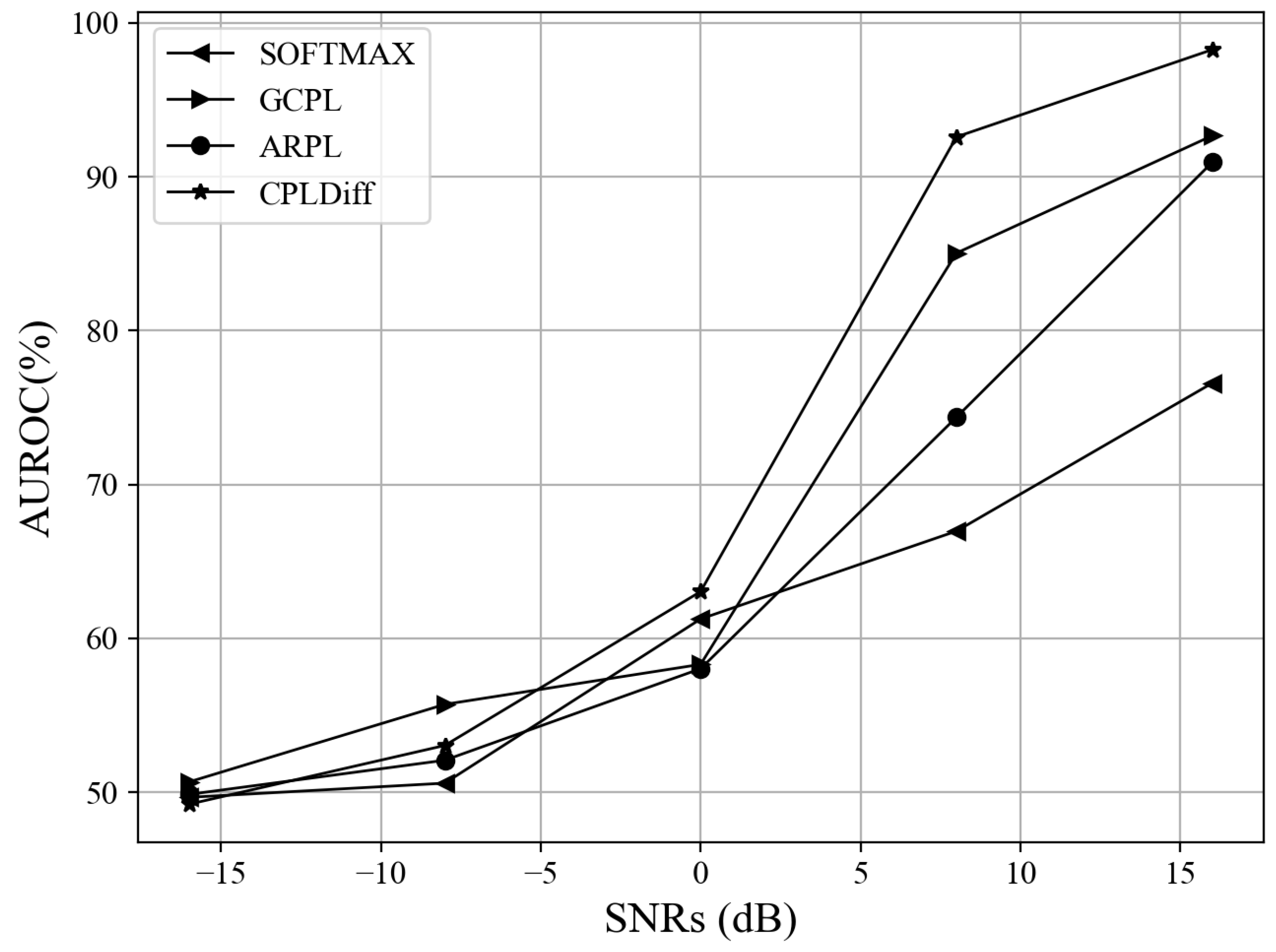
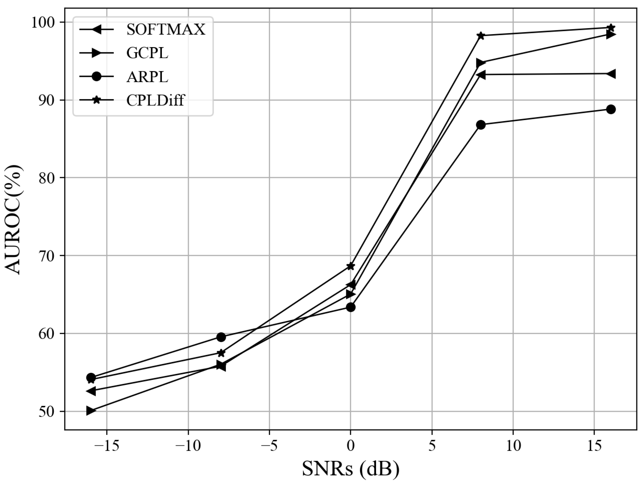
4.3.3. OSAMR Results at Different SNRs

Due to the impact of noise on signals in real-world environments, we conducted experiments at different SNR levels. For the 10a and 04c datasets, we divided the SNR (dB) into five levels—{−20, −18, −16, −14}, {−12, −10, −8, −6}, {−4, −2, 0, 2}, {4, 6, 8, 10}, and {12, 14, 16, 18}—and conducted experiments using data at each of these noise levels. The experimental results are shown in Figure 5 and Figure 6.
From the experimental results, three conclusions can be drawn. First, under low-SNR (dB) conditions of [−20, −6], the AUROC performance of all methods is close to 50%, meaning that they cannot distinguish between KKCs and UUCs. In such low-SNR conditions, the energy of the noise far exceeds that of the signal, causing the signal’s meaningful features to be masked by the noise. This results in a high level of randomness in the algorithm’s performance, and small differences may not accurately reflect the superiority of one algorithm over another.
Second, as the SNR increases, the AUROC performance of all algorithms shows an upward trend. Among them, the proposed algorithm exhibits the largest improvement, which also indirectly suggests that noise has a significant impact on the DDM. Since the DDM aims to restore pure original data, the introduction of noise can significantly interfere with the denoising process in the DDM.
Third, at higher SNR levels, the AUROC performance of the proposed method outperforms the other algorithms. In real-world environments, the SNR (dB) typically falls within the range of [10, 30], indicating that the proposed algorithm is more suitable for application in practical scenarios.

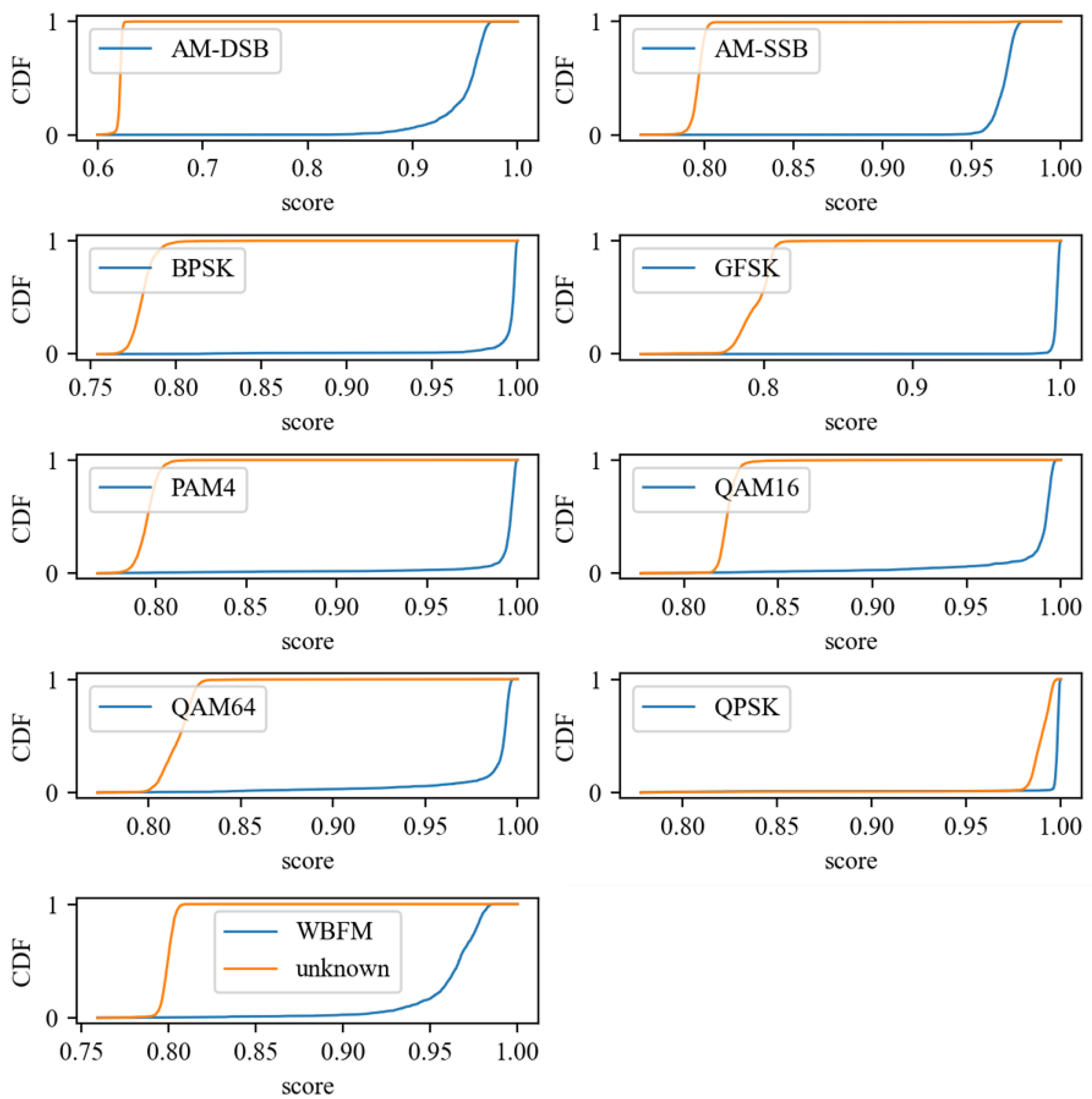
4.3.4. Visualization

In this subsection, we present the cumulative distribution function (CDF) of the test sample scores in Figure 7, which helps to better understand the distribution of sample scores. From the cumulative distribution function of the scores, it can be observed that the scores of KKC samples are mostly concentrated in the range [0.95, 1], while the scores of UUC samples are generally lower than those of the KKC samples.
Many methods define the open-set recognition task as a binary classification problem and assign a score to each sample. In this open-set recognition paradigm, all known known classes (KKCs) share the same threshold. The approach of using a single threshold for all KKCs is effective under the condition that the score distributions of all KKCs are consistent. However, as shown in Figure 7, the score distributions are inconsistent due to variations in the data across different categories, making the use of a shared threshold severely flawed. Therefore, it is essential to determine thresholds individually for each KKC. This does not introduce significant time complexity, as the threshold for a single KKC is determined using only the training samples of that class without involving samples from other classes. In other words, each sample is used only once, which is consistent with determining a shared threshold for all KKCs.

4.4. Further Experiments

4.4.1. Effectiveness of DDM

The primary motivation for incorporating a DDM is to utilize instance-level denoising scores to further refine the close prediction results along with CPL scores. Therefore, in this context, we compare the results of performing open-set recognition using only CPL with those achieved using CPLDiff (the combination of CPL and DDM) to validate the effectiveness of introducing the DDM in Table 5. It is evident that CPL already exhibits a certain level of open-set recognition capability. Upon incorporating the denoising scores generated by the DDM, the open-set recognition metrics for both datasets showed varying degrees of improvement. This indicates that the instance-level information enhanced by the DDM contributes to the effectiveness of open-set recognition.

4.4.2. Few-Shot Performance

We further conducted experiments in few-shot scenarios, as the DDM is capable of generating synthetic samples for data augmentation. For instance, Chen et al. [58] employed a conditional diffusion model to generate synthetic data to assist the model in few-shot cases and proved its effectiveness. Following their work, we evaluated the data augmentation effectiveness of the DDM in both close-set AMR and open-set AMR tasks.
Specifically, we limited the available training data to 5% samples per class and augmented the training dataset with additional 2000 synthetic samples per class generated by the conditional diffusion model. Notably, the conditional diffusion model was consistently trained with the limited 5% samples. We selected one synthetic sample for each class and visualized the data in terms of waveforms and constellation diagrams in Figure 8.
For few-shot close-set AMR tasks, we compared the classification performance of Softmax, GCPL, ARPL, ARPL+CS, CPL and CPL+, where CPL+ means the CPL trained jointly with the original and synthetic samples. The results are shown in Table 6, where the precision, recall, and F1 score are commonly used metrics in classification tasks, and recall refers to the accuracy. From the table, we can draw the following conclusions. First, compared to 70% training samples, limited available data introduces a decline in the AMR performance for all methods. Second, SoftMax achieves the best recognition performance among the comparison methods, and CPL is competitive against SoftMax, exhibiting more robustness in few-shot scenarios. Finally, CPL+, which shows improvements from CPL, demonstrated the effectiveness of the data augmentation strategy with the DDM.
For few-shot open-set AMR, we compared the three OSR metric results in Table 7, where CPLDiff+ means training the CPL module with additional synthetic samples. It is obvious that all the methods suffered declines in terms of the three OSR metrics, which indicates that the insufficiency of training data poses great challenges for the methods to learn competitive encoders and classifiers. While the comparison methods suffer significant performance declines, CPLDiff shows more robustness in such few-shot scenarios, and CPLDiff+ further enhances performance from that of CPLDiff. The CPL adopts data-free pre-prototype optimization before training the encoder, which provides CPL with more robust prototype retrievals. Additionally, the DDM is UNet-enabled, which brings more adaptivity to few-shot scenarios.

5. Conclusions

In this paper, the CPLDiff method is proposed to achieve open-set automatic modulation recognition, requiring a detection ability over unknown classes. We analyze the shortcomings of existing OSR methods and demonstrate the main challenge that CPLDiff is to solve. In order to fully exploit and leverage the training samples of known known classes, we combine CPL and a DDM, with the former extracting class-level information and the latter extracting instance-level information.
To demonstrate the OSAMR effectiveness of CPLDiff, we conducted several comparative experiments on the public datasets RadioML2016.10a and RadioML2016.04c. Experimental results show that the CPLDiff algorithm outperforms other state-of-the-art methods with respect to the AUROC, OSCR, and TNR metrics, even when the unknown unknown classes share great similarity with some of the known known classes. The OSAMR results at different SNRs indicate that our method is suitable for real-world environments. We further evaluate the robustness of CPLDiff in resource-constrained settings. However, there exist several limitations in the CPLDiff algorithm. First, due to the co-inference and denoising loop in the DDM, CPLDiff is time-consuming compared to other methods. Second, a large scale of training samples is required to fully leverage the DDM. In future research, the OSR paradigms with a DDM need more exploration except for with the proposed denoising score, such as by developing a lightweight DDM and data augmentation strategy.

Author Contributions

Methodology development, H.N.; data collection, experiment conduction, and result analysis, H.N. and X.X.; writing—original draft, X.C.; writing—review and editing, X.C. and J.B. All authors have read and agreed to the published version of the manuscript.

Funding

This work was supported in part by the National Natural Science Foundation of China under Grant 62276206, in part by the Aeronautical Science Foundation of China under Grant 2023Z071081001.

Data Availability Statement

The original data presented in the study are openly available at https://www.deepsig.ai/datasets (accessed on 24 March 2023).

Conflicts of Interest

The authors declare no conflict of interest.

References

  1. Peng, S.; Sun, S.; Yao, Y.D. A survey of modulation classification using deep learning: Signal representation and data preprocessing. IEEE Trans. Neural Netw. Learn. Syst. 2021, 33, 7020–7038. [Google Scholar] [CrossRef] [PubMed]
  2. Kulin, M.; Kazaz, T.; Moerman, I.; De Poorter, E. End-to-End Learning From Spectrum Data: A Deep Learning Approach for Wireless Signal Identification in Spectrum Monitoring Applications. IEEE Access 2018, 6, 18484–18501. [Google Scholar] [CrossRef]
  3. Di, C.; Ji, J.; Sun, C.; Liang, L. SOAMC: A Semi-Supervised Open-Set Recognition Algorithm for Automatic Modulation Classification. Electronics 2024, 13, 4196. [Google Scholar] [CrossRef]
  4. Zheng, S.; Chen, S.; Yang, L.; Zhu, J.; Luo, Z.; Hu, J.; Yang, X. Big data processing architecture for radio signals empowered by deep learning: Concept, experiment, applications and challenges. IEEE Access 2018, 6, 55907–55922. [Google Scholar] [CrossRef]
  5. Wang, H.; Liu, Z.; Wang, X.; Meng, X.; Wu, Y.; Han, Z. Model-Based Data-Efficient Reinforcement Learning for Active Pantograph Control in High-Speed Railways. IEEE Trans. Transp. Electrif. 2024, 10, 2701–2712. [Google Scholar] [CrossRef]
  6. Meng, X.; Hu, G.; Liu, Z.; Wang, H.; Zhang, G.; Lin, H.; Sadabadi, M.S. Neural Network-Based Impedance Identification and Stability Analysis for Double-Sided Feeding Railway Systems. IEEE Trans. Transp. Electrif. 2024; early access. [Google Scholar] [CrossRef]
  7. Scheirer, W.J.; de Rezende Rocha, A.; Sapkota, A.; Boult, T.E. Toward open set recognition. IEEE Trans. Pattern Anal. Mach. Intell. 2012, 35, 1757–1772. [Google Scholar] [CrossRef] [PubMed]
  8. Li, T.; Wen, Z.; Long, Y.; Hong, Z.; Zheng, S.; Yu, L.; Chen, B.; Yang, X.; Shao, L. The importance of expert knowledge for automatic modulation open set recognition. IEEE Trans. Pattern Anal. Mach. Intell. 2023, 45, 13730–13748. [Google Scholar] [CrossRef] [PubMed]
  9. Hu, G.; Meng, X.; Wang, X.; Liu, Z. A Novel Explainable Impedance Identification Method Based on Deep Learning for the Vehicle-grid System of High-speed Railways. IEEE Trans. Transp. Electrif. 2024; early access. [Google Scholar] [CrossRef]
  10. Meng, X.; Zhang, Q.; Liu, Z.; Hu, G.; Liu, F.; Zhang, G. Multiple Vehicles and Traction Network Interaction System Stability Analysis and Oscillation Responsibility Identification. IEEE Trans. Power Electron. 2024, 39, 6148–6162. [Google Scholar] [CrossRef]
  11. Pimentel, M.A.; Clifton, D.A.; Clifton, L.; Tarassenko, L. A review of novelty detection. Signal Process. 2014, 99, 215–249. [Google Scholar] [CrossRef]
  12. Zhou, H.; Bai, J.; Niu, L.; Xu, J.; Xiao, Z.; Zheng, S.; Jiao, L.; Yang, X. Electromagnetic signal classification based on class exemplar selection and multi-objective linear programming. Remote Sens. 2022, 14, 1177. [Google Scholar] [CrossRef]
  13. Masana, M.; Liu, X.; Twardowski, B.; Menta, M.; Bagdanov, A.D.; Van De Weijer, J. Class-incremental learning: Survey and performance evaluation on image classification. IEEE Trans. Pattern Anal. Mach. Intell. 2022, 45, 5513–5533. [Google Scholar] [CrossRef]
  14. Salehi, M.; Mirzaei, H.; Hendrycks, D.; Li, Y.; Rohban, M.H.; Sabokrou, M. A unified survey on anomaly, novelty, open-set, and out-of-distribution detection: Solutions and future challenges. arXiv 2021, arXiv:2110.14051. [Google Scholar]
  15. Chen, G.; Peng, P.; Wang, X.; Tian, Y. Adversarial reciprocal points learning for open set recognition. IEEE Trans. Pattern Anal. Mach. Intell. 2021, 44, 8065–8081. [Google Scholar] [CrossRef]
  16. Yang, H.M.; Zhang, X.Y.; Yin, F.; Liu, C.L. Robust classification with convolutional prototype learning. In Proceedings of the IEEE Conference on Computer Vision and Pattern Recognition, Salt Lake City, UT, USA, 19–21 June 2018; pp. 3474–3482. [Google Scholar]
  17. Goodfellow, I.; Pouget-Abadie, J.; Mirza, M.; Xu, B.; Warde-Farley, D.; Ozair, S.; Courville, A.; Bengio, Y. Generative adversarial nets. Adv. Neural Inf. Process. Syst. 2014, 27. [Google Scholar] [CrossRef]
  18. Oza, P.; Patel, V.M. C2ae: Class conditioned auto-encoder for open-set recognition. In Proceedings of the IEEE/CVF Conference on Computer Vision and Pattern Recognition, Long Beach, CA, USA, 18–20 June 2019; pp. 2307–2316. [Google Scholar]
  19. Yoshihashi, R.; Shao, W.; Kawakami, R.; You, S.; Iida, M.; Naemura, T. Classification-reconstruction learning for open-set recognition. In Proceedings of the IEEE/CVF Conference on Computer Vision and Pattern Recognition, Long Beach, CA, USA, 18–20 June 2019; pp. 4016–4025. [Google Scholar]
  20. Tishby, N.; Zaslavsky, N. Deep learning and the information bottleneck principle. In Proceedings of the 2015 IEEE Information Theory Workshop (ITW), Jerusalem, Israel, 26 April–1 May 2015; pp. 1–5. [Google Scholar]
  21. Huan, C.Y.; Polydoros, A. Likelihood methods for MPSK modulation classification. IEEE Trans. Commun. 1995, 43, 1493–1504. [Google Scholar] [CrossRef]
  22. Wang, L.X.; Ren, Y.J. Recognition of digital modulation signals based on high order cumulants and support vector machines. In Proceedings of the 2009 ISECS International Colloquium on Computing, Communication, Control, and Management, Sanya, China, 8–9 August 2009; Volume 4, pp. 271–274. [Google Scholar]
  23. Das, D.; Bora, P.K.; Bhattacharjee, R. Cumulant based automatic modulation classification of QPSK, OQPSK, 8-PSK and 16-PSK. In Proceedings of the 2016 8th International Conference on Communication Systems and Networks (COMSNETS), Bangalore, India, 5–10 January 2016; pp. 1–5. [Google Scholar]
  24. Xie, L.; Wan, Q. Cyclic feature-based modulation recognition using compressive sensing. IEEE Wirel. Commun. Lett. 2017, 6, 402–405. [Google Scholar] [CrossRef]
  25. O’Shea, T.J.; Roy, T.; Clancy, T.C. Over-the-air deep learning based radio signal classification. IEEE J. Sel. Top. Signal Process. 2018, 12, 168–179. [Google Scholar] [CrossRef]
  26. Chen, Z.; Cui, H.; Xiang, J.; Qiu, K.; Huang, L.; Zheng, S.; Chen, S.; Xuan, Q.; Yang, X. SigNet: A Novel Deep Learning Framework for Radio Signal Classification. IEEE Trans. Cogn. Commun. Netw. 2022, 8, 529–541. [Google Scholar] [CrossRef]
  27. Liu, X.; Yang, D.; El Gamal, A. Deep neural network architectures for modulation classification. In Proceedings of the 2017 51st Asilomar Conference on Signals, Systems, and Computers, Pacific Grove, CA, USA, 29 October–1 November 2017; pp. 915–919. [Google Scholar]
  28. Zhu, H.; Ma, Y.; Zhang, X.; Hao, C. Adaptive Denoising With Efficient Channel Attention for Automatic Modulation Recognition. In Proceedings of the ICC 2024-IEEE International Conference on Communications, Denver, CO, USA, 9–13 June 2024; pp. 2113–2118. [Google Scholar]
  29. Chen, J.; Teo, T.H.; Kok, C.L.; Koh, Y.Y. A Novel Single-Word Speech Recognition on Embedded Systems Using a Convolution Neuron Network with Improved Out-of-Distribution Detection. Electronics 2024, 13, 530. [Google Scholar] [CrossRef]
  30. Wang, Y.; Bai, J.; Xiao, Z.; Zhou, H.; Jiao, L. MsmcNet: A Modular Few-Shot Learning Framework for Signal Modulation Classification. IEEE Trans. Signal Process. 2022, 70, 3789–3801. [Google Scholar] [CrossRef]
  31. Chen, Y.; Shao, W.; Liu, J.; Yu, L.; Qian, Z. Automatic modulation classification scheme based on LSTM with random erasing and attention mechanism. IEEE Access 2020, 8, 154290–154300. [Google Scholar] [CrossRef]
  32. Hamidi-Rad, S.; Jain, S. Mcformer: A transformer based deep neural network for automatic modulation classification. In Proceedings of the 2021 IEEE Global Communications Conference (GLOBECOM), Madrid, Spain, 7–11 December 2021; pp. 1–6. [Google Scholar]
  33. Lei, J.; Li, Y.; Yung, L.Y.; Leng, Y.; Lin, Q.; Wu, Y.C. Understanding Complex-Valued Transformer for Modulation Recognition. IEEE Wirel. Commun. Lett. 2024, 13, 3523–3527. [Google Scholar] [CrossRef]
  34. Xu, J.; Luo, C.; Parr, G.; Luo, Y. A Spatiotemporal Multi-Channel Learning Framework for Automatic Modulation Recognition. IEEE Wirel. Commun. Lett. 2020, 9, 1629–1632. [Google Scholar] [CrossRef]
  35. Zhang, Z.; Luo, H.; Wang, C.; Gan, C.; Xiang, Y. Automatic modulation classification using CNN-LSTM based dual-stream structure. IEEE Trans. Veh. Technol. 2020, 69, 13521–13531. [Google Scholar] [CrossRef]
  36. Ruikar, J.D.; Park, D.H.; Kwon, S.Y.; Kim, H.N. HCTC: Hybrid Convolutional Transformer Classifier for Automatic Modulation Recognition. Electronics 2024, 13, 3969. [Google Scholar] [CrossRef]
  37. Deng, W.; Wang, X.; Huang, Z.; Xu, Q. Modulation Classifier: A Few-Shot Learning Semi-Supervised Method Based on Multimodal Information and Domain Adversarial Network. IEEE Commun. Lett. 2023, 27, 576–580. [Google Scholar] [CrossRef]
  38. Bai, J.; Wang, X.; Xiao, Z.; Zhou, H.; Ali, T.A.A.; Li, Y.; Jiao, L. Achieving efficient feature representation for modulation signal: A cooperative contrast learning approach. IEEE Internet Things J. 2024, 11, 16196–16211. [Google Scholar] [CrossRef]
  39. Bai, J.; Liu, X.; Wang, Y.; Xiao, Z.; Chen, F.; Zhou, H.; Jiao, L. Integrating Prior Knowledge and Contrast Feature for Signal Modulation Classification. IEEE Internet Things J. 2024, 11, 21461–21473. [Google Scholar] [CrossRef]
  40. Rajendran, S.; Meert, W.; Giustiniano, D.; Lenders, V.; Pollin, S. Deep learning models for wireless signal classification with distributed low-cost spectrum sensors. IEEE Trans. Cogn. Commun. Netw. 2018, 4, 433–445. [Google Scholar] [CrossRef]
  41. Geng, C.; Huang, S.j.; Chen, S. Recent advances in open set recognition: A survey. IEEE Trans. Pattern Anal. Mach. Intell. 2020, 43, 3614–3631. [Google Scholar] [CrossRef] [PubMed]
  42. Hendrycks, D.; Gimpel, K. A baseline for detecting misclassified and out-of-distribution examples in neural networks. arXiv 2016, arXiv:1610.02136. [Google Scholar]
  43. Bendale, A.; Boult, T.E. Towards open set deep networks. In Proceedings of the IEEE Conference on Computer Vision and Pattern Recognition (CVPR), Las Vegas, NV, USA, 26 June–1 July 2016; pp. 1563–1572. [Google Scholar]
  44. Zhou, D.W.; Ye, H.J.; Zhan, D.C. Learning placeholders for open-set recognition. In Proceedings of the IEEE/CVF Conference on Computer Vision and Pattern Recognition (CVPR), Virtual, 21–25 June 2021; pp. 4401–4410. [Google Scholar]
  45. Chen, G.; Qiao, L.; Shi, Y.; Peng, P.; Li, J.; Huang, T.; Pu, S.; Tian, Y. Learning open set network with discriminative reciprocal points. In Proceedings of the Computer Vision–ECCV 2020: 16th European Conference, Glasgow, UK, 23–28 August 2020; Proceedings, Part III 16. Springer: Berlin/Heidelberg, Germany, 2020; pp. 507–522. [Google Scholar]
  46. Ge, Z.; Demyanov, S.; Chen, Z.; Garnavi, R. Generative openmax for multi-class open set classification. arXiv 2017, arXiv:1707.07418. [Google Scholar]
  47. Neal, L.; Olson, M.; Fern, X.; Wong, W.K.; Li, F. Open set learning with counterfactual images. In Proceedings of the European Conference on Computer Vision (ECCV), Munich, Germany, 8–14 September 2018; pp. 613–628. [Google Scholar]
  48. Shah, S.A.W.; Abed-Meraim, K.; Al-Naffouri, T.Y. Multi-modulus algorithms using hyperbolic and Givens rotations for blind deconvolution of MIMO systems. In Proceedings of the 2015 IEEE International Conference on Acoustics, Speech and Signal Processing (ICASSP), South Brisbane, Australia, 19–24 April 2015; pp. 2155–2159. [Google Scholar]
  49. Ho, J.; Jain, A.; Abbeel, P. Denoising diffusion probabilistic models. Adv. Neural Inf. Process. Syst. 2020, 33, 6840–6851. [Google Scholar]
  50. Song, J.; Meng, C.; Ermon, S. Denoising diffusion implicit models. arXiv 2020, arXiv:2010.02502. [Google Scholar]
  51. Qiao, T.; Zhang, J.; Xu, D.; Tao, D. Mirrorgan: Learning text-to-image generation by redescription. In Proceedings of the IEEE/CVF Conference on Computer Vision and Pattern Recognition (CVPR), Long Beach, CA, USA, 18–20 June 2019; pp. 1505–1514. [Google Scholar]
  52. Ho, J.; Chan, W.; Saharia, C.; Whang, J.; Gao, R.; Gritsenko, A.; Kingma, D.P.; Poole, B.; Norouzi, M.; Fleet, D.J.; et al. Imagen video: High definition video generation with diffusion models. arXiv 2022, arXiv:2210.02303. [Google Scholar]
  53. Zhang, C.; Zhang, C.; Zheng, S.; Zhang, M.; Qamar, M.; Bae, S.H.; Kweon, I.S. A survey on audio diffusion models: Text to speech synthesis and enhancement in generative ai. arXiv 2023, arXiv:2303.13336. [Google Scholar]
  54. Schneider, F.; Kamal, O.; Jin, Z.; Schölkopf, B. Moûsai: Efficient text-to-music diffusion models. In Proceedings of the 62nd Annual Meeting of the Association for Computational Linguistics (Volume 1: Long Papers), Bangkok, Thailand, 11–16 August 2024; pp. 8050–8068. [Google Scholar]
  55. Huang, H.; Wang, Y.; Hu, Q.; Cheng, M.M. Class-specific semantic reconstruction for open set recognition. IEEE Trans. Pattern Anal. Mach. Intell. 2022, 45, 4214–4228. [Google Scholar] [CrossRef]
  56. O’Shea, T.J.; Corgan, J.; Clancy, T.C. Convolutional radio modulation recognition networks. In Proceedings of the Engineering Applications of Neural Networks: 17th International Conference, EANN 2016, Aberdeen, UK, 2–5 September 2016; Proceedings 17. Springer: Berlin/Heidelberg, Germany, 2016; pp. 213–226. [Google Scholar]
  57. Loshchilov, I. Decoupled weight decay regularization. arXiv 2017, arXiv:1711.05101. [Google Scholar]
  58. Chen, J.; Zhao, C.; Huang, X.; Wu, Z. Data Augmentation Aided Automatic Modulation Recognition Using Diffusion Model. In Proceedings of the 2024 IEEE Wireless Communications and Networking Conference (WCNC), Dubai, United Arab Emirates, 21–24 April 2024; pp. 1–6. [Google Scholar]
Figure 1. OSAMR workflow for a 3-classification task based on CPLDiff. First, CPL outputs the close-set prediction and the corresponding score. Second, a noise of a certain level is added to the input, and a DDIM is used to quantize the denoising score. Finally, the two scores are weight-summed, and the overall integrated score is used for calibration on the close-set prediction.
Electronics 14 00430 g001
Figure 2. The denoising score calculation procedure of a modulated signal where the orange and blue waveforms are the I and Q channel respectively. We set T to 100 and add noise of level 0.25 to the original input s 0 . Then, the noise is gradually removed using the DDIM algorithm. We quantize the noise removal as the denoising score.
Electronics 14 00430 g002
Figure 3. ROC curves and OSCR curves for the 10a and 04c datasets.
Electronics 14 00430 g003
Figure 4. Confusion matrix of OSAMR results.
Electronics 14 00430 g004aElectronics 14 00430 g004b
Figure 5. AUROC performance at different SNRs for RadioML2016.10a.
Electronics 14 00430 g005
Figure 6. AUROC performance at different SNRs for RadioML2016.04c.
Electronics 14 00430 g006
Figure 7. Cumulative distribution function (CDF) over score for each KKC in RadioML2016.10a.
Electronics 14 00430 g007
Figure 8. Waveform and constellation visualization of synthetic signals from DDM trained on 5% samples of RML2016.10a.
Electronics 14 00430 g008
Table 1. Difference between close-set AMR and open-set AMR.
TaskTrainingTestingGoal
Close-set AMRKKCsKKCsclassifying KKCs
Open-set AMRKKCsKKCs and UUCsidentifying KKCs and rejecting UUCs
Table 2. Dataset description and OSAMR task settings.
ItemsRadioML2016.10aRadioML2016.04c
Max carrier frequency offset50 Hz100 Hz
Max sampling rate offset500 Hz1000 Hz
Energy normalizationYesNo
Number of modulation schemes1111
Signal shape 2 × 128 2 × 128
SNR range (dB)−20∼18, with an interval of 2−20∼18, with an interval of 2
Number of signals per SNR11,0008103
Number of sinusoids used in frequency selective fading88
Channel environmentAdditive Gaussian white noise, selective fading (Rician + Rayleigh), Center Frequency Offset (CFO), Sample Rate Offset (SRO)Additive Gaussian white noise, selective fading (Rician + Rayleigh), Center Frequency Offset (CFO), Sample Rate Offset (SRO)
KKCsAM-DSB, AM-SSB, BPSK, GFSK, PAM4, QAM16, QAM64, QPSK, WBFMAM-DSB, AM-SSB, BPSK, GFSK, PAM4, QAM16, QAM64, QPSK, WBFM
UUCs8PSK, CPFSK8PSK, CPFSK
Training size–testing size7:3 class-wise7:3 class-wise
Table 3. OSR results on RadioML2016.10a dataset.
ClassSoftMaxGCPLARPLARPL+CSCPLDIff
AM-DSB 1100.0100.0100.097.87100.0
AM-SSB99.7499.7299.7798.5399.96
BPSK99.9199.9799.9999.9399.99
GFSK99.99100.099.9799.99100.0
PAM499.5299.9499.9299.4099.57
QAM1672.2799.6599.3567.5999.30
QAM6499.4899.9299.8899.7299.56
QPSK97.9490.4489.6791.8497.74
WBFM99.99100.0100.096.6299.74
AUROC 276.5992.6790.9463.9698.26
OSCR71.6881.8683.4959.8990.85
TNR 331.4175.1265.0431.6296.95
1. The first nine rows indicate the class-wise AUROC (percentage). 2. The AUROC row is not the average of KKCs. Instead, we determine the threshold for each KKC using Equation (29) under the same δ . With δ ranging from 0 to 1 by 0.0001, 10,000 pairs of (TPR, FPR) and (CCR, FPR) are obtained for the subsequent AUROC, OSCR, and TNR calculations. In this manner, the unbalance in the number of KKCs and UUCs is eliminated. 3. The TNR is obtained under the condition that δ = 0.95 for each KKC.
Table 4. OSR results on RadioML2016.04c dataset.
ClassSoftMaxGCPLARPLARPL+CSCPLDIff
AM-DSB100.0100.0100.0100.0100.0
AM-SSB99.9099.9099.9499.9199.94
BPSK99.9999.9399.9999.9999.99
GFSK97.83100.099.6999.97100.0
PAM499.8999.6299.9799.9499.86
QAM1693.2098.7098.4898.2598.39
QAM6498.6698.7798.6998.1197.09
QPSK99.2798.4089.0992.5599.26
WBFM100.099.99100.099.9999.97
AUROC93.3998.4788.8291.2199.31
OSCR92.1396.1287.1089.9697.83
TNR72.8994.9875.6076.0098.59
See table notes in Table 3.
Table 5. Improvement validation by introducing DDM to CPL.
MetricsRML2016.10aRML2016.04c
CPL CPLDiff CPL CPLDiff
AUROC86.1798.2689.0899.31
OSCR79.4890.8587.7997.83
TNR67.6696.9376.1598.59
Table 6. Few-shot AMR results with 5% training samples.
MethodRML2016.10aRML2016.04c
Precision Recall F1 Score Precision Recall F1 Score
SoftMax81.0281.3181.1393.9694.2393.76
GCPL80.2780.4178.8591.4191.8491.21
ARPL80.9579.3377.9590.4490.1790.77
ARPL+CS75.4875.5975.3092.6292.6492.42
CPL81.9881.6981.2493.3693.9293.32
CPL+82.2981.8981.3393.7794.1293.32
Table 7. Few-shot OSAMR results with 5% training samples.
MethodRML2016.10aRML2016.04c
AUROC OSCR TNR AUROC OSCR TNR
Softmax48.1738.6811.6780.5376.4344.16
GCPL69.0255.9419.6987.5282.7330.33
ARPL36.8129.192.00051.9647.492.534
ARPL+CS32.5823.960.98660.9057.148.380
CPLDiff90.4573.4451.9692.6987.1174.65
CPLDiff+94.6977.4966.6395.8590.4380.98
Disclaimer/Publisher’s Note: The statements, opinions and data contained in all publications are solely those of the individual author(s) and contributor(s) and not of MDPI and/or the editor(s). MDPI and/or the editor(s) disclaim responsibility for any injury to people or property resulting from any ideas, methods, instructions or products referred to in the content.

