Accurate Joint Estimation of Position and Orientation Based on Angle of Arrival and Two-Way Ranging of Ultra-Wideband Technology

Abstract

In wireless sensor networks (WSNs), ultra-wideband (UWB) technology is essential for robot localization systems, especially for methods of the simultaneous estimation of position and orientation. However, current approaches frequently depend on rigid body models, which require multiple base stations and lead to substantial equipment costs. This paper presents a cost-effective UWB SL model utilizing the angle of arrival (AOA) and double-sided two-way ranging (DS-TWR). To improve localization accuracy, we propose a self-localization algorithm based on constrained weighted least squares (SL-CWLS), integrating a weighted matrix derived from a measured noise model. Additionally, we derive the constrained Cramér–Rao lower bound (CCRLB) to analyze the performance of the proposed algorithm. Simulation results indicate that the proposed method achieves high estimation accuracy, while real-world experiments validate the simulation results.

1. Introduction

In wireless sensor networks (WSNs), ultra-wideband (UWB) technology plays a critical role in enabling precise localization and navigation for robotic systems [1]. With a bandwidth exceeding 500 MHz and operation in the GHz frequency range, UWB is particularly well suited for deployment in complex electromagnetic environments [2]. UWB-based localization techniques demonstrate high efficacy in indoor environments [3], utilizing approaches such as received signal strength indicator (RSSI) [4], time of arrival (TOA) [5], time difference of arrival (TDOA) [6], and angle of arrival (AOA) [7].

Compared to TOA and TDOA methods, AOA offers a significant advantage by enabling localization without the need for clock synchronization between tags and base stations. This results in much lower hardware requirements [8]. Dotlic et al. proposed a method that utilizes the phase difference of arrival (PDOA) to estimate the AOA using dual-antenna UWB devices. By measuring the phase difference between signals arriving at the two antennas, this approach has demonstrated strong performance in directional estimation [9]. Additionally, Sun et al. introduced an AOA-based localization model in a modified polar coordinate system, which effectively integrates both near-field and far-field scenarios within a unified framework [10]. Zheng et al. introduced a weighted localization method based on AOA that significantly improves accuracy in multipath environments. This method achieves enhanced precision by deriving a closed-form solution for the asymptotic variance of AOA estimation error, which reduces the impact of signal reflection and scattering on localization accuracy [11]. Zou et al. provide algorithms to solve the problem of hybrid AOA, TDOA, and RSSI measurement localization. They are suitable for cases in which the transmit power of the RSS measurement is known or unknown [12]. In 3D cases, Zou et al. developed a unified framework for hybrid measurement localization, and proposed the hybrid systems for five types, which are all superior to the state-of-art methods [13].

In robot nevigation, sensor fusion algorithms receive high attention, which address the localization problem using heterogeneous measurements from multiple sensors. Alonge et al. fused the inertial measurements (IMUs) with distance-based information to mitigate the lack of position measurements, highlighting practical approaches to handle real-world limitations [14]. Zhou et al. presented a robust fusion strategy for localization in GPS-denied environments, combining UWB, IMU, and odometer data. The theoretical analysis of observability conditions establishes the minimum number of anchors and the system excitation requirements for position and attitude estimation [15].

In robotic systems, rigid body localization (RBL) has been widely studied for its ability to simultaneously estimate both position and orientation [16]. Orientation is a critical parameter in robot navigation, as it enables the robot to adjust its posture effectively. However, the RBL problem is inherently non-convex due to the constraints imposed by the rotation matrix, which involves trigonometric functions of the orientation angles. To address this challenge, Wang et al. proposed a method that relaxes the RBL problem into a convex semi-definite program (SDP) based on AOA measurements. This approach achieves high accuracy in estimating both position and velocity [17]. However, in real cases, RBL typically requires at least three base stations to obtain AOA measurements from the tags mounted on the robot, adding complexity and cost to the system. Chepuri et al. proposed the problem of RBL, and designed a method to solve the position and orientation of the rigid body with TOA, and proposed a least squares estimator to solve the RBL problem [18]. Jiang et al. studied planar attitude estimation with the TOA of UWB [19], and designed a GN-ULS estimator to achieve the high localization and orientation accuracies at the centimeter level and degree level, respectively. It is well known that the base station has a much higher hardware cost than a tag. Unlike the high cost of RBL, the self-localization (SL) scheme needs only one base station on the robot and several tags, which is much more economic [20]. However, the current methods of SL based on AOA are not accurate enough in estimating position and orientation [21].

This paper addresses the problem of SL using UWB technology based on AOA. In practical robotic experiments for developing the mowing robot, we found out that the orientation cannot be obtained with the double-sided two-way ranging (DS-TWR)-only methods. The conventional methods of RBL have a high cost for our low-cost robot navigation project. SL can effectively reduce the cost of equipment. Moreover, in real scenarios, distances between tags and base stations can be measured using DS-TWR, combined with AOA in a single UWB message-passing frame [22]. Theoretically, incorporating DS-TWR information can significantly enhance the accuracy of AOA-based SL. We begin by introducing the SL model, detailing the message-passing protocol and timing measurements inherent to UWB systems. Then, we formulate the AOA-TWR localization problem in a novel manner. To solve this problem, we propose an SL algorithm based on constrained weighted least squares (SL-CWLS), which fully considers the noise characteristics of UWB measurements. To evaluate the theoretical performance of the SL-CWLS algorithm, we derive the constrained Cramér–Rao lower bound (CCRLB), which serves as a benchmark. Simulation results demonstrate that the SL-CWLS algorithm is the most desirable and closest to the CCRLB. Moreover, real-world experiments confirm the superiority of the SL-CWLS algorithm, validating its effectiveness in practical applications.

The rest of this paper is organized as follows. In Section 2, we introduce the two-dimensional UWB-based SL system of WSNs, outlining the message-passing process, timing measurements, and the formulation of the AOA-TWR-based problem. Section 3 details the proposed SL-CWLS algorithm, including the integration of a noise model tailored to UWB measurements. In Section 4, the CCRLB is derived to serve as a performance benchmark for the AOA-TWR model. Section 6 carries out the simulations and real-life experiment for the proposed algorithms. Finally, Section 7 concludes this paper.

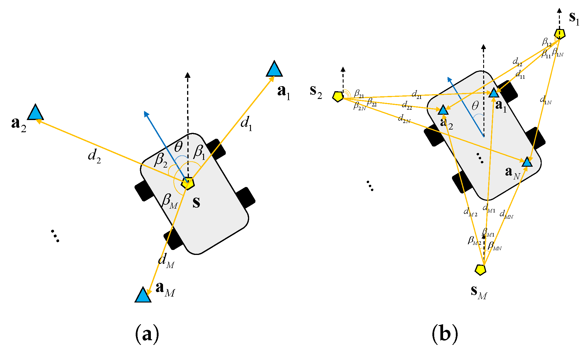
2. Signal Model and Problem Formulation

The main scenarios for two-dimensional (2-D) robot localization are illustrated in Figure 1. In the SL system shown in Figure 1a, there are M tag nodes placed at known positions within the environment, while a single base station is mounted on the robot. In contrast, the traditional RBL system, depicted in Figure 1b, requires N tag nodes on the robot itself and M fixed base stations at known positions [9]. Compared to RBL, the SL approach presented in this paper is simpler and more cost-effective.

The ${\beta }_i$ and $d_i$ are the DS-TWR and measured AOA of the i-th tag, respectively. The coordinates of tags relative to the earth are

$${\mathbf{a}}_i^A={\left[a_{xi}^A,a_{yi}^A\right]}^T,i=1,2,\dots ,M.$$

(1)

The base station is arranged on the robot, whose location $\mathbf{s}={[x,y]}^T$ is unknown, and $\theta$ is the unknown orientation.

To measure the AOAs, the UWB base station communicates with each UWB tag and calculates the phase differences across its antenna elements. The DS-TWR measurements are conducted between the tags and base station in numbered order, respectively. The message-passing and timing measurement model between the base station and tags is illustrated in Figure 2, outlining the process for acquiring both AOA and DS-TWR data.

In the process illustrated in Figure 2, the base station first transmits a beacon frame to initiate communication with the tags. The tags then respond by sending poll frames, allowing the base station to confirm the transmission. Following this, the base station sends a response frame, and the final frames carry the AOA and DS-TWR data for all tags. This process enables precise calculation of the measured distances, denoted as $d_i$ (DS-TWR), between the base station and each tag.

$$d_i={\displaystyle \frac{c}{2}}\left({\displaystyle \frac{R_{is}-D_{si}}{2}}+{\displaystyle \frac{R_{si}-D_{is}}{2}}\right),$$

(2)

where c is the light speed. The measured AOA of i-th tag, ${\beta }_i$, is expressed as follows,

$${\beta }_i={\beta }_i^o+\Delta {\beta }_i,\Delta {\beta }_i\sim \mathcal{N}\left(0,{\sigma }_i^2\right),$$

(3)

where ${\beta }_i^o$ is the true AOA of i-th tag, and $\Delta {\beta }_i$ is the measurement noise, which follows a white Guassian distribution with variance of ${\sigma }_i^2$. The DS-TWR ($d_i$) is assumed to be non-noisy, as the real-life experiments confirm the high accuracy of UWB ranging.

According to Figure 1, the coordinates of tags in the coordinate system of the base station are

$${\mathbf{a}}_i^{Bo}={\left[a_{xi}^{Bo},a_{yi}^{Bo}\right]}^T={\left[d_{i}sin{\beta }_i^o,d_{i}cos{\beta }_i^o\right]}^T,i=1,\dots ,M.$$

(4)

The measurement model for base station with true ${\beta }_i^o$ and $d_i$ is divided into x-axis and y-axis, shown as follows:

$$\begin{array}{cc}\hfill a_{xi}^{Ao}-x& =d_{i}sin\left({\beta }_i^o+\theta \right)\hfill \\ \hfill & =d_{i}sin{\beta }_i^{o}cos\theta +d_{i}cos{\beta }_i^{o}sin\theta \hfill \\ \hfill & =a_{xi}^{Bo}cos\theta +a_{yi}^{Bo}sin\theta ,\hfill \end{array}$$

(5)

$$\begin{array}{cc}\hfill a_{yi}^A-y& =d_{i}cos\left({\beta }_i^o+\theta \right)\hfill \\ \hfill & =d_{i}cos{\beta }_i^{o}cos\theta -d_{i}sin{\beta }_i^{o}sin\theta \hfill \\ \hfill & =-a_{xi}^{Bo}sin\theta +a_{yi}^{Bo}cos\theta .\hfill \end{array}$$

(6)

Stacking the (5) and (6) into the vector ${\mathbf{a}}_i^A$, a simple version of measurement model is

$${\mathbf{a}}_i^A=\mathbf{R}{\mathbf{a}}_i^{Bo}+\mathbf{s},i=1,2,\dots ,M,$$

(7)

where $\mathbf{R}$ is the rotation matrix,

$$\mathbf{R}=\left[\begin{array}{cc}cos\theta & sin\theta \\ -sin\theta & cos\theta \end{array}\right].$$

(8)

To formulate the problem of AOA-TWR-based SL clearly, the measurement model of (7) should be rewritten as

$$\begin{array}{cc}\hfill {\mathbf{a}}_i^A& =\left[\begin{array}{cc}cos\theta & sin\theta \\ -sin\theta & cos\theta \end{array}\right]\left[\begin{array}{c}{a}_{xi}^{Bo}\\ a_{yi}^{Bo}\end{array}\right]+\left[\begin{array}{c}x\\ y\end{array}\right]\hfill \\ \hfill & =\left[\begin{array}{c}{a}_{xi}^{Bo}cos\theta +a_{yi}^{Bo}sin\theta +x\\ -a_{xi}^{Bo}sin\theta +a_{yi}^{Bo}cos\theta +y\end{array}\right]\hfill \\ \hfill & =\left[\begin{array}{cccccc}{a}_{xi}^{Bo}& 0& a_{yi}^{Bo}& 0& 1& 0\\ 0& a_{xi}^{Bo}& 0& a_{yi}^{Bo}& 0& 1\end{array}\right]{\left[\begin{array}{cccccc}cos\theta & -sin\theta & sin\theta & cos\theta & x& y\end{array}\right]}^T\hfill \\ \hfill & ={\mathbf{D}}_i^o\mathbf{f},i=1,2,\dots ,M,\hfill \end{array}$$

(9)

where

$${\mathbf{D}}_i^o=\left[{\mathbf{a}}_i^{BoT}\otimes {\mathbf{I}}_2,{\mathbf{I}}_2\right]\in {\mathbb{R}}^{2\times 6},$$

(10)

is with known variables and

$$\mathbf{f}={\left[\mathrm{vec}{\left(\mathbf{R}\right)}^T,{\mathbf{s}}^T\right]}^T\in {\mathbb{R}}^{6\times 1},$$

(11)

contains all the unknown variables.

By stacking the M tags, the final measurement model of SL based on AOA-TWR is derived for one to solve easily,

$${\mathbf{a}}^A={\mathbf{D}}^o\mathbf{f},$$

(12)

where

$${\mathbf{D}}^o={\left[{\mathbf{D}}_1^{oT},{\mathbf{D}}_2^{oT},\dots ,{\mathbf{D}}_M^{oT}\right]}^T\in {\mathbb{R}}^{2M\times 6},{\mathbf{a}}^A={\left[{\mathbf{a}}_1^{AT},{\mathbf{a}}_2^{AT},\dots ,{\mathbf{a}}_M^{AT}\right]}^T\in {\mathbb{R}}^{2M\times 1}.$$

(13)

With the measurement model in (12), the new problem of AOA-TWR-based SL in this paper is

$$\underset{\mathbf{f}}{min}{∥{\mathbf{a}}^A-{\mathbf{D}}^o\mathbf{f}∥}_2^2.$$

(14)

In the cases without noise, the $\mathbf{f}$ can be obtained easily with a pseudo-linear estimator (PLE):

$$\mathbf{f}={\left({\mathbf{D}}^{oT}{\mathbf{D}}^o\right)}^{-1}{\mathbf{D}}^{oT}{\mathbf{a}}^A.$$

(15)

Unfortunately, the accuracy of (15) is not sufficient, as the measurement noise $\Delta {\beta }_i$ is inevitable in practical cases. In the next section, a robust method is proposed to reduce the impact of noise.

3. SL Algorithm Based on Constrained Weighted Least Squares

In Section 2, the AOA in (15) is considered as a true value. However, in practical cases, the measured AOA is subject to noise, which can significantly affect localization accuracy. This section proposes an enhanced SL algorithm based on CWLS to reduce the impact of measurement noise. First, we analyze the noise model in AOA-TWR-based SL. According to the measured AOAs in (1), the actual ones are

$${\beta }_i^o={\beta }_i-\Delta {\beta }_i,i=1,2,\dots ,M.$$

(16)

Substitute (16) into (4),

$${\mathbf{a}}_i^{Bo}=\left[\begin{array}{c}{d}_{i}sin{\beta }_i^o\\ d_{i}cos{\beta }_i^o\end{array}\right]=\left[\begin{array}{c}{d}_{i}sin\left({\beta }_i-\Delta {\beta }_i\right)\\ d_{i}cos\left({\beta }_i-\Delta {\beta }_i\right)\end{array}\right].$$

(17)

To divide the ${\beta }_i$ and $\Delta {\beta }_i$, we invoke Taylor series expansion and yield

$$\begin{array}{cc}\hfill & sin\left({\beta }_i-\Delta {\beta }_i\right)\approx sin{\beta }_i-\Delta {\beta }_{i}cos{\beta }_i,\hfill \\ \hfill & cos\left({\beta }_i-\Delta {\beta }_i\right)\approx cos{\beta }_i+\Delta {\beta }_{i}sin{\beta }_i.\hfill \end{array}$$

(18)

Thus, (17) becomes

$${\mathbf{a}}_i^{Bo}=\left[\begin{array}{c}{d}_{i}sin{\beta }_i-\Delta {\beta }_i{d}_{i}cos{\beta }_i\\ d_{i}cos{\beta }_i+\Delta {\beta }_i{d}_{i}sin{\beta }_i\end{array}\right]={\mathbf{a}}_i^B-\Delta {\beta }_i{\mathbf{\xi }}_i,$$

(19)

where ${\mathbf{a}}_i^B$ is the coordinate of the i-th tag in the coordinate system of the base station with measured ${\beta }_i$, and ${\mathbf{\xi }}_i={\left[d_{i}cos{\beta }_i,-d_{i}sin{\beta }_i\right]}^T$.

Based on (19), the ${{\mathbf{D}}_i}^0$ in (10) should be expressed with ${\mathbf{D}}_i$ as

$${\mathbf{D}}_i^o={\mathbf{D}}_i-\Delta {\mathbf{D}}_i=\left[{\mathbf{a}}_i^{BT}\otimes {\mathbf{I}}_2,{\mathbf{I}}_2\right]-\left[\Delta {\beta }_i{\mathbf{\xi }}_i^T\otimes {\mathbf{I}}_2,{\mathbf{0}}_{2\times 2}\right].$$

(20)

Then, the ${\mathbf{D}}^0$ in (12) has the form of

$${\mathbf{D}}^o=\mathbf{D}-\Delta \mathbf{D},$$

(21)

where $\mathbf{D}$ has the same form as ${\mathbf{D}}^o$ by substituting ${\beta }_i$ for ${\beta }_i^o$. $\Delta \mathbf{D}$ is the stack of $\Delta {\mathbf{D}}_i,i=1,2,\dots ,M$. For convenience, we express $\Delta \mathbf{D}$ in the manner of matrix multiplication,

$$\Delta \mathbf{D}=\left[\mathbf{\Lambda }\mathbf{B},{\mathbf{0}}_{2M\times 2}\right],$$

(22)

where $\mathbf{\Lambda }=\mathrm{diag}\left(\Delta \mathit{\beta }\right)\otimes {\mathbf{I}}_2\in {\mathbb{R}}^{2M\times 2M}$, $\Delta \mathit{\beta }={\left[\Delta {\beta }_1,\Delta {\beta }_2,\dots \Delta {\beta }_M\right]}^T$ is the vector, and

$$\mathbf{B}={\left[{\mathbf{\xi }}_1^T\otimes {\mathbf{I}}_2;{\mathbf{\xi }}_2^T\otimes {\mathbf{I}}_2;\dots ;{\mathbf{\xi }}_M^T\otimes {\mathbf{I}}_2\right]}^T\in {\mathbb{R}}^{2M\times 4}.$$

(23)

Thus, (12) can be rewritten with (21),

$${\mathbf{a}}^A=\left(\mathbf{D}-\Delta \mathbf{D}\right)\mathbf{f}=\mathbf{Df}-\Delta \mathbf{Df}.$$

(24)

Mathematically, the noisy item can be moved to the right side,

$$\mathbf{Df}-{\mathbf{a}}^A=\Delta \mathbf{Df}.$$

(25)

Finally, the problem model is obtained with a weighted matrix,

$$\underset{\mathbf{f}}{min}g\left(\mathbf{f}\right)={\left(\mathbf{Df}-{\mathbf{a}}^A\right)}^T\mathbf{W}\left(\mathbf{Df}-{\mathbf{a}}^A\right),$$

(26)

where

$$\mathbf{W}={\left(\mathbf{F}\mathbf{\Psi }{\mathbf{F}}^T\right)}^{-1},$$

(27)

and $\mathbf{F}=\mathrm{diag}\left(\mathbf{f}\right)$ is the diagonal matrix of $\mathbf{f}$, $\mathbf{\Psi }=\Delta {\mathbf{D}}^T\Delta \mathbf{D}$. As the $\Delta \mathit{\beta }$ in $\mathbf{\Psi }$ is hard to acquire, we shall rewrite it as

$$\mathbf{\Psi }=\left[\begin{array}{cc}{\mathbf{B}}^T\mathbf{\Xi }\mathbf{B}& \\ & {\mathbf{I}}_2\end{array}\right],$$

(28)

where $\mathbf{\Xi }=\mathbf{Q}\otimes {\mathbf{I}}_2$, and $\mathbf{Q}$ is the covariance matrix of $\Delta \mathit{\beta }$, which is prior knowledge that can be obtained with statistical information.

The $\mathbf{R}$ in $\mathbf{f}$ is the rotation matrix with the characteristics of ${\mathbf{R}}^T\mathbf{R}=\mathbf{I}$ and $det\left(\mathbf{R}\right)=1$ [17]. Thus, the problem of (26) can be formulated as an SL-CWLS model, expressed as follows:

$$\begin{array}{cc}\hfill \underset{\mathbf{f}}{min}& g\left(\mathbf{f}\right)={\left(\mathbf{Df}-{\mathbf{a}}^A\right)}^T\mathbf{W}\left(\mathbf{Df}-{\mathbf{a}}^A\right)\hfill \\ \hfill s.t.& {\mathbf{R}}^T\mathbf{R}=\mathbf{I},\hfill \\ \hfill & det\left(\mathbf{R}\right)=1.\hfill \end{array}$$

(29)

As $\mathbf{R}$ is not suitable for the optimization solver [17], we rewrite the constraints with $\mathbf{f}$. The more solvable SL-CWLS problem is expressed as follows,

$$\begin{array}{cc}\hfill \underset{\mathbf{f}}{min}& g\left(\mathbf{f}\right)={\left(\mathbf{Df}-{\mathbf{a}}^A\right)}^T\mathbf{W}\left(\mathbf{Df}-{\mathbf{a}}^A\right)\hfill \\ \hfill s.t.& {\mathbf{f}}^T{\mathbf{P}}_1\mathbf{f}=1,\hfill \\ \hfill & {\mathbf{f}}^T{\mathbf{P}}_2\mathbf{f}=1,\hfill \\ \hfill & {\mathbf{f}}^T{\mathbf{P}}_3\mathbf{f}=0,\hfill \\ \hfill & {\mathbf{f}}^T{\mathbf{P}}_4\mathbf{f}=1,\hfill \end{array}$$

(30)

where

$$\begin{array}{cc}\hfill & {\mathbf{P}}_1=\mathrm{Diag}\left\{{\mathbf{I}}_{2\times 2},{\mathbf{0}}_{2\times 2},{\mathbf{0}}_{2\times 2}\right\},\hfill \\ \hfill & {\mathbf{P}}_2=\mathrm{Diag}\left\{{\mathbf{0}}_{2\times 2},{\mathbf{I}}_{2\times 2},{\mathbf{0}}_{2\times 2}\right\},\hfill \\ \hfill & {\mathbf{P}}_3=\left[\begin{array}{ccc}0& 1& {\mathbf{0}}_{1\times 4}\\ {\mathbf{0}}_{5\times 1}& {\mathbf{0}}_{5\times 1}& {\mathbf{0}}_{5\times 4}\end{array}\right],\hfill \\ \hfill & {\mathbf{P}}_4=\left[\begin{array}{ccccc}0& 0& 0& 1& {\mathbf{0}}_{1\times 2}\\ 0& 0& -1& 0& {\mathbf{0}}_{1\times 2}\\ {\mathbf{0}}_{4\times 1}& {\mathbf{0}}_{4\times 1}& {\mathbf{0}}_{4\times 1}& {\mathbf{0}}_{4\times 1}& {\mathbf{0}}_{4\times 2}\end{array}\right].\hfill \end{array}$$

(31)

For the moment, we finish the problem formulation of SL-CWLS. Next, (31) is solved with the interior point method, which is summarized in Algorithm 1.

Algorithm 1 SL-CWLS.

Input: Measured AOAs ${\beta }_i,i=1,\dots ,M$, DS-TWRs $d_i,i=1,\dots ,M$, noise variance ${\sigma }^2$. Output: Estimation of $\mathbf{f}$, including location $\mathbf{s}$ and rotation $\mathbf{R}$.      Initialization ${\mathbf{f}}_0$ from (15).      for $t=1:\infty$ do            Construct the Lagrange function of (31)                $\mathcal{L}\left(\mathbf{f},\mathit{\eta }\right)=g\left(\mathbf{f}\right)+{\eta }_1\left({\mathbf{f}}^T{\mathbf{P}}_1\mathbf{f}-1\right)+{\eta }_2\left({\mathbf{f}}^T{\mathbf{P}}_2\mathbf{f}-1\right)+{\eta }_3{\mathbf{f}}^T{\mathbf{P}}_3\mathbf{f}+{\eta }_4\left({\mathbf{f}}^T{\mathbf{P}}_4\mathbf{f}-1\right)$            Construct Karush–Kuhn–Tucker condition.                ${\displaystyle \frac{\partial \mathcal{L}\left(\mathbf{f},\mathit{\eta }\right)}{\partial \mathbf{f}}}=0$,${\mathbf{f}}^T{\mathbf{P}}_1\mathbf{f}=1$,${\mathbf{f}}^T{\mathbf{P}}_2\mathbf{f}=1$,${\mathbf{f}}^T{\mathbf{P}}_3\mathbf{f}=0$,${\mathbf{f}}^T{\mathbf{P}}_4\mathbf{f}=1$.            Newton direction solution with Karush–Kuhn–Tucker condition.                $\left[\Delta {\mathbf{f}}^T,\Delta {\mathit{\eta }}^T\right]=Newton\left({\displaystyle \frac{\partial \mathcal{L}\left(\mathbf{f}\mathit{\eta }\right)}{\partial \mathbf{f}}}\right)$            Update variables.               ${\mathbf{f}}_t={\mathbf{f}}_{t-1}+\vartheta \Delta \mathbf{f}$, ${\mathit{\eta }}_t={\mathit{\eta }}_{t-1}+\vartheta \Delta \mathit{\eta }$            stop condition.                $∥{\displaystyle \frac{\partial \mathcal{L}\left(\mathbf{f},\mathit{\eta }\right)}{\partial \mathbf{f}}}∥\le {\epsilon }_1$ or $∥\Delta \mathbf{f}∥\le {\epsilon }_2$.     end for

4. Constrained Cramér–Rao Lower Bound

In this section, we derive the CCRLB for AOA-TWR-based SL. We first calculate the Cramér–Rao lower bound (CRLB), which provides the theoretical minimum variance achievable for an unbiased parameter estimate. The CRLB is derived for the location $\mathbf{s}$ and rotation $\mathbf{R}$, respectively. In (8), the rotation $\mathbf{R}$ is contained with the trigonometric functions of orientation $\theta$, which can fully represent the $\theta$.

Based on the localization model in (5) and (6), the functions related to the measured angles, ${\beta }_i$s, are given by

$$\begin{array}{cc}\hfill & {\beta }_{xi}^o=arcsin{\displaystyle \frac{\left(a_{xi}^A-x\right)cos\theta -\left(a_{yi}^A-y\right)sin\theta }{d_i}},\hfill \\ \hfill & {\beta }_{yi}^o=arccos{\displaystyle \frac{\left(a_{xi}^A-x\right)sin\theta +\left(a_{yi}^A-y\right)cos\theta }{d_i}}.\hfill \end{array}$$

(32)

Equation (32) is mainly for the estimation of the position vector $\mathbf{s}$, with the DS-TWR measurements $d_i$ to enhance the localization accuracy. For estimating the rotation matrix $\mathbf{R}$, the relationship involving the measured angles, ${\beta }_i$s, are given by

$${\beta }_{\theta i}^o=arctan{\displaystyle \frac{\left(a_{xi}^A-x\right)cos\theta -\left(a_{yi}^A-y\right)sin\theta }{\left(a_{xi}^A-x\right)sin\theta +\left(a_{yi}^A-y\right)cos\theta }}.$$

(33)

For AOA-TWR-based SL, the CRLB can be defined as the inverse of the following Fisher information matrix (FIM),

$$CRLB={\mathcal{F}}^{-1}={\left[\mathbb{E}\left\{{\mathbf{J}}^T{\overline{\mathbf{Q}}}^{-1}\mathbf{J}\right\}\right]}^{-1},$$

(34)

where $\mathbb{E}\left\{·\right\}$ denotes the expectation. The Jacobi matrix is $\mathbf{J}=\left[\begin{array}{cc}{\mathbf{J}}_1& \\ & {\mathbf{J}}_2\end{array}\right]$, where

$${\mathbf{J}}_1=\left[\begin{array}{cccc}{\displaystyle \frac{\partial {\beta }_{\theta 1}^o}{\partial f_1}}& {\displaystyle \frac{\partial {\beta }_{\theta 1}^o}{\partial f_2}}& {\displaystyle \frac{\partial {\beta }_{\theta 1}^o}{\partial f_3}}& {\displaystyle \frac{\partial {\beta }_{\theta 1}^o}{\partial f_4}}\\ ⋮& ⋮& ⋮& ⋮\\ {\displaystyle \frac{\partial {\beta }_{\theta N}^o}{\partial f_1}}& {\displaystyle \frac{\partial {\beta }_{\theta N}^o}{\partial f_2}}& {\displaystyle \frac{\partial {\beta }_{\theta N}^o}{\partial f_3}}& {\displaystyle \frac{\partial {\beta }_{\theta N}^o}{\partial f_4}}\end{array}\right],{\mathbf{J}}_2=\left[\begin{array}{cccc}{\displaystyle \frac{\partial {\beta }_{x1}^o}{\partial f_5}}& {\displaystyle \frac{\partial {\beta }_{x1}^o}{\partial f_6}}& {\displaystyle \frac{\partial {\beta }_{y1}^o}{\partial f_5}}& {\displaystyle \frac{\partial {\beta }_{y1}^o}{\partial f_6}}\\ ⋮& ⋮& ⋮& ⋮\\ {\displaystyle \frac{\partial {\beta }_{xN}^o}{\partial f_5}}& {\displaystyle \frac{\partial {\beta }_{xN}^o}{\partial f_6}}& {\displaystyle \frac{\partial {\beta }_{yN}^o}{\partial f_5}}& {\displaystyle \frac{\partial {\beta }_{yN}^o}{\partial f_6}}\end{array}\right],$$

(35)

and $\overline{\mathbf{Q}}=\left[\begin{array}{cc}\mathbf{Q}& \\ & \mathbf{Q}\end{array}\right]$ is the block diagonal matrix of $\mathbf{Q}$.

According to (32) and (33), the partial differentials are

$$\begin{array}{ccc}\hfill & {\displaystyle \frac{\partial {\beta }_{\theta i}^o}{\partial cos\theta }}={\displaystyle \frac{{\nu }_i\left(a_{xi}^A-x\right)-{\mu }_i\left(a_{yi}^A-y\right)}{{{\mu }_i}^2+{\nu }_i^2}},\hfill & \hfill {\displaystyle \frac{\partial {\beta }_{\theta i}^o}{\partial sin\theta }}={\displaystyle \frac{{\nu }_i\left(a_{yi}^A-y\right)+{\mu }_i\left(a_{xi}^A-x\right)}{{\mu }_i^2+{\nu }_i^2}},\end{array}$$

(36)

$$\begin{array}{ccc}\hfill {\displaystyle \frac{\partial {\beta }_{xi}^o}{\partial x}}& ={\displaystyle \frac{-cos\theta }{\left|{\nu }_i\right|}},{\displaystyle \frac{\partial {\beta }_{xi}^o}{\partial y}}={\displaystyle \frac{sin\theta }{\left|{\nu }_i\right|}},{\displaystyle \frac{\partial {\beta }_{yi}^o}{\partial x}}\hfill & \hfill ={\displaystyle \frac{-sin\theta }{\left|{\mu }_i\right|}},{\displaystyle \frac{\partial {\beta }_{yi}^o}{\partial y}}={\displaystyle \frac{-cos\theta }{\left|{\mu }_i\right|}}.\end{array}$$

(37)

Here, ${\mu }_i=\left(a_{ix}-x\right)cos\theta -\left(a_{iy}-y\right)sin\theta$ and ${\nu }_i=\left(a_{ix}-x\right)sin\theta +\left(a_{iy}-y\right)cos\theta$.

Since in (30), the constraints on $\mathbf{R}$ help promote the performance of CWLS, the CCRLB can be derived based on (34) [23]. Denote $\mathbf{R}=[{\mathbf{r}}_1,{\mathbf{r}}_2]$, and the equality constraints of ${\mathbf{R}}^T\mathbf{R}=\mathbf{I}$ and $det\left(\mathbf{R}\right)=1$ can be re-expressed as the following matrix:

$$\begin{array}{cc}\hfill \mathbf{h}\left(\overline{\mathbf{f}}\right)=& \left[{{\mathbf{r}}_1}^T{\mathbf{r}}_1-1,{{\mathbf{r}}_2}^T{\mathbf{r}}_2-1,{{\mathbf{r}}_1}^T{\mathbf{r}}_2,\mathrm{Det}\left(\mathbf{R}\right)-1\right]\hfill \\ \hfill =& \left[{\overline{\mathbf{f}}}^T{\overline{\mathbf{P}}}_1\overline{\mathbf{f}}-1,{\overline{\mathbf{f}}}^T{\overline{\mathbf{P}}}_2\overline{\mathbf{f}}-1,{\overline{\mathbf{f}}}^T{\overline{\mathbf{P}}}_3\overline{\mathbf{f}},{\overline{\mathbf{f}}}^T{\overline{\mathbf{P}}}_4\overline{\mathbf{f}}-1\right].\hfill \end{array}$$

(38)

Here, $\overline{\mathbf{f}}$ and ${\overline{\mathbf{P}}}_i$ are the expended versions of $\mathbf{f}$ and ${\mathbf{P}}_i$, respectively:

$$\overline{\mathbf{f}}=\left[\mathbf{f};{\mathbf{0}}_{1\times 2}\right],{\overline{\mathbf{P}}}_i=\left[\begin{array}{cc}{\mathbf{P}}_i& \\ & {\mathbf{0}}_{2\times 2}\end{array}\right],i=1,\dots ,4.$$

(39)

The partial differential of (38) is

$$\begin{array}{c}\hfill \mathbf{H}={\displaystyle \frac{\partial \mathbf{h}\left(\overline{\mathbf{f}}\right)}{\partial \overline{\mathbf{f}}}}=\left[2{\overline{\mathbf{P}}}_1\overline{\mathbf{f}},2{\overline{\mathbf{P}}}_2\overline{\mathbf{f}},2{\overline{\mathbf{P}}}_3\overline{\mathbf{f}},2{\overline{\mathbf{P}}}_4\overline{\mathbf{f}}\right].\end{array}$$

(40)

Thus, the CCRLB is

$$CCRLB={\mathcal{F}}^{-1}-{\mathcal{F}}^{-1}\mathbf{H}{\left({\mathbf{H}}^T{\mathcal{F}}^{-1}\mathbf{H}\right)}^{-1}{\mathbf{H}}^T{\mathcal{F}}^{-1}.$$

(41)

The bound on the root mean square error (RMSE) of the rotation matrix $\mathbf{R}$ is

$$\begin{array}{c}\hfill {∥\widehat{\mathbf{R}}-\mathbf{R}∥}_2\ge \sqrt{CCRLB\left(1,1\right)+\dots +CCRLB\left(4,4\right)}.\end{array}$$

(42)

The bound on the RMSE of $\mathbf{s}$ is

$$\begin{array}{cc}\hfill {∥\widehat{\mathbf{s}}-\mathbf{s}∥}_2\ge & {\displaystyle \frac{1}{2}}\left(\sqrt{CCRLB\left(5,5\right)+CCRLB\left(6,6\right)}+\sqrt{CCRLB\left(7,7\right)+CCRLB\left(8,8\right)}\right).\hfill \end{array}$$

(43)

5. Computational Complexity Analysis

In this section, we analyze the computational complexity of the proposed SL-CWLS algorithm.

Table 1. Computational complexities of the considered methods.

Method	Description	Complexity
AVPLE	PLE method in [21] based on AOA	$\mathcal{O}\left(4M\right)$
BCAVPLE-WIV	Two-step method in [21] based on AOA and TWR	$\mathcal{O}\left(M^2+4M\right)$
TELS	Two-step method in [24] based on AOA	$\mathcal{O}\left(M^2+4M\right)$
BC-CWLS	RBL method in [17] based on AOA	$\mathcal{O}\left(T\left({\left(MN\right)}^2+{10}^3\right)\right)$
SL-CWLS	Proposed method based on AOA and TWR	$\mathcal{O}\left(T\left(M^2+5^3\right)\right)$

shows the computation complexities of the methods in this article, and the proposed SL-CWLS, AVPLE, BCAVPLE-WIV [21], TELS [24], and BC-CWLS [17] methods. The PLE requires the computation of $\mathcal{O}\left(M·n^2\right)$, where M is the number of tags and $n=2$ is the problem dimension in this paper. Thus, the AVPLE has the computational complexity of $\mathcal{O}\left(4M\right)$. In the weighted least squares (WLS) step, the complexity of weighted matrix $\mathcal{O}\left(M^2\right)$ is needed with the inversion of the error covariance matrix. Both BCAVPLE-WIV and TELS consist of two steps of PLE and WLS; thus, their complexities are $\mathcal{O}\left(M^2+4M\right)$.

The CWLS method introduces the constraint optimization, which makes its computational complexity higher than WLS. The complexity of CWLS mainly comes from the weighted matrix $\mathcal{O}\left(M^2\right)$ and solving constrained optimization. The $\mathcal{O}\left({ϵ}^3\right)$ is required for the total degree of freedom $ϵ$, which contains the number of problems and constrained conditions. However, the optimization process of CWLS requires several iterations. Assuming the number of iterations is T, the overall complexity of SL-CWLS is $\mathcal{O}\left(T\left(M^2+5^3\right)\right)$. The RBL method of BC-CWLS has M base stations and N tags, as shown in Figure 1b; thus, the complexity with 10 constrains is $\mathcal{O}\left(T\left({\left(MN\right)}^2+{10}^3\right)\right)$. The high complexity of SL-CWLS comes from the iterative solution process of its optimization problem, but at the same time, because of the introduction of constraints, CWLS can provide higher positioning and estimation accuracy, so it is suitable for scenarios with higher precision requirements.

6. Simulation Evaluation

To verify the performances of the proposed SL-CWLS, we carry out the static points and dynamic trajectory simulations, respectively. The proposed SL-CWLS algorithm is compared with AVPLE and BCAVPLE-WIV; TELS is introduced for the AOA-based SL; BC-CWLS is the RBL method which can also provide orientation [17]. The comparisons are conducted with RMSEs of location $\mathbf{s}$ and rotation $\mathbf{R}$ for static points, which agrees with the CCRLB in Section 4. The dynamic trajectories of algorithms are compared with the location $\mathbf{s}$ and orientation $\theta$, which are visible.

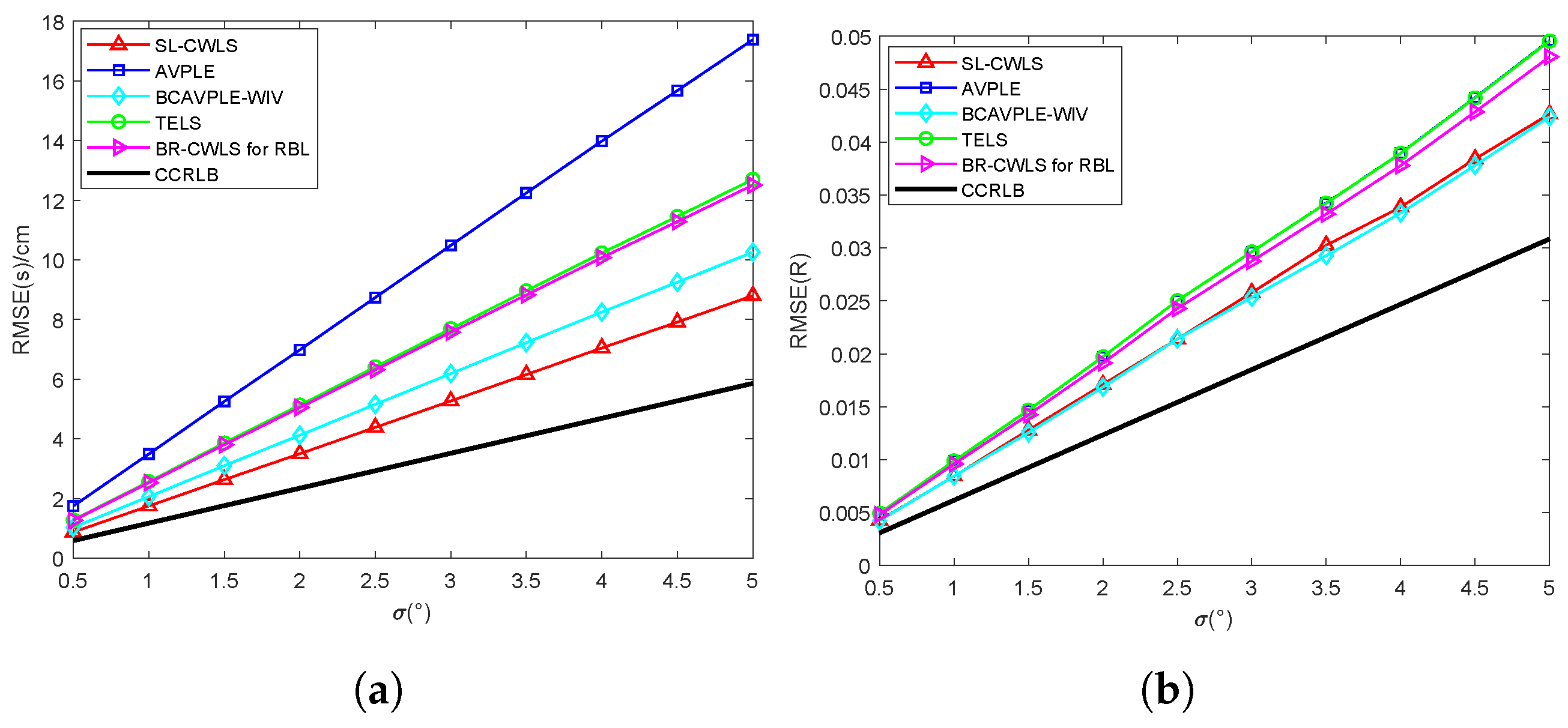
6.1. Static Points Tests

In this subsection, we present simulation results of static points to demonstrate the performance advantages of the proposed SL-CWLS algorithm. The simulations evaluate the accuracies of algorithms under varying AOA noise standard deviations, $\sigma$, and different numbers of tags, M. In the setup, the tags are randomly distributed along the edges of a 320 cm × 320 cm square area, while the base station is fixed at the center with coordinate (160, 160). The results, depicted in Figure 3 and Figure 4, were obtained from 10,000 Monte Carlo trials conducted using MATLAB 2023b. The simulations were performed on a standard PC with an Intel(R) Core(TM) i5-13490 2.5 GHz processor and 32 GB of RAM.

Figure 3 presents the RMSEs of various algorithms with the increasing noise standard deviation $\sigma$ of the AOA. In Figure 3a, the SL-CWLS algorithm achieves the lowest RMSEs for localization, which are the closest to the CCRLB. The BCAVPLE-WIV algorithm shows higher RMSEs compared to SL-CWLS but significantly outperforms both the AVPLE, TELS, and BC-CWLS algorithms. Similarly, in Figure 3b, the RMSE curves of AVPLE and TELS are the highest, while SL-CWLS exhibits RMSEs comparable to those of BCAVPLE-WIV, which are closer to the CCRLB than the AVPLE, TELS, and BC-CWLS. In Table 1, SL-CWLS and BCAVPLE-WIV utilize both the AOA and DS-TWR data for the SL problems, which can significantly improve the accuracy. The AVPLE and TELS estimate the location and rotation with only the AOA; thus, they are inferior to SL-CWLS and BCAVPLE-WIV. These results highlight the effectiveness of the constrained optimization approach employed by SL-CWLS in achieving high localization accuracy. Additionally, the integration of the weighted instrumental variable significantly enhances the performance of BCAVPLE-WIV, representing a notable improvement over the AVPLE [21]. The RBL method BC-CWLS has slightly lower RMSE curves than TELS, as the CWLS can futher reduce the estimation error. It has higher RMSEs than BCAVPLE-WIV and SL-CWLS as the DS-TWRs are not considered.

Figure 4 illustrates the RMSEs of various algorithms with the increasing number of tags, M. In Figure 4a, the RMSEs of all algorithms decrease as M grows, and SL-CWLS achieves the lowest RMSEs. Similarly, Figure 4b shows trends consistent with those in Figure 4a, where the relative performance of the algorithms aligns with the patterns observed in Figure 3b. These results demonstrate that as the number of tags increases, the proposed SL-CWLS algorithm outperforms its counterparts, achieving the most desirable performance.

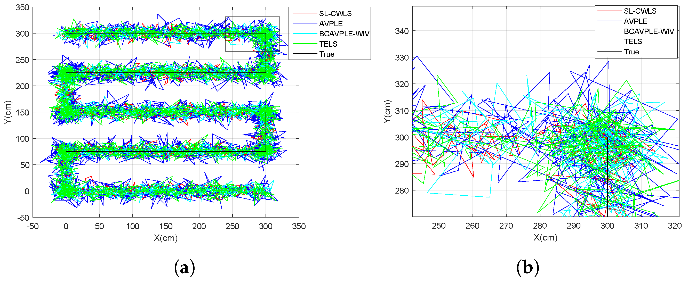
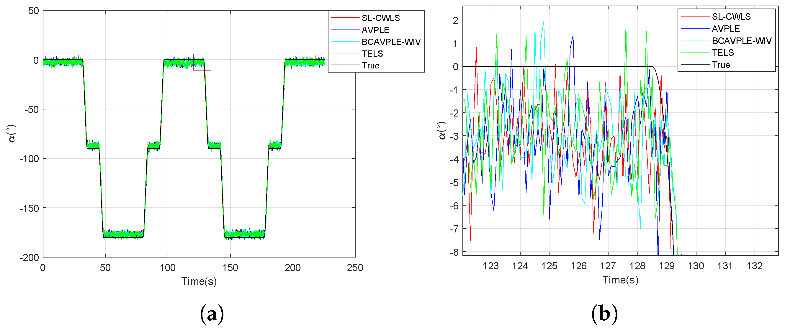
6.2. Dynamic Trajectory Test

In this part, we conduct the dynamic trajectory test for SL-CWLS. We assume that a mobile robot navigates the XoY plane following a zigzag trajectory. The UWB tags are positioned at the four corners of a rectangular court, with coordinates at (−400 cm, 360 cm), (360 cm, 360 cm), (360 cm, −400 cm), and (−400 cm, −400 cm). The robot starts at the position (0 cm, 300 cm) and moves with a max velocity of 10 cm/s. The acceleration is set as 5 cm/s², while the deceleration is 10 cm/s². When the robot turns a corner, its velocity is 0 cm/s, with an angular velocity of 30°/s, an angular acceleration of 30°/s², and an angular deceleration of 30°/s². To simulate the characteristic of UWB, the measurement error of AOA and DS-TWR are set as 5 cm and 5°, respectively. Figure 5a shows the trajectories of algorithms and the true trajectory. The BC-CWLS is not considered as it has relatively high computational complexity, and the performance in Section 6.1 is inferior to SL-CWLS. For careful observation of the details of the trajectories, an enlarged view of the black rectangular box in Figure 5a is depicted in Figure 5b.

From Figure 5a, it can be observed that all trajectories of algorithms are distributed around the true values, with the differences of jump amplitudes. From the enlarged Figure 5b, we can cleary observe that the proposed SL-CWLS has the least jitter amplitudes, and the trajectory of AVPLE has larger amplitudes than other methods. This result is consistent with Figure 3a and Figure 4a.

The joint estimated orientations of corresponding trajectories are depicted in Figure 6a. The rotation comparison in Figure 3b is not visible as the rotation $\mathbf{R}$ is a matrix. Similar to Figure 5b, the enlarged view of the black rectangular box in Figure 6a is depicted in Figure 6b. The orientations of algorithms are all jittered around the true ones, and the AVPLE and TELS seem to have relatively larger jump amplitudes than SL-CWLS and BCAVPLE-WIV.

To clearly demonstrate the dynamic performances of the methods, we analyze the cumulative distribution functions (CDFs), as shown in Figure 7a. It is obvious that SL-CWLS achieves a 90% probability at the RMSE of about 16 cm, which is lower than the 17 cm of BCAVPLE-WIV, 19 cm of TELS, and 27 cm of AVPLE. Similarly, in Figure 7b, SL-CWLS achieves a 90% probability at the lowest orientation RMSE of 5.1°, whereas BCAVPLE-WIV, TELS and AVPLE exhibit RMSEs of 7°, 7.2°, and 7.5°, respectively.

7. Real-World Experiment

In this subsection, we demonstrate the static performance of SL-CWLS in a real-life experiment. First, the experimental UWB equipment is introduced, together with the SL scenario. Then, the results are analyzed for the effectiveness of proposed algorithm.

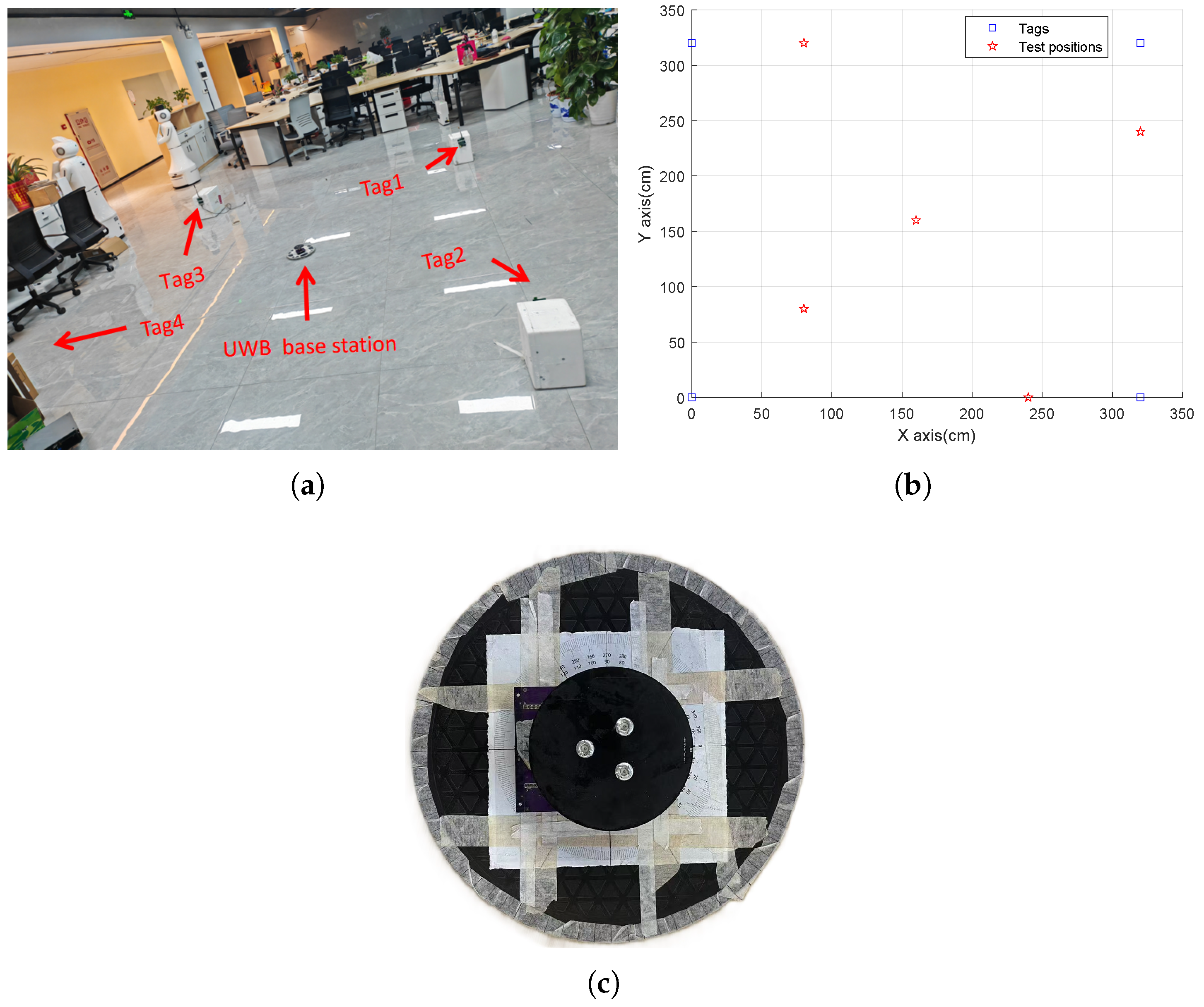
7.1. Experiment Settings

The AOA-TWR-based SL is based on the UWB radar system in Figure 8. Figure 8a shows the self-developed UWB base station with three antennas, which are equipped with DW1000 chips of Decawave company from Ireland. The self-developed tag shown in Figure 8b has one antenna with a DW1000 chip of Decawave. All UWB base stations and tags utilize the IEEE 802.15.4-2011 standard [25]. The system was designed on an STM32 platform, which adopts the STM32F401RCT6 embedded microprocessor, and the 32-bit 256kB microcontroller based on an ARMCortex-M4 core.

Figure 9a depicts the real-world setup for the localization experiment conducted to evaluate the performance of the proposed algorithm. In this experiment, four tags were placed at the corners of a 320 cm × 320 cm square flat surface, while the base station was positioned at the different locations of (80, 320), (160, 160), (80, 80), (240, 0), and (320, 240), as shown in Figure 9b. The real positions were measured with square floor tiles, whose length of sides were measured as 80 cm, within the measurement error of 1 mm. At each position, the orientation angles of the base station were set as 30°, −30°, 60°, and −60° for 1000 trials, respectively. The orientation angles were measured with the dial in Figure 9c, which can guarantee an accuracy of 0.1°.

The AOA measurements of UWB have non-uniform responses for different AOAs. As the base station in Figure 9c is for omnidirectional signals, the performance of the measured AOA of the base station should be analyzed. Figure 10a shows the simulations of RMSEs with AOAs from −180° to 180°, where the SNR = −3 dB, and the result is for 1000 Monte Carlo tests. From the figure, we can find out that the curve has periodic peaks around certain AOAs (60°, 120°, 180°, 0°, −60°, −120°). The three antennas of Figure 9c can obtain three phase differences to calculate the AOA,

$$\begin{array}{c}\hfill {\varphi }_k={\displaystyle \frac{2\pi \varrho cos{\beta }_k}{\lambda }},k=1,2,3,\end{array}$$

(44)

where ${\varphi }_k$ is the k-th phase difference, $\varrho$ denotes the distance between two antennas, and $\lambda$ is the wave length of UWB. The error of AOA measurement is

$$\begin{array}{c}\hfill \left|d{\beta }_k\right|={\displaystyle \frac{\lambda }{2\pi \varrho \left|sin{\beta }_k\right|}}\left|d\varphi \right|,\end{array}$$

(45)

when the incidence AOA ${\beta }_k$ is near 0° and 180° from the line between two antennas, the minimum value of $sin{\beta }_k$ makes the AOA error large. The three lines all have impacts when the AOA is near 0° and 180°, so there are a total of 6 error peaks. Fortunately, when the AOA of one line is near 0° or 180°, the other two lines do not have error peaks. Thus, the accurate AOA measured by the other two lines can be utilized to calculate the AOA. The modified method for measuring the AOA of UWB is to take the mean of the other two AOAs when one of the three measured AOAs is significantly different from the other two. The measured RMSEs for different AOAs of the modified method are depicted in Figure 10b. It can be seen from the figure that the modified method has higher accuracy near the specific angles than what is depicted in Figure 10a.

Table 2. Mean and standard deviation of measured errors of AOAs and DS-TWRs for different orientations.

Positions	Mean of AOA errors (°)				Standard deviation of AOA errors (°)
	30°	−30°	60°	−60°	30°	−30°	60°	−60°
(80,320)	0.0340	0.0480	−0.0463	0.0515	5.0723	5.1210	5.0559	5.0933
(160,160)	0.0453	0.0380	0.0258	−0.0373	5.0935	5.1267	5.0807	5.1010
(80,80)	−0.0418	0.0640	0.0103	0.0473	5.1112	5.0832	5.1210	5.0318
(240,0)	0.0405	0.0175	0.0193	−0.1900	5.0895	5.0687	5.0909	5.0810
(320,240)	0.0475	0.0293	−0.0488	−0.0498	5.1186	5.0357	5.0563	5.0672
	Mean of DS-TWR errors (cm)				Standard deviation of DS-TWR errors (cm)
	30°	−30°	60°	−60°	30°	−30°	60°	−60°
(80,320)	0.4760	−0.4863	0.5005	0.5110	5.0361	5.0628	4.9380	5.0356
(160,160)	−0.5415	0.4058	0.4768	0.4878	4.9482	5.0749	4.9644	5.0428
(80,80)	0.4923	−0.5203	0.5098	−0.5658	5.0476	4.0733	5.0616	5.0496
(240,0)	0.4440	0.4708	−0.5430	0.4785	4.9528	5.0515	5.0426	5.0354
(320,240)	−0.5198	0.5175	−0.5110	0.4883	5.0397	4.9682	5.0569	5.0419

shows the mean and standard deviation of measured errors of AOAs and DS-TWRs for different oritations. From the table, we can find out that the measurement error of the AOA has a nearly zero mean and a 5° standard deviation. This result can indicate the stability of the aforementioned modified method. Moreover, the measurement error of DS-TWR has about a zero mean and a 5 cm standard deviation, which has less impact on estimation than AOAs in practical tests.

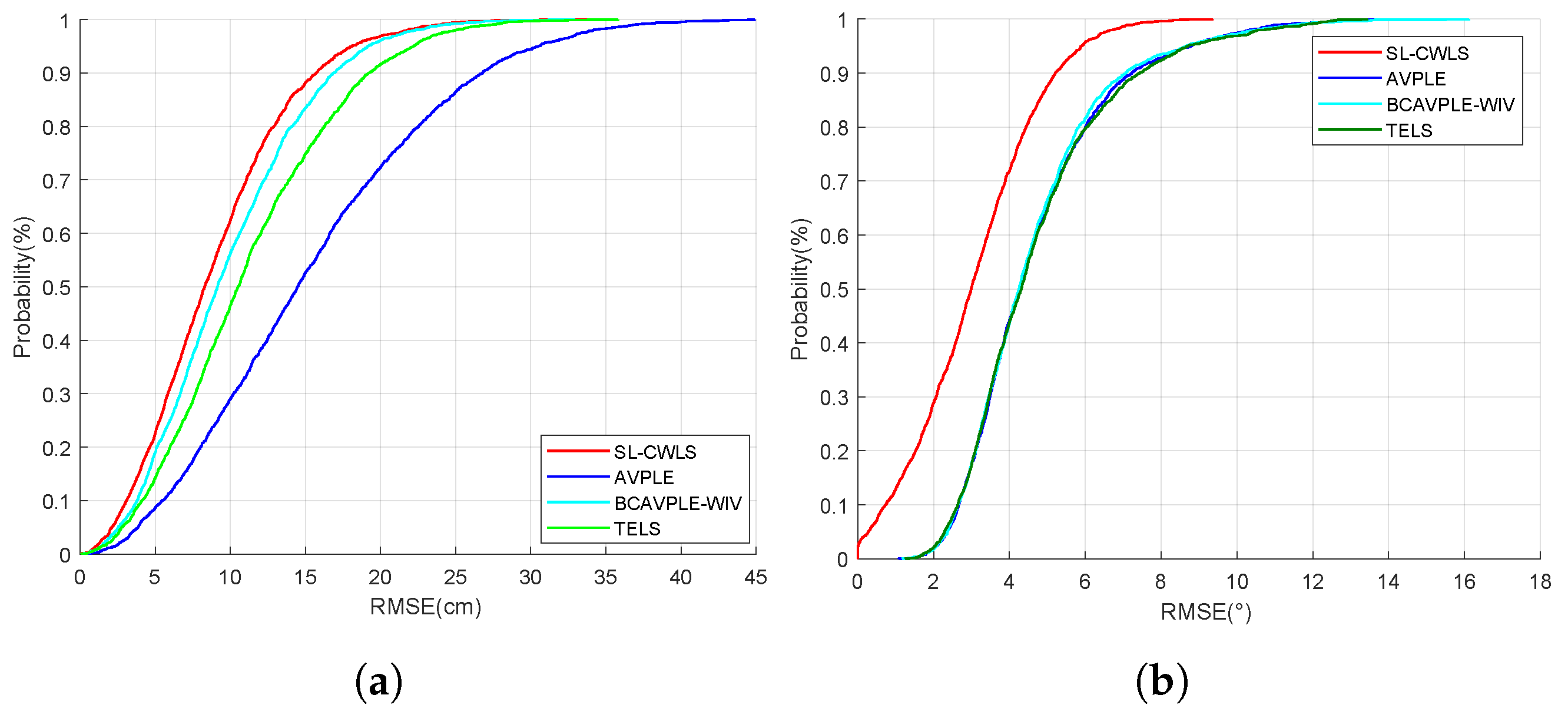
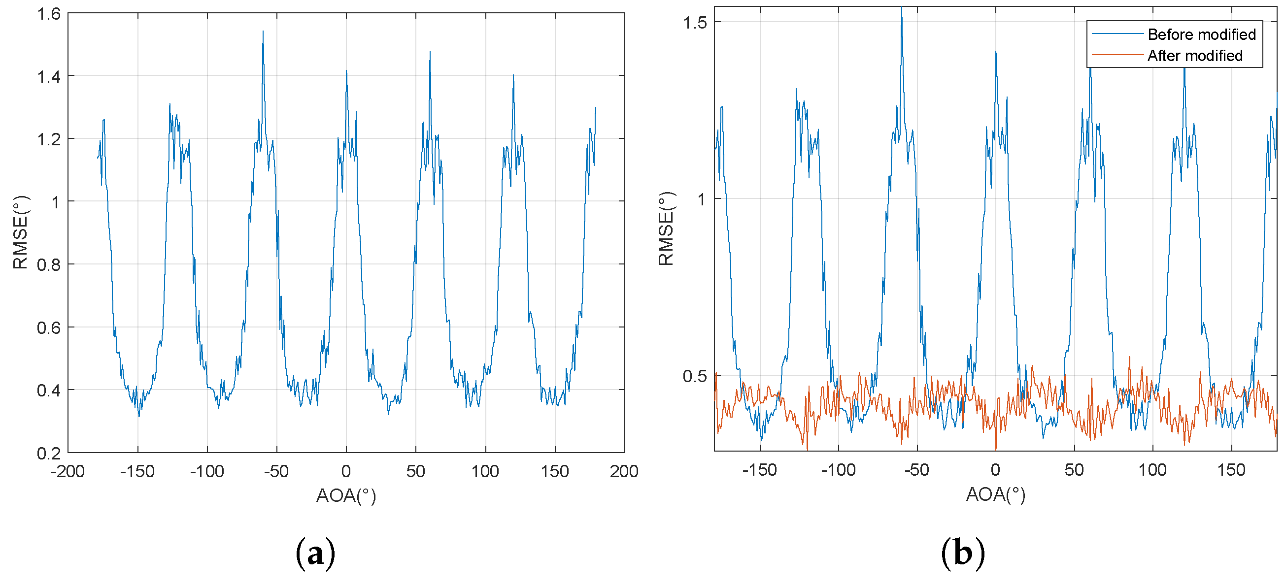
7.2. Analysis of Experimental Results

The RMSEs for $\mathbf{s}$ and $\mathbf{R}$ at each position are summarized in

Table 3. Comparison of RMSEs of location $\mathbf{s}$ for algorithms.

Positions	RMSE (cm)
	AVPLE	BCAVPLE-WIV	TELS	SL-CWLS
(80,320)	27.9279	16.4774	20.2654	13.7289
(160,160)	28.4858	16.8066	20.2518	12.6901
(80,80)	29.2753	17.2724	20.8831	10.5079
(240,0)	31.1556	18.3818	22.4452	8.1818
(320,240)	30.4628	18.0705	22.0644	9.2941

and

Table 4. Comparison of RMSEs of rotation $\mathbf{R}$ for algorithms.

Positions	RMSE
	AVPLE	BCAVPLE-WIV	TELS	SL-CWLS
(80,320)	0.04763	0.04239	0.04760	0.04330
(160,160)	0.04841	0.04309	0.04818	0.04272
(80,80)	0.04887	0.04350	0.04806	0.04443
(240,0)	0.05410	0.04815	0.05104	0.04806
(320,240)	0.05254	0.04346	0.04964	0.04335

, which are the mean results of all orientation angles. The noise standard deviation for the measured angles ${\beta }_i$s, is set to $\sigma$ = 5° for all tests. Note that the bold numbers of RMSE are the least in one position. Table 3 and Table 4 highlight that the proposed SL-CWLS algorithm achieves the most accurate localization RMSEs among all tested algorithms across all base station positions, reaching centimeter-level accuracy at positions (240, 0) and (320, 240). The rotation RMSEs at positions (80, 320) and (80, 80) are slightly higher than those of BCAVPLE-WIV. These findings demonstrate the effectiveness of the constrained optimization of SL-CWLS, as detailed in Section 6.1. In contrast, the AVPLE has less stable performance, with the highest RMSEs for both position and rotation. These trends align with the results shown in Figure 3 and Figure 4.

8. Conclusions

This paper addresses a novel problem in AOA-TWR-based localization and orientation estimation for UWB systems in robotic applications. To tackle this problem, we propose a new algorithm termed SL-CWLS, which employs a weighted matrix and constrained convex optimization to achieve high accuracy. Moreover, a CCRLB is derived as a benchmark for the performance of SL-CWLS. Simulation results demonstrate that SL-CWLS achieves the lowest RMSEs for localization and exhibits robust performance in rotation estimation, both in static and dynamic scenarios. In real-world experiments, the SL-CWLS outperforms counterparts, achieving centimeter-level localization accuracy and delivering reliable rotation estimation. Future research will focus on developing advanced methods for localization and orientation estimation, particularly for 3D scenario and non-line-of-sight (NLOS) problems, and based on machine learning techniques.

References

1. Liu, A.; Wang, J.; Lin, S.; Kong, X. A dynamic UKF-based UWB/wheel odometry tightly coupled approach for indoor positioning. Electronics 2024, 13, 1518. [Google Scholar] [CrossRef]
2. Win, M.Z.; Scholtz, R.A. Ultra-wide bandwidth time-hopping spread-spectrum impulse radio for wireless multiple-access communications. IEEE Trans. Wireless Commun. 2000, 48, 679–689. [Google Scholar] [CrossRef]
3. Zafari, F.; Gkelias, A.; Leung, K.K. A Survey of Indoor Localization Systems and Technologies. IEEE Commun. Surveys Tutorials 2019, 21, 2568–2599. [Google Scholar] [CrossRef]
4. Davide, S.; Stefano, M.; Vineeth, T.; Upadhyay, P.K.; Magarini, M. Experimental comparison of UAV-Based RSSI and AOA localization. IEEE Sens. Lett. 2024, 8, 1–4. [Google Scholar]
5. Chehri, A.; Fortier, P.; Tardif, P.M. On the TOA estimation for UWB ranging in complex confined area. In Proceedings of the 2007 International Symposium on Signals, Systems and Electronics, Montreal, QC, Canada, 30 July–2 August 2007; pp. 533–536. [Google Scholar]
6. Ma, T.; Zhang, D.; Zhuang, J.; You, C.; Yin, G.; Tang, S. TDOA-based UWB indoor 1D localization via weighted sliding window filtering. Digital Signal Process. 2024, 151, 104544. [Google Scholar] [CrossRef]
7. Smaoui, N.; Heydariaan, M.; Gnawail, O. Single-antenna AOA estimation with UWB radios. In Proceedings of the 2021 IEEE Wireless Communications and Networking Conference (WCNC), Nanjing, China, 29 March 2021–1 April 2021; pp. 1–7. [Google Scholar]
8. Igor, D.; Andrew, C.; Ma, H.; Jeff, C.; Michael, M. Angle of arrival estimation using decawave DW1000 integrated circuits. In Proceedings of the 2017 14th Workshop on Positioning, Navigation and Communications (WPNC), Bremen, Germany, 26 October 2017; pp. 1–6. [Google Scholar]
9. Wang, T.; Zhao, H.; Shen, Y. An efficient single-anchor localization method using ultra-wide bandwidth systems. Appl. Sci. 2020, 10, 57. [Google Scholar] [CrossRef]
10. Sun, Y.; Ho, K.C.; Wan, Q. Eigenspace solution for AOA localization in modified polar representation. IEEE Trans. Signal Process. 2020, 68, 2256–2271. [Google Scholar] [CrossRef]
11. Zheng, Y.; Sheng, M.; Liu, J.; Li, J. Exploiting AOA Estimation Accuracy for Indoor Localization: A Weighted AOA-Based Approach. IEEE Wireless Commun. Lett. 2019, 8, 65–68. [Google Scholar] [CrossRef]
12. Zou, Y.; Wu, W.; Zhang, Z. Source Localization Based on Hybrid AOA, TDOA, and RSS Measurements. IEEE Sens. J. 2023, 23, 16293–16302. [Google Scholar] [CrossRef]
13. Zou, Y.; Wu, W.; Fan, J.; Liu, H. Constrained Weighted Least-Squares Algorithms for 3-D AOA-Based Hybrid Localization. IEEE Open J. Signal Process. 2024, 5, 436–448. [Google Scholar] [CrossRef]
14. Alonge, F.; D’Ippolito, F.; Garraffa, G.; Sferlazza, A. Hybrid Observer for Indoor Localization with Random Time-of-Arrival Measurments. In Proceedings of the 2018 IEEE 4th International Forum on Research and Technology for Society and Industry (RTSI), Palermo, Italy, 10–13 September 2018; pp. 1–6. [Google Scholar]
15. Zhou, B.; Fang, H.; Xu, J. UWB-IMU-Odometer Fusion Localization Scheme: Observability Analysis and Experiments. IEEE Sens. J. 2023, 23, 2550–2564. [Google Scholar] [CrossRef]
16. Zhou, B.; Ai, L.; Dong, X.; Yang, L. DoA-based rigid body localization adopting single base station. IEEE Commun. Lett. 2019, 23, 494–497. [Google Scholar] [CrossRef]
17. Wang, G.; Ho, K.C.; Chen, X. Bias reduced semidefinite relaxation method for 3-D rigid body localization using AOA. IEEE Trans. Signal Process. 2021, 69, 3415–3430. [Google Scholar] [CrossRef]
18. Chepuri, S.P.; Leus, G.; van der Veen, A.-J. Rigid Body Localization Using Sensor Networks. IEEE Trans. Signal Process. 2014, 62, 4911–4924. [Google Scholar] [CrossRef]
19. Jiang, H.; Wang, W.; Shen, Y.; Li, X.; Ren, X.; Mu, B. Efficient Planar Pose Estimation via UWB Measurements. In Proceedings of the 2023 IEEE International Conference on Robotics and Automation (ICRA), London, UK, 29 May–2 June 2023; pp. 1954–1960. [Google Scholar]
20. Abouzar, P.; Michelson, D.G.; Hamdi, M. RSSI-Based Distributed SL for Wireless Sensor Networks Used in Precision Agriculture. IEEE Trans. Wireless Commun. 2016, 15, 6638–6650. [Google Scholar] [CrossRef]
21. Shao, H.; Zhang, X.; Wang, Z. Efficient closed-form algorithms for AOA based SL of sensor nodes using auxiliary variables. IEEE Trans. Signal Process. 2014, 62, 2580–2594. [Google Scholar] [CrossRef]
22. Taponecco, L.; D’Amico, A.A.; Mengali, U. Joint TOA and AOA Estimation for UWB Localization Applications. IEEE Trans. Wireless Commun. 2011, 10, 2207–2217. [Google Scholar] [CrossRef]
23. Wang, G.; Ho, K.C. Accurate semidefinite relaxation method for rigid body localization using AOA. In Proceedings of the 2020 IEEE International Conference on Acoustics, Speech and Signal Processing (ICASSP), Barcelona, Spain, 4–8 May 2020; pp. 4955–4959. [Google Scholar]
24. Watanabe, F. Wireless Sensor Network Localization Using AoA Measurements With Two-Step Error Variance-Weighted Least Squares. IEEE Access 2021, 9, 10820–10828. [Google Scholar] [CrossRef]
25. IEEE Std 802.15.4-2011 (Revision of IEEE Std 802.15.4-2006); IEEE Standard for Local and metropolitan area networks–Part 15.4: Low-Rate Wireless Personal Area Networks (LR-WPANs). IEEE: New York, NY, USA, 2011; pp. 1–314.
Figure 1. Main scenarios of robot localization. (a) SL. (b) RBL.
Electronics 14 00429 g001
Figure 2. Message-passing and timing measurement of UWB for AOA-TWR localization model.
Electronics 14 00429 g002
Figure 3. RMSE v.s. noise standard deviation  σ  for algorithms. (a) Location  s . (b) Rotation  R .
Electronics 14 00429 g003
Figure 4. RMSE v.s. number of tags, M, for algorithms. (a) Location  s . (b) Rotation  R .
Electronics 14 00429 g004
Figure 5. Dynamic trajectories of algorithms. (a) Trajectories. (b) Enlarged view of (a).
Electronics 14 00429 g005
Figure 6. Dynamic orientations of algorithms. (a) Orientations. (b) Enlarged view of (a).
Electronics 14 00429 g006
Figure 7. CDFs of algorithms. (a) Trajectories. (b) Orientations.
Electronics 14 00429 g007
Figure 8. UWB devices for AOA-TWR-based SL. (a) Three-antenna UWB base station, (b) UWB label.
Electronics 14 00429 g008
Figure 9. AOA-TWR-based SL scenario based on UWB. (a) Real scenario, (b) Test positions of base station. (c) Measurement dial for orientation angles of base station in (a).
Electronics 14 00429 g009
Figure 10. RMSEs for different AOAs in simulation for Figure 9c. (a) Trajectories. (b) Orientations.
Electronics 14 00429 g010