Article

A CNN-GRU Model-Based Trajectory Error Predicting and Compensating for a 6-DOF Parallel Robot

1
Tianjin Research Institute for Water Transport Engineering, M.O.T., Tianjin 300456, China
2
Institute of Mechanics and Acoustic Metrology, National Institute of Metrology, Beijing 100029, China
3
Guizhou Institute of Metrology, Guiyang 550003, China
*
Author to whom correspondence should be addressed.
Electronics 2025, 14(23), 4752; https://doi.org/10.3390/electronics14234752
Submission received: 6 October 2025 / Revised: 25 November 2025 / Accepted: 28 November 2025 / Published: 3 December 2025

Abstract

The six-degree-of-freedom parallel robots is crucial for intelligent manufacturing, motion simulation, aerospace and other fields. Their trajectory performance level directly affects the reliable application of high-precision operation scenarios. However, dynamic trajectory errors under motion conditions remain a challenge. To address this, to improve the motion trajectory accuracy of parallel robots, a CNN-GRU model-based trajectory error prediction and compensation method is proposed. The novelty of this method lies in the hybrid deep learning architecture that combines CNN for spatial feature extraction and GRU for temporal dependency modeling. This method accurately predicts the trajectory error of parallel robots by constructing a deep learning model that integrates CNN and GRU, and compensates for the amplitude and bias of the trajectory error at the control command end, thereby improving the trajectory accuracy of parallel robots. The simulation and the 6-UPS parallel robot experiment verified the effectiveness of the proposed trajectory error prediction and compensation method. Key findings showed that the accuracy of the sinusoidal trajectory and circular trajectory of the parallel robot after error compensation was improved by about 90%.

1. Introduction

Parallel robots are renowned for their high stiffness, high payload-to-weight ratio, and superior dynamic performance, affording them significant advantages in the high-quality manufacturing of large, complex aerospace components. They are widely employed in applications such as motion simulation [1], high-precision assembly [2,3,4], and aviation testing [5]. However, during actual production and manufacturing processes, these robots inevitably suffer from errors induced by sources such as manufacturing and link deviations. These errors directly impact the performance of application systems reliant on the motion trajectory of parallel robots, potentially leading to significant and difficult-to-quantify losses. Consequently, high-precision error compensation for parallel robots is of paramount importance for applications including high-accuracy machining, inertial navigation test systems, and precision positioning.
Error compensation for parallel robots is generally categorized into online and offline methods [6,7]. Online compensation typically employs additional measurement devices to monitor the robot’s absolute position for trajectory error correction [8,9,10]. This approach heavily depends on the accuracy of external measurement equipment, limiting its applicability in complex industrial environments. Furthermore, as the control signal is calculated based on the error measured in the preceding time step, the corrective action invariably lags behind the error occurrence; that is, compensation is applied after the control operation. In contrast, offline compensation preemptively addresses potential errors to enhance robot performance. It predicts pose errors and implements corrections in advance, thereby applying corrective actions before errors manifest. Offline pre-compensation methods are generally subdivided into model-based and model-free approaches, with the latter further encompassing techniques such as curve fitting, neural networks, and spatial interpolation [11].
Model-based error parameter identification methods primarily involve four steps: error modeling, pose measurement, parameter identification, and parameter compensation. For instance, Qiang H et al. [12] developed a dimensionless error model for the Stewart platform based on the differential closed-loop vector equation, and identified the error parameters using the least squares method for compensation. He et al. [13] investigated a kinematics calibration method based on the finite instantaneous screw, constructing an error model through the error mapping of serial chains. They categorized redundant errors into intra- and inter-chain errors, defined a minimum identification model, and achieved error transfer compensation. Fu et al. [14] developed a pose measurement method for a 6-DOF parallel robot using binocular vision, accurately measuring the moving platform’s pose. They established a dimensionless error model based on the robot’s structural characteristics to improve the accuracy of geometric parameter error identification. However, as error models do not encompass all error sources and measurement equipment itself introduces inevitable inaccuracies, uncertainty in error parameter identification is increased. Moreover, these parameter identification methods inevitably overlook error sources such as elastic deformations and clearances in the transmission system, resulting in limited improvements in pose accuracy.
Model-free error compensation methods, conversely, circumvent the need to consider specific error sources by utilizing data-driven models for robot error prediction. Alici et al. [15] proposed representing end-effector positioning errors using Fourier and ordinary polynomials, estimating pose errors at arbitrary points within the workspace based on curve fitting results. Hu et al. [16] investigated a positioning error compensation method for industrial robots using a genetic algorithm-particle swarm optimization-deep neural network (GA-PSO-DNN). By analyzing the influence of target pose on error via Latin hypercube sampling, they reduced the pose positioning error by 77.57%. Dolinsky et al. [17] studied a genetic algorithm-based error compensation method, establishing a mapping between end-effector pose error and individual joint errors, and compensated for the robot’s pose error accordingly. Zhou et al. [18] avoided constructing complex error compensation models by integrating spatial interpolation with similarity-based interpolation weights. Li et al. [19] developed a neural network-based robot error compensation method, utilizing predicted errors to compensate for target points within the workspace. Yu [20] constructed a hybrid network model comprising artificial neural networks and radial basis function networks to predict static pose errors caused by non-geometric parameters. Zhu et al. [21,22] proposed a pose error prediction and compensation method for parallel robots based on deep learning, using a neural network to predict static pose errors and enhancing static pose accuracy through pre-compensation. However, these methods primarily focus on predicting and compensating for static pose errors, with limited investigation into trajectory error prediction and compensation under dynamic conditions.
To enhance the motion trajectory performance of parallel robots, this study proposes a trajectory error prediction and compensation method based on a CNN-GRU (Convolutional Neural Network and Gated Recurrent Unit) model. Firstly, a trajectory error prediction model integrating CNN and GRU is constructed. This model combines the spatial feature extraction capability of convolutional neural networks with the temporal dynamic capture ability of gated recurrent units to accurately predict trajectory errors. Whereafter, a trajectory error dataset for the robot is built, comprising desired trajectories and the corresponding measured actual trajectory errors, which are then used to train the model. Finally, a method involving direct modification of the commanded trajectory input to the controller is adopted to achieve dual compensation for both the magnitude and bias of the parallel robot’s trajectory error, thereby enhancing its trajectory accuracy.

2. Proposed Methodology

2.1. 6-UPS Parallel Robot and Its Kinematic Model

2.1.1. 6-UPS Parallel Robot

Six-degree-of-freedom (6-DOF) parallel robots play an indispensable role in practical industrial applications [23] and are commonly referred to as Stewart platforms. Figure 1 illustrates the architecture of a 6-UPS parallel robot, which consists of a movable platform, a fixed base, spherical joints, Universal joints, electric cylinders, and servo motors. The movable platform is connected to the fixed base by six independently driven limbs, each capable of linear extension and retraction. By precisely controlling the length of these six limbs, the movable platform can achieve translational motion along the x-, y-, and z-axes, as well as rotational motion about these three axes, enabling comprehensive 6-DOF pose adjustment. The pose of the movable platform is denoted by Q (x, y, z, α, β, γ), where x, y, and z represent its positional coordinates, while α, β, and γ represent the rotation angles about the x-, y-, and z-axes, respectively. The orientation of the parallel robot is described using Euler angles.

2.1.2. Kinematic Analysis of the 6-UPS Parallel Robot

The kinematics of parallel robots is divided into forward and inverse kinematics. The former determines the pose of the movable platform from the lengths of the six driving limbs, while the latter computes the required limb lengths from a given platform pose. For a six-degree-of-freedom parallel robot, the inverse kinematics admits a closed-form analytical solution, whereas the forward kinematics lacks an exact analytical solution and must be solved using numerical methods.
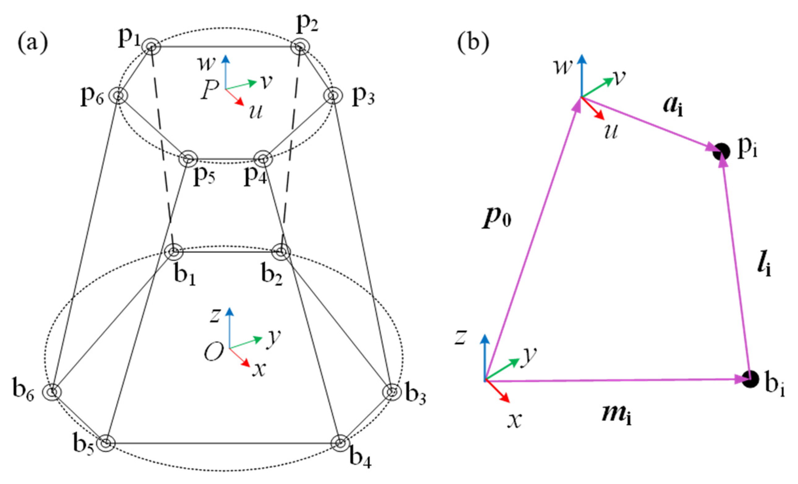
To derive the inverse kinematics of the parallel robot, its mechanism is simplified as shown in Figure 2a, where ai (i = 1, 2, …, 6) denotes the center of the spherical joint, and bi represents the center of the Universal joint. To formulate the kinematic equations, coordinate systems P-uvw and O-xyz are established at the center of the movable platform and the fixed base, respectively. The vector loop of a limb is illustrated in Figure 2b: the vector from origin O to bi is denoted as mi, the vector from O to P is denoted as p0, and the vector from pi to bi is denoted as li. The vector loop equation for a limb of the parallel robot is expressed as follows:
l i = p 0 + Ra i m i         i = 1 ,   2 , 6
  • ai is the position vector of the spherical joint center expressed in the movable platform coordinate system P-uvw.
  • R is the rotation matrix of the movable platform coordinate system P-uvw with respect to the fixed-base coordinate system O-xyz. The homogeneous transformation matrix T which combines both rotation and translation, and can be expressed as:
T = R p 0 0 1 = c γ c β c γ s β s α s γ c α c γ s β c α + s γ s α x s γ c β s γ s β s α + c γ c α s γ s β c α c γ s α y s β c β s α c β c α z 0 0 0 1
where p0 = [x,y,z]T is the position vector of the movable platform origin expressed in the base coordinate system, R is the rotation matrix defined above, s and c denote the sin and cos functions, respectively, and the angles α, β, γ ∈ [0, π].
For a prescribed pose Q (x, y, z, α, β, γ), the actuator length is given by:
l i = p 0 + Ra i   m i
For any prescribed set of six actuator lengths ln (1, 2, …, 6), the forward kinematic model of the parallel robot is formulated as:
f ( x , y , z , α , β , γ )   =   p 0 + R a i   m i l n = 0
Equation (4) thereby enables the transformation of the forward kinematics problem into a minimization problem, which is subsequently solved using numerical methods to determine the actuator lengths. For the specific computational procedure of the parallel robot’s forward kinematics solution, Fu et al. [24] have provided a detailed elaboration.

2.2. CNN-GRU Model-Based Trajectory Error Prediction

2.2.1. Convolutional Neural Network (CNN)

The CNN possess a hierarchical feature learning capability, and its core architecture is composed of convolutional layers, pooling layers, activation function modules, and fully connected layers, enabling the automatic extraction of multi-faceted and deep-level features from raw data [25].
Convolutional Layer: this is the most critical component, performing convolution operations to capture spatial features from adjacent points in the input vector. It operates by applying multiple learnable convolutional kernels that locally perceive the input data. The mechanism of weight sharing within these kernels effectively reduces the number of model parameters. The operation computed the dot product between the input data and the kernel weight matrix, expressed as:
x i t = σ ( j = 1 n w i j t x j t 1 + b i t )
  • x i t denotes the i-th output in the t-th layer.
  • x j t 1 denotes the j-th output in the (t-1)-th layer.
  • w ij t represents the weight matrix of the convolutional kernel.
  • b i t represents the bias of the convolutional kernel.
  • ∗ denotes the dot product operation.
  • σ represents the activation function.

2.2.2. Gated Recurrent Unit (GRU)

The Gated Recurrent Unit (GRU) offers distinct advantages in processing sequential data and capturing temporal dependencies. As a variant of the Long Short-Term Memory (LSTM) network, it effectively addresses the common challenges in standard Recurrent Neural Networks (RNNs), namely the vanishing/exploding gradient problem and the difficulty in modeling long-range dependencies. Furthermore, GRU employs a streamlined gating mechanism and recurrent unit design that optimizes the network architecture, enhances the transferability of RNN models, and provides a more compact and computationally efficient framework compared to LSTM. This design enables GRU to balance applicability with training efficiency while effectively mitigating overfitting tendencies [26]. The core operations of the GRU are formulated as follows:
z k = S i g ( W z ·   [ c k 1 ,   x k ] )
c ˜ k = tanh ( W ·   [ r k c k 1 ,   x k ] )
r k = S i g ( W r ·   [ c k 1 ,   x k ] )
c k = ( 1 z k ) c k 1 + z k c ˜ k
  • Sig denotes the Sigmoid activation function.
  • ck represents the memory state.
  • zk and rk are the update gate and reset gate, respectively.
  • Wr, Wz, and W denote the weight matrices.
  • xk is the input to the neuron at step k.
  • tanh is the hyperbolic tangent activation function.
  • yk is the output of the neuron.
  • c k denotes the memory gate.
  • signifies the element-wise multiplication operation.

2.2.3. CNN-GRU Model

Figure 3 illustrates the fundamental architecture of the CNN-GRU model, which is primarily constructed by integrating a CNN layer, a GRU layer, and fully connected layers. The CNN layer projects the one-dimensional pose data into a high-dimensional feature space. Leveraging its local receptive fields, it effectively extracts the spatial coupling characteristics among pose parameters. This feature extraction process considers not only variations in individual parameters but also captures interrelationships among multiple parameters, thereby providing rich informational features for subsequent error prediction. While GRU networks exhibit strong capabilities in processing sequential data, practical trajectory error measurements inevitably introduce device measurement noise, which can compromise the prediction accuracy of a standalone GRU model. Consequently, the integration of CNN with GRU effectively mitigates interference from measurement noise, enabling reliable prediction of the parallel robot’s trajectory error.

3. Simulation Validation

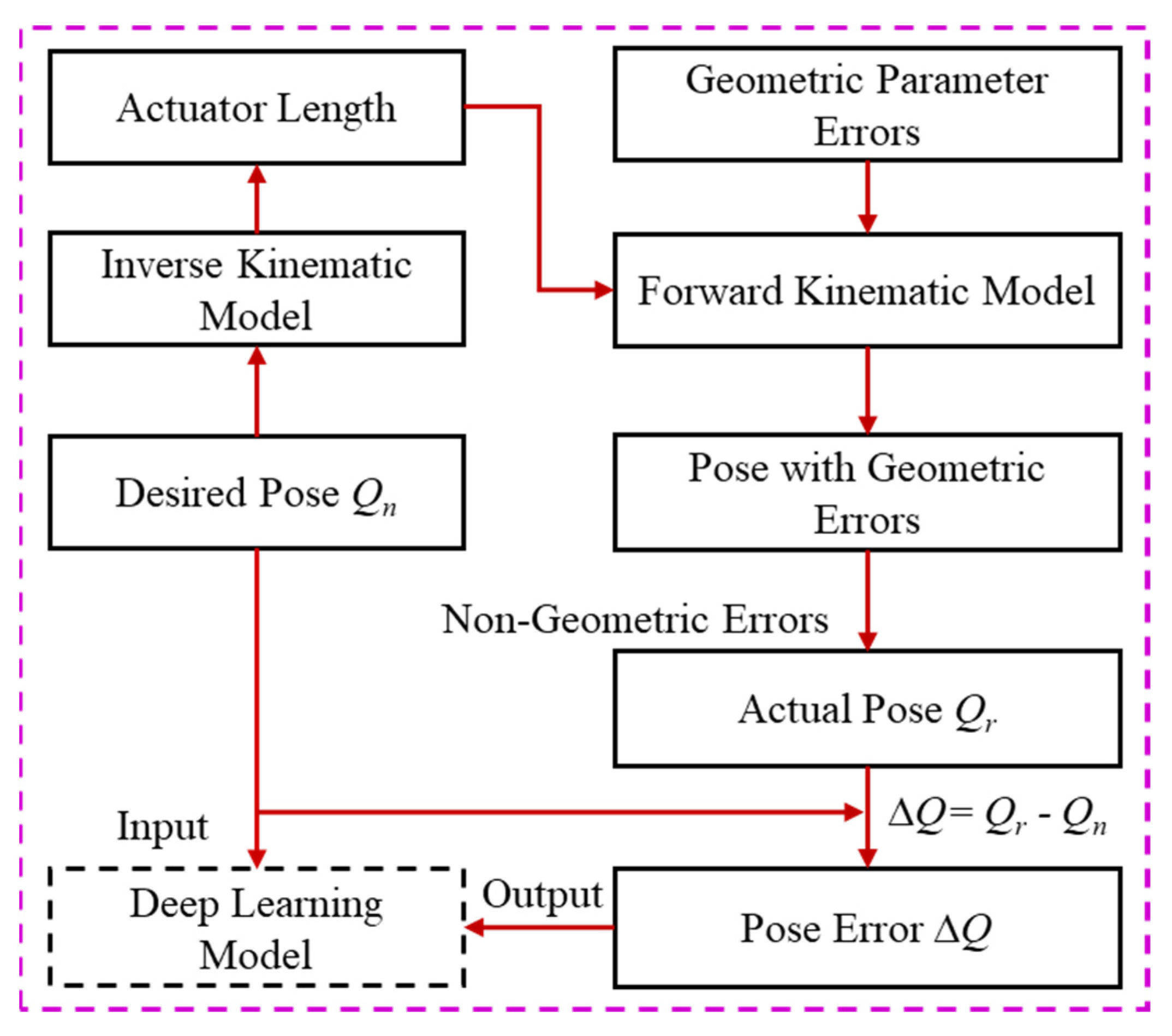
Figure 4 illustrates the process of simulation data generation and model training. By incorporating simulated geometric parameter errors into the nominal forward kinematic model, this process effectively simulates the impact of geometric errors on the platform pose.
The geometric parameter errors of the 6-UPS parallel robot include the position errors of the upper and lower spherical joints, denoted as Δaix, Δaiy, Δaiz, Δbix, Δbiy, Δbiz and the actuator length error Δli. Each kinematic chain comprises seven error parameters, resulting in a total of 42 geometric error parameters. The geometric parameter errors utilized in the forward kinematic model are listed in Table 1. The simulation procedure is conducted as follows: Firstly, the desired trajectory is discretized into a sequence of desired poses Qn, and the corresponding actuator lengths are computed via inverse kinematics. Subsequently, the pose error is calculated by generating simulated poses using the forward kinematic model incorporating the geometric errors. Simulated non-geometric errors, ranging from −0.04 to 0.04 mm, are then added to these poses to reflect dynamic variations. Finally, a dataset composed of the desired poses and their corresponding pose errors is constructed to train the CNN-GRU model. The hyperparameters for the model are detailed in Table 2. Based on the model configuration provided in Table 2, single-sample inference on a modern GPU requires only about 1–2 ms, indicating that the model is capable of real-time trajectory error prediction and compensation.
The convolutional kernel sizes are uniformly set to 3 × 1, with the number of kernels configured as 6 and 3, respectively. The GRU layer consists of 6 fundamental GRU. The model is trained with a batch size of 32. The Adam optimizer is employed for parameter optimization during training, with key parameters including the initial learning rate, decay rate, and decay steps. When the number of training epochs reaches the specified decay steps, the learning rate is automatically adjusted by multiplying the current learning rate by the decay rate to generate a new learning rate. This scheduling strategy ensures training stability and promotes effective convergence. The network is trained using the Mean Absolute Error (MAE) loss function, which provides robust gradient behavior and improves prediction stability for trajectory error estimation.
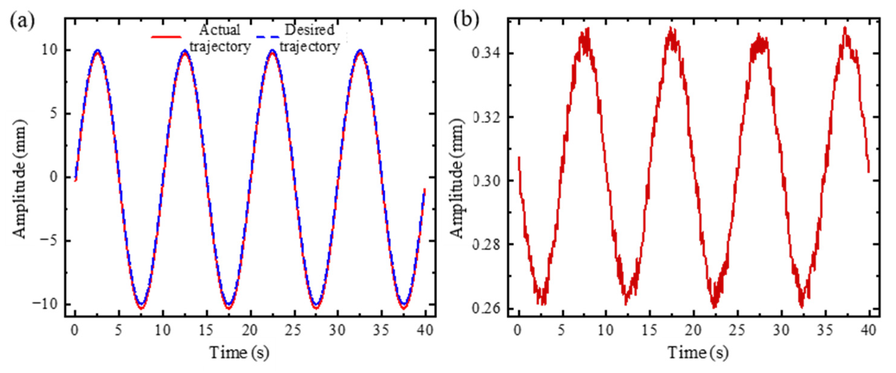
Figure 5 displayed the actual trajectory and trajectory error of the parallel robot under sinusoidal motion with a 10 mm amplitude. The sinusoidal trajectory error of the parallel robot approximately exhibits a sinusoidal form, while the circular trajectory error can be decomposed into sinusoidal errors along the x and y directions. Consequently, a dual-loop error compensation strategy is proposed. Firstly, the trajectory error of the robot is accurately predicted by the deep learning model. Subsequently, based on the least squares method, the predicted trajectory error is fitted to a sinusoidal curve to calculate its amplitude and offset errors. Finally, both the amplitude and offset errors are compensated for in the desired trajectory to enhance trajectory accuracy.
During the simulation, sinusoidal trajectories with different amplitudes in the x-direction and circular trajectories with different radius (rxoy) in the xoy plane were generated. The trajectory amplitudes included 10 mm, 20 mm, 30 mm, 40 mm, 50 mm, and 60 mm. Among these, trajectory errors with radii/amplitudes of 10 mm, 30 mm, and 50 mm were used for model training. The motion frequency of the parallel robot was set to 0.1 Hz. To ensure data validity, each trajectory motion was sampled for 10 cycles at 40 times the fundamental frequency, and the data were divided into training and validation sets in a 3:2 ratio. After training, trajectory errors with radii/amplitudes of 20 mm, 40 mm, and 60 mm were used to evaluate the model’s predictive performance.
To evaluate the performance of trajectory error prediction, the Root Mean Square Error (RMSE) and Mean Absolute Error (MAE) as well as Absolute Error (AE) were employed as performance metrics. A GRU model without convolutional modules was selected for comparative analysis to validate the predictive performance of the CNN-GRU model. Both models were implemented using the PyTorch 2.0.1 framework and trained on a computer equipped with an Intel Ultra 7 155H CPU and a GeForce RTX 4060 GPU. Table 3 provided the performance evaluation results. The CNN-GRU model demonstrated lower values for both RMSE and MAE between the predicted trajectory errors and the actual errors compared to the standalone GRU model, indicating its superior performance in trajectory error prediction.
Table 4 listed the trajectory errors before and after compensation, where the amplitude of sinusoidal trajectories is denoted by Ax and the radius of circular trajectories by rxoy. After compensation based on the model-predicted errors, the MAEs of the sinusoidal trajectory amplitudes were reduced from 0.6887 mm, 0.6888 mm, and 0.6889 mm to 0.0024 mm, 0.0025 mm, and 0.0026 mm, respectively. Similarly, the MAEs of the circular trajectory amplitudes decreased from 0.4001 mm, 0.4012 mm, and 0.4029 mm to 0.0164 mm, 0.0319 mm, and 0.0475 mm, respectively. These results fully validated the efficacy of the proposed dual-loop error compensation strategy.

4. Experimental Validation

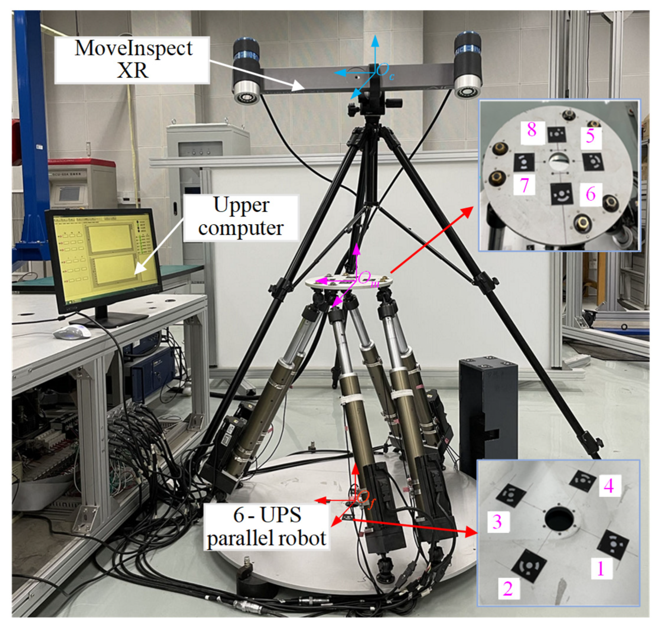
Trajectory error prediction and compensation experiments were conducted on a 6-UPS parallel robot, encompassing a comprehensive experimental framework of trajectory measurement, error prediction, and error compensation. Figure 6 illustrated the established pose measurement system for the six-degree-of-freedom parallel robot. This system is constructed based on the MoveInspect XR 3D optical measurement system from Hexagon, which achieves a single-point measurement accuracy of 5 μm + 10 μm/m within a 2600 mm field of view.
The measurement procedure is as follows: Firstly, four encoded targets are securely affixed to the surfaces of the movable platform and fixed base, respectively. The spatial positions of these targets are measured and used to fit a spatial circle on both platforms. Subsequently, the coordinate systems Of (fixed base) and Om (movable platform) are established based on the circle centers and target positions, determining the poses of both coordinate systems relative to the camera coordinate system Oc. Finally, the transformation matrices Tf and Tm of coordinate systems Of and Om relative to Oc are calculated. The pose of the movable platform relative to the fixed base can then be determined using Tf and Tm. Detailed computational procedures have been described in Reference [24].
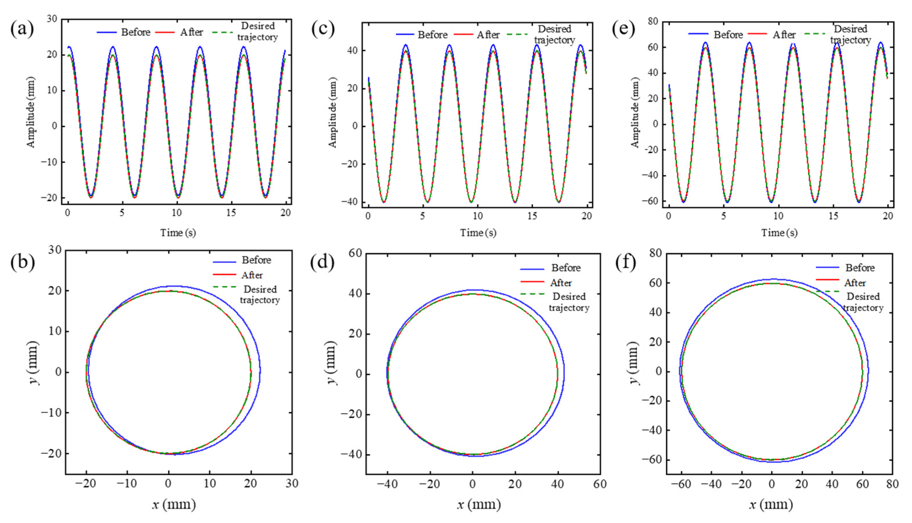
In the experiment, the motion frequency of the parallel robot was set to 0.1 Hz, while the sampling frequency of the 6-DOF measurement system was configured at 40 times the measured motion frequency, i.e., 4 Hz. This sampling frequency adheres to the engineering practice of using at least 10 times the signal frequency for dynamic measurements, thereby ensuring the integrity of the captured data. Other experimental settings remained consistent with the simulation parameters. Figure 7 displayed the sinusoidal and circular trajectories of the 6-UPS parallel robot before and after compensation. A direct comparison reveals that the compensated trajectories exhibit markedly improved conformance to the desired paths for all tested amplitudes and motion types. The proposed method effectively mitigates the predominant error components, notably the amplitude attenuation in sinusoidal motions and the elliptical distortion in circular motions, as visually evidenced by the close overlap between the compensated and desired trajectories. These qualitative results provide clear visual validation of the compensation efficacy, preceding the quantitative analyses that follow.
Table 5 presented a comparative performance evaluation of the CNN-GRU and GRU models in predicting the actual trajectory errors of the parallel robot. The results demonstrate that the CNN-GRU model achieves lower values for both RMSE and MAE compared to the GRU model, indicating its superior predictive performance for trajectory errors. Furthermore, as the trajectory amplitude increases, the predictive performance of the GRU model degrades significantly, whereas the CNN-GRU model maintains relatively stable performance. This robustness was attributed to the CNN’s ability to effectively mitigate noise interference, thereby yielding more reliable predictions. Table 6 summarized the maximum AE and MAE before and after compensation. Following error compensation, the MAEs of the sinusoidal trajectory amplitudes were reduced from 1.4921 mm, 1.5212 mm, and 1.8820 mm to 0.0295 mm, 0.0400 mm, and 0.0544 mm, respectively. Similarly, the MAEs of the circular trajectory amplitudes decreased from 0.4001 mm, 0.4012 mm, and 0.4029 mm to 0.0326 mm, 0.0499 mm, and 0.0326 mm, respectively. These results provided comprehensive validation that the proposed method effectively enhances the trajectory accuracy of the parallel robot.

5. Conclusions

This study presents a deep learning-based method for trajectory error prediction and compensation in parallel robots, enabling accurate forecasting of trajectory errors and their effective correction. By developing a hybrid CNN-GRU network architecture that integrates convolutional and recurrent neural networks, precise prediction of the parallel robot’s trajectory errors is achieved. The model’s key strength lies in its ability to capture complex spatiotemporal dependencies in dynamic trajectories, outperforming conventional methods that are limited to static pose error compensation. Through direct modification of the commanded trajectory at the controller level, dual compensation for both amplitude and offset components of the trajectory error is implemented, significantly enhancing motion trajectory performance. This dual-loop strategy directly addresses the fundamental components of periodic trajectory errors, leading to a transformative improvement in accuracy. Experimental validation on a 6-UPS parallel robot confirms the effectiveness of the proposed approach, demonstrating approximately 90% improvement in accuracy for both sinusoidal and circular trajectories after error compensation. Future work will focus on interpretability analysis of deep learning-based pose and trajectory error prediction, exploring applications of interpretable prediction in fault diagnosis for parallel robots, as well as extensions to other platforms and adaptive learning.

Author Contributions

Conceptualization, Z.L.; Methodology, Z.Z.; Software, Z.Z. and H.H.; Validation, Z.Z.; Formal analysis, Z.L. and C.C.; Investigation, Z.Z.; Resources, C.C. and Y.C.; Data curation, Z.L., H.H. and Y.C.; Writing—original draft, Z.Z.; Writing—review & editing, R.W.; Visualization, C.C.; Supervision, H.H. and Y.C.; Project administration, S.L. All authors have read and agreed to the published version of the manuscript.

Funding

This research was funded by National Key R&D Program of China (No. 2021YFF0600103).

Data Availability Statement

The data presented in this study are available from the corresponding authors upon request. The restriction is due to privacy considerations, since the dataset was privately established and is not open to the public.

Conflicts of Interest

The authors declare no conflict of interest.

References

  1. Zhang, C.; Zhang, L. Kinematics analysis and workspace investigation of a novel 2-DOF parallel manipulator applied in vehicle driving simulator. Robot. Comput. Integr. Manuf. 2013, 29, 113–120. [Google Scholar] [CrossRef]
  2. Huang, P.; Wang, J.; Wang, L.; Yao, R. Identification of structure errors of 3-PRS-XY mechanism with Regularization method. Mech. Mach. Theory 2011, 46, 927–944. [Google Scholar] [CrossRef]
  3. Huang, T.; Zhao, D.; Yin, F.; Tian, W.; Chetwynd, D.G. Kinematic calibration of a 6-DOF hybrid robot by considering multicollinearity in the identification Jacobian. Mech. Mach. Theory 2019, 131, 371–384. [Google Scholar] [CrossRef]
  4. Sun, T.; Song, Y.; Dong, G.; Lian, B.; Liu, J. Optimal design of a parallel mechanism with three rotational degrees of freedom. Robot. Comput. Integr. Manuf. 2012, 28, 500–508. [Google Scholar] [CrossRef]
  5. Song, Y.; Zhang, J.; Lian, B.; Sun, T. Kinematic calibration of a 5-DoF parallel kinematic machine. Precis. Eng. 2016, 45, 242–261. [Google Scholar] [CrossRef]
  6. Zheng, C.; An, Y.; Wang, Z.; Wu, H.; Qin, X.; Eynard, B.; Zhang, Y. Hybrid offline programming method for robotic welding systems. Robot. Comput. Integr. Manuf. 2022, 73, 102238. [Google Scholar] [CrossRef]
  7. Gonzalez, M.K.; Theissen, N.A.; Barrios, A.; Archenti, A. Online compliance error compensation system for industrial manipulators in contact applications. Robot. Comput. Integr. Manuf. 2022, 76, 102305. [Google Scholar] [CrossRef]
  8. Klimchik, A.; Caro, S.; Pashkevich, A. Optimal pose selection for calibration of planar anthropomorphic manipulators. Precis. Eng. 2015, 40, 214–229. [Google Scholar] [CrossRef]
  9. Saund, B.; De, V.R. High Accuracy Articulated Robots with CNC Control Systems. SAE Int. J. Aerosp. 2013, 6, 780–784. [Google Scholar] [CrossRef]
  10. Chen, D.; Yuan, P.; Wang, T.; Cai, Y.; Xue, L. A Compensation Method for Enhancing Aviation Drilling Robot Accuracy Based on Co-Kriging. Int. J. Precis. Eng. Manuf. 2018, 19, 1133–1142. [Google Scholar] [CrossRef]
  11. Wang, W.; Guo, Q.; Yang, Z.; Jiang, Y.; Xu, J. A state-of-the-art review on robotic milling of complex parts with high efficiency and precision. Robot. Comput. Integr. Manuf. 2023, 79, 102436. [Google Scholar] [CrossRef]
  12. Qiang, H.; Xu, D.; Feng, X. Stewart parallel manipulator kinematic calibration based on the normalized identification Jacobian choosing measurement configurations. Opt. Precis. Eng. 2020, 28, 1546–1557. [Google Scholar] [CrossRef]
  13. He, Z.; Song, Y.; Lian, B.; Sun, T. Kinematic Calibration of a 6-DoF Parallel Manipulator with Random and Less Measurements. IEEE Trans. Instrum. Meas. 2023, 72, 7500912. [Google Scholar] [CrossRef]
  14. Fu, L.; Yang, M.; Liu, Z.; Tao, M.; Cai, C.; Huang, H. Stereo vision-based Kinematic calibration method for the Stewart platforms. Opt. Express 2022, 30, 47059–47069. [Google Scholar] [CrossRef]
  15. Alici, G.; Jagielski, R.; Ahmet Sekerciolu, Y.; Shirinzadeh, B. Prediction of geometric errors of robot manipulators with Particle Swarm Optimisation method. Robot. Auton. Syst. 2006, 54, 956–966. [Google Scholar] [CrossRef]
  16. Hu, J.; Hua, F.; Tian, W. Robot Positioning Error Compensation Method Based on Deep Neural Network. In Proceedings of the 2020 4th International Conference on Control Engineering and Artificial Intelligence, Singapore, 17–19 January 2020; Journal of Physics Conference Series. Volume 1487, p. 012045. [Google Scholar]
  17. Dolinsky, J.U.; Jenkinson, I.D.; Colquhoun, G.J. Application of genetic programming to the calibration of industrial robots. Comput. Ind. 2007, 58, 255–264. [Google Scholar] [CrossRef]
  18. Zhou, W.; Liao, W.; Tian, W. Theory and experiment of industrial robot accuracy compensation method based on spatial interpolation. Jixie Gongcheng Xuebao J. Mech. Eng. 2013, 49, 42–48. [Google Scholar] [CrossRef]
  19. Li, B.; Tian, W.; Zhang, C.; Hua, F.; Cui, G.; Li, Y. Positioning error compensation of an industrial robot using neural networks and experimental study. Chin. J. Aeronaut. 2022, 35, 346–360. [Google Scholar] [CrossRef]
  20. Yu, D. A new pose accuracy compensation method for parallel manipulators based on hybrid artificial neural network. Neural Comput. Appl. 2021, 33, 909–923. [Google Scholar] [CrossRef]
  21. Zhu, X.; Liu, Z.; Cai, C.; Yang, M.; Zhang, H.; Fu, L.; Zhang, J. Deep learning-based predicting and compensating method for the pose deviations of parallel robots. Comput. Ind. Eng. 2024, 191, 110179. [Google Scholar] [CrossRef]
  22. Zhu, X.; Zhang, H.; Liu, Z.; Cai, C.; Fu, L.; Yang, M.; Chen, H. Deep learning-based interpretable prediction and compensation method for improving pose accuracy of parallel robots. Expert Syst. Appl. 2025, 268, 126289. [Google Scholar] [CrossRef]
  23. Stewart, D. A Platform with Six Degrees of Freedom (Reprinted from vol 180, 1965). Proc. Inst. Mech. Eng. 2009, 223, 266–273. [Google Scholar] [CrossRef]
  24. Fu, L.; Liu, Z.; Cai, C.; Tao, M.; Yang, M.; Huang, H. Joint space-based optimal measurement configuration determination method for Stewart platform kinematics calibration. Measurement 2023, 211, 112646. [Google Scholar] [CrossRef]
  25. Toquica, J.S.; Oliveira, P.S.; Souza, W.S.R.; Motta, J.M.S.T.; Borges, D.L. An analytical and a Deep Learning model for solving the inverse kinematic problem of an industrial parallel robot. Comput. Ind. Eng. 2021, 151, 106682. [Google Scholar] [CrossRef]
  26. Petraova, I.; Karban, P. Solving evolutionary problems using recurrent neural networks. J. Comput. Appl. Math. 2023, 426, 115091. [Google Scholar] [CrossRef]
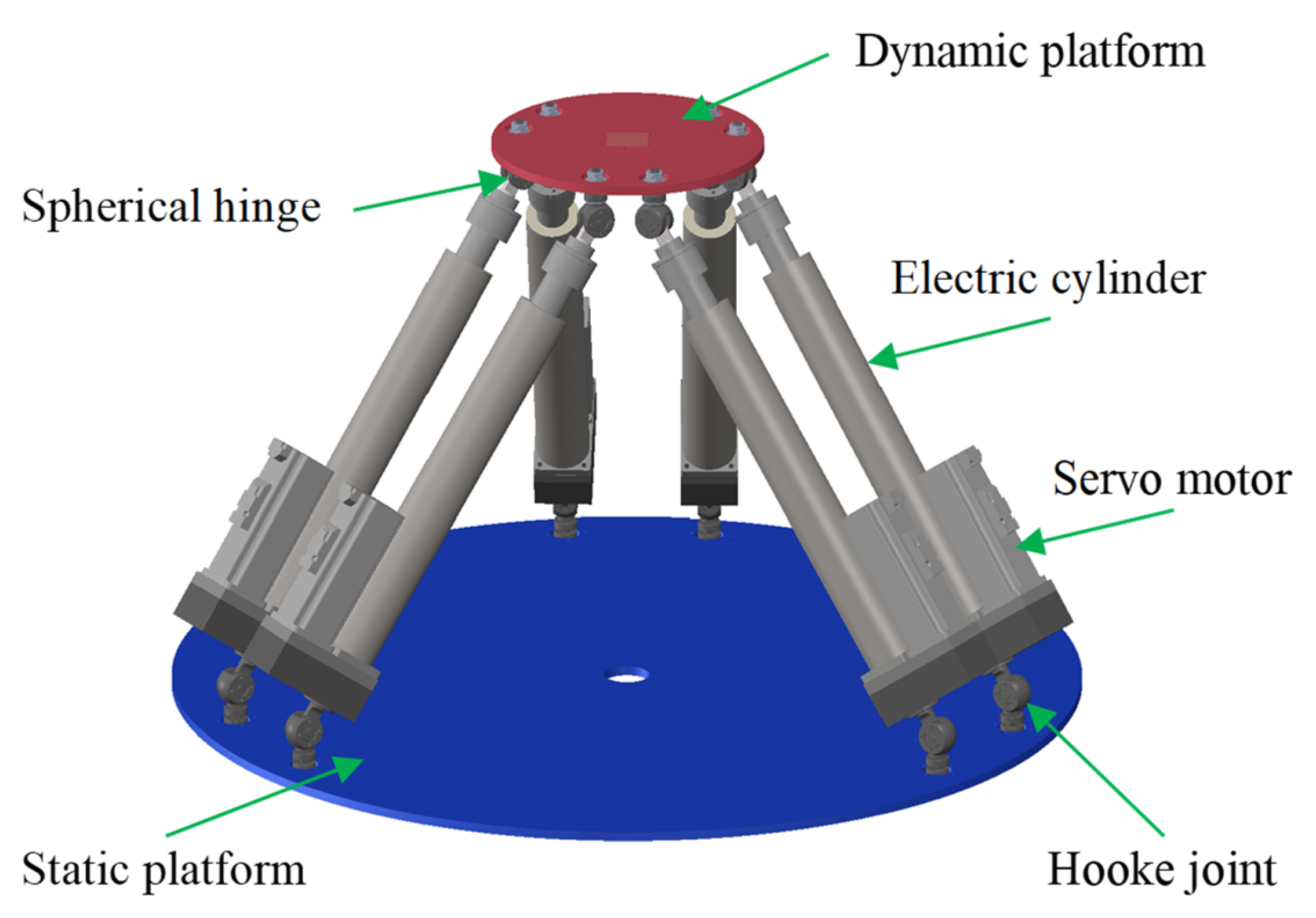
Figure 1. The 3D schematic of the 6-UPS parallel robot.
Electronics 14 04752 g001
Figure 2. Schematic of the parallel robot: (a) kinematic diagram; (b) limb vector loop.
Electronics 14 04752 g002
Figure 3. Architecture of the CNN-GRU model.
Electronics 14 04752 g003
Figure 4. Simulation Data Generation and Model Training.
Electronics 14 04752 g004
Figure 5. Exemplary trajectory errors of the parallel robot: (a) the desired versus actual trajectory; (b) the trajectory errors.
Electronics 14 04752 g005
Figure 6. The established experimental system.
Electronics 14 04752 g006
Figure 7. Trajectory error compensation results: (a) 20 mm sinusoidal; (b) 20 mm circular; (c) 40 mm sinusoidal; (d) 40 mm circular; (e) 60 mm sinusoidal; (f) 60 mm circular.
Electronics 14 04752 g007
Table 1. Geometric parameter errors (mm).
LimbΔaixΔaiyΔaizΔbixΔbiyΔbizΔli
10.5959−0.87240.0221−3.2560−0.3268−1.3285−0.1221
2−0.8934−0.79480.7351−8.72410.62291.7698−1.7148
3−0.9396−0.28881.8452−1.1413−2.7663−0.20121.6943
40.5393−0.44551.60123.4204−4.1089−0.44530.8355
50.17250.62753.14310.93813.58742.5500−0.8717
6−0.2835−1.0608−2.02311.22703.2504−0.2171−2.1385
Table 2. Hyperparameter configuration of the CNN-GRU model.
HyperparameterSize/QuantityHyperparameterValue/Function
Convolutional Kernel Size3 × 1, 3 × 1Number of GRU6
Number of Convolutional Kernels6, 3OptimizerAdam
Batch Size32Loss FunctionMAE
Number of Training Epochs500Decay Steps400
Initial Learning Rate0.01Decay Rate0.1
Table 3. Predictive performance evaluation of the models.
Amplitude/mmCNN-GRUGRU
RMSEMAERMSEMAE
200.00250.00300.00300.0037
400.00270.00320.00400.0049
600.00280.00320.00490.0060
Table 4. Trajectory errors before and after compensation.
Amplitude/RadiusBefore Compensation (mm)After Compensation (mm)
Max. AEMAEMax. AEMAE
Ax = 200.78220.68870.00590.0024
Ax = 400.86990.68880.00580.0025
Ax = 600.95790.68890.00640.0026
rxoy = 200.46820.40010.03160.0164
rxoy = 400.53230.40120.05450.0319
rxoy = 600.59740.40290.08140.0475
Table 5. Comparative performance evaluation of the models.
Amplitude/mmCNN-GRUGRU
RMSEMAERMSEMAE
200.01950.01670.01720.0181
400.01960.01590.02130.0255
600.03590.02990.04780.0451
Table 6. Trajectory errors before and after compensation.
Amplitude/
Radius
Before Compensation (mm)After Compensation (mm)
Max. AEMAEMax. AEMAE
Ax = 202.31701.49210.07300.0295
Ax = 403.15791.52120.08220.0400
Ax = 604.03671.88200.06270.0544
rxoy = 201.69810.97570.06520.0326
rxoy = 402.48191.20510.09870.0499
rxoy = 603.25551.61800.09790.0389
Disclaimer/Publisher’s Note: The statements, opinions and data contained in all publications are solely those of the individual author(s) and contributor(s) and not of MDPI and/or the editor(s). MDPI and/or the editor(s) disclaim responsibility for any injury to people or property resulting from any ideas, methods, instructions or products referred to in the content.