Selective Learnable Discounting in Deep Evidential Semantic Mapping

Abstract

In autonomous driving and mobile robotics applications, constructing accurate and reliable three-dimensional semantic maps poses significant challenges in resolving conflicts and uncertainties among multi-frame observations in complex environments. Traditional deterministic fusion methods struggle to effectively quantify and process uncertainties in observations, while existing evidential deep learning approaches, despite providing uncertainty modeling frameworks, still exhibit notable limitations when dealing with spatially varying observation quality. This paper proposes a selective learnable discounting method for deep evidential semantic mapping that introduces a lightweight selective $\alpha$-Net network based on the EvSemMap framework proposed by Kim and Seo. The network can adaptively detect noisy regions and predict pixel-level discounting coefficients based on input image features. Unlike traditional global discounting strategies, this work employs a theoretically principled scaling discounting formula, ${\widehat{e}}_k\left(x\right)=\alpha \left(x\right)·e_k\left(x\right)$, that conforms to Dempster–Shafer theory, implementing a selective adjustment mechanism that reduces evidence reliability only in noisy regions while preserving original evidence strength in clean regions. Theoretical proofs verify three core properties of the proposed method: evidence discounting under preservation (ensuring no loss of classification accuracy), valid uncertainty redistribution validity (effectively suppressing overconfidence in noisy regions), and optimality of discount coefficients (achieving the matching of the theoretical optimal solution of ${\alpha }^{*}\left(x\right)=1-N\left(X\right)$). Experimental results demonstrate that the method achieves a 43.1% improvement in Expected Calibration Error (ECE) for noisy regions and a 75.4% improvement overall, with $\alpha$-Net attaining an IoU of 1.0 with noise masks on the constructed synthetic dataset—which includes common real-scenario noise types (e.g., motion blur, abnormal illumination, and sensor noise) and where RGB features correlate with observation quality—thereby fully realizing the selective discounting design objective. Combined with additional optimization via temperature calibration techniques, this method provides an effective uncertainty management solution for deep evidential semantic mapping in complex scenarios.

1. Introduction

With the rapid development of artificial intelligence technologies, the autonomous navigation capabilities of self-driving vehicles and mobile robots in complex environments have become a focal point for both academia and industry. Constructing accurate and reliable three-dimensional semantic maps, as one of the core technologies for achieving advanced autonomous navigation, requires not only accurate identification of various semantic objects in the environment but also the effective handling of conflicts and uncertainties in multi-frame observation information from different time points and viewing angles [1,2]. In real robotic operating environments, the presence of sensor noise, illumination changes, motion blur, occlusion, and other factors makes observations from different frames often contain contradictory information. How to scientifically quantify and process these uncertainties has become a critical challenge in the field of semantic mapping [3,4].

Traditional semantic mapping methods primarily rely on deterministic fusion strategies, such as simple majority voting mechanisms or weighted averaging methods based on preset confidence levels [5,6], and hybrid models like the Feature Cross-Layer Interaction Hybrid Model (FCIHMRT) [7]. While these methods can achieve good results under ideal conditions, when facing complex real environments, they often lead to significant degradation in map quality due to their lack of accurate modeling and quantification capabilities for observation uncertainties [8]. In recent years, with the flourishing development of deep learning technology, neural network-based semantic segmentation methods have achieved significant progress in accuracy [9,10]. However, these methods typically only provide point estimates and are limited in their ability to quantify prediction uncertainties, which is problematic in safety-critical robotic applications [11].

To address the aforementioned problems, evidential deep learning (EDL) has emerged as a novel uncertainty quantification framework [12]. EDL directly models epistemic uncertainty by predicting parameters of Dirichlet distributions, avoiding the computational burden of complex sampling or variational inference required by traditional Bayesian methods [13]. Sensoy et al. [12] first proposed the basic framework of EDL, followed by Amini et al. [14], who applied it to semantic segmentation tasks in autonomous driving, demonstrating its superiority especially in the presence of out-of-distribution (OOD) inputs. Building on this foundation, Kim and Seo [15] proposed the EvSemMap method, which merges EDL with Dempster–Shafer (DS) theory, and applied it to the field of semantic mapping, predicting pixel-level evidence vectors through evidence generation networks and utilizing DS theory’s combination rules for multi-frame evidence fusion.

Despite the theoretical innovation of the EvSemMap method, it still exhibits noteworthy limitations in practical applications. The method applies the same processing strategy to all observations, lacking the capability to adaptively modulate discounting based on observation quality, which leads to performance degradation in complex scenarios with substantial sensor noise or low-quality inputs [16]. Furthermore, existing evidence discounting mechanisms typically employ globally uniform discounting coefficients, which are unable to make fine-grained adjustments for quality differences across image regions [17].

Addressing these challenges, this paper proposes a selective learnable discounting method for deep evidential semantic mapping. The core innovation of this method lies in a design of a lightweight selective $\alpha$-Net network that can automatically detect noisy regions and predict pixel-level discounting coefficients based on RGB image features. Compared with traditional global discounting strategies, this method achieves spatially adaptive selective discounting, preserving original evidence strength in clean regions ($\alpha \approx 1$) while significantly reducing evidence reliability in noisy regions or low-quality regions ($\alpha \approx 0$). Simultaneously, this work employs a theoretically principled scaling discounting formula that conforms to Dempster–Shafer (DS) theory, ensuring theoretical consistency and robustness of the method.

The main contributions of this paper can be summarized as follows: First, we propose the concept and implementation of selective discounting, overcoming the limitations of traditional global discounting and achieving fine-grained evidence adjustment based on observation quality. Second, we design a lightweight $\alpha$-Net network architecture that achieves high-precision noisy-region identification while ensuring computational efficiency. Third, we prove three core theoretical properties of the method: evidence order preservation, valid uncertainty redistribution, and optimal discount coefficient; we also derive a formal algorithm, ensuring mathematical rigor and experimental reproducibility. Fourth, we employ a theoretically principled scaling discounting formula, thereby reinforcing the mathematical rigor of the method. Finally, we comprehensively validate the method through experiments, particularly demonstrating significant improvements in confidence calibration and robustness under noise.

2. Related Work

2.1. Semantic Mapping and Uncertainty Handling

Semantic mapping, as an important component of robotic perception systems, aims to construct environment representations containing rich semantic information, providing a foundation for high-level robot cognition and decision making [18]. Early semantic mapping research primarily focused on combining traditional geometric SLAM with semantic segmentation techniques for enhanced environment representation. Salas-Moreno et al. [19] proposed the SLAM++ system, achieving more compact and meaningful map representations by modeling environments as collections of semantic objects. McCormac et al. [20] developed the SemanticFusion system, utilizing CNNs for real-time semantic segmentation and constructing semantic maps via probabilistic fusion.

With the development of deep learning methods, neural network-based semantic mapping approaches have gradually become mainstream. Rosinol et al. [21] proposed the Kimera system, achieving real-time metric–semantic SLAM capable of constructing mesh maps containing semantic information. Hughes et al. [22] further developed the concept of 3D scene graphs, extending semantic mapping to higher-level scene understanding. However, most of these methods rely on deterministic fusion strategies and are limited in their ability to manage observational uncertainties.

Beyond deterministic and deep learning-based semantic mapping, a range of non-evidential frameworks have been explored for uncertainty modeling and sensor fusion discounting, yet they exhibit notable limitations. Bayesian deep learning methods, such as Bayesian CNNs [23], model epistemic uncertainty via Monte Carlo dropout, enabling stochastic uncertainty estimation without complex variational inference. However, these methods suffer from high computational overhead in multi-frame fusion—repeated forward passes are required to sample posterior distributions, making them impractical for real-time robotic applications like autonomous driving. Kalman filter variants (e.g., Extended Kalman Filter and Unscented Kalman Filter), a classical sensor fusion paradigm, have long been used for uncertainty propagation in geometric SLAM [1]. They quantify aleatoric uncertainty (e.g., sensor noise) via covariance matrices but fail to handle epistemic uncertainty (e.g., ambiguous semantic labels) or spatially varying observation quality—critical gaps in complex environments with uneven sensor performance. Gaussian Process (GP)-based mapping models uncertainty in semantic predictions but scales poorly to large-scale 3D environments due to O(n³) complexity in kernel computations, restricting its application in large robotic navigation scenarios. Meanwhile, deterministic uncertainty estimation methods like temperature calibration and Platt scaling [24] adjust confidence scores to align with empirical accuracy. These methods are computationally efficient but lack spatial context integration—they cannot distinguish noisy regions from clean regions in images, nor propagate uncertainty across multi-frame observations, limiting their utility in dynamic semantic mapping.

In recent years, researchers have begun to focus on uncertainty quantification issues in semantic mapping. Gawel et al. [25] proposed probability-based semantic mapping methods that improve map quality by modeling prediction uncertainties. Stachniss et al. [26] emphasized in their survey the importance of uncertainty handling in robotic perception. Valada et al. [27] proposed multi-modal deep learning approaches that reduce uncertainty by fusing information from multiple sensors. These works have laid important foundations for our research.

2.2. Evidential Deep Learning Theory and Applications

Evidential deep learning (EDL), as an emerging single-forward-pass uncertainty quantification framework, has rigorous theoretical foundations traceable to Dempster–Shafer evidence theory [28,29]. Sensoy et al. [12] introduced the EDL framework, which directly models epistemic uncertainty by predicting parameters of Dirichlet distributions. The core concept is to interpret neural network outputs as evidence masses supporting different categories and then construct belief distributions (and uncertainty mass) based on this evidence.

An important advantage of EDL methods is their ability to separate epistemic from aleatoric uncertainties. Epistemic uncertainty arises from insufficient model knowledge or under-sampling and decreases with more or diversified training data. Aleatoric uncertainty, conversely, reflects inherent observation noise or ambiguity in input data and cannot be reduced via additional data [30]. This distinction is of great significance for robotic applications, as it helps systems identify when more observational data are needed.

This advantage of EDL distinguishes it from other non-evidential uncertainty estimation approaches commonly used in robotic perception. Ensemble-based methods [31] estimate uncertainty via diverse model predictions, which improves robustness but requires training multiple models—resulting in high memory and latency costs that are unsuitable for resource-constrained robotic platforms (e.g., small mobile robots). Contrastive learning-based uncertainty methods [26] leverage feature similarity to identify uncertain regions, but they rely on labeled data to construct contrastive pairs, limiting their applicability to unannotated or noisy datasets (e.g., disaster response scenarios with incomplete labels). In contrast, EDL achieves uncertainty quantification with a single forward pass, avoiding the overhead of ensembles or labeled contrastive pairs while explicitly modeling “ignorance” (e.g., out-of-distribution inputs)—a key requirement for safety-critical robotic tasks.

Wilson et al. [32] applied EDL to semantic segmentation tasks in autonomous driving, demonstrating enhanced robustness against out-of-distribution (OOD) inputs. Jiang et al. [33] proposed improved EDL loss functions, enhancing uncertainty estimation accuracy by introducing KL divergence regularization terms, which help suppress overconfidence in uncertain regions. Kumar et al. [34] further studied EDL applications in medical image segmentation, showcasing its potential in handling label noise and annotation uncertainties. More recently, works such as R-EDL Chen et al. [35,36] revisit non-essential settings in standard EDL (e.g., fixed prior weights and variance-minimization terms), improving calibration and reducing overconfidence [37,38].

However, many existing EDL approaches still suffer from limitations when observation quality varies spatially. They typically employ globally uniform evidence processing or discounting and are unable to adapt to per-pixel or region-level quality differences across images. Moreover, few existing works provide theoretical guarantees that discounting mechanisms align with DS combination rules under such non-uniform evidence suppression. The selective learnable discounting mechanism proposed in this paper is specifically designed to fill this gap.

2.3. Applications of Dempster–Shafer Theory in Computer Vision

Dempster–Shafer (DS) theory, as a well-established mathematical framework for handling incomplete and uncertain information, has seen extensive use in computer vision [39]. The core concepts of this theory include Basic Probability Assignment (BPA), Belief Function, and Plausibility Function, which collectively provide a rigorous mathematical foundation for uncertainty representation and reasoning [40].

In the domain of multi-sensor fusion, DS theory is widely used for fusing evidence from heterogeneous sources. Bloch et al. [41] provided a systematic survey of DS theory in image processing, including image segmentation, object detection, and classification. Denoeux et al. [42] applied DS theory to pattern recognition by combining outputs from multiple classifiers via evidence combination rules to improve classification reliability.

In recent years, with the development of deep learning and its success in perception tasks, researchers have begun exploring hybrid methods that combine DS theory with neural networks. Tong et al. [24] proposed deep fusion networks grounded in DS theory for multi-modal emotion recognition, demonstrating how evidence combination under DS can improve robustness when modalities conflict. Deregnaucourt et al. [31] proposed the ECoLaF method, using conflict-aware measures to guide multi-modal evidence fusion, which offers useful inspiration for our work in terms of managing conflicting evidence.

The discounting operation in DS theory is a central mechanism for handling unreliable low-quality evidence. Shafer [29] defined standard discounting operations in the original theory; however, they are non-differentiable and thus not directly compatible with gradient-based deep learning frameworks. In recent years, some research has attempted to introduce learnable or parametric discounting mechanisms into deep learning; however, most still rely on global discount rates or uniform discounting, lacking spatial or regional adaptivity [43].

2.4. EvSemMap Method and Its Limitations

The EvSemMap method, proposed by Kim and Seo [15], is a pioneering work that integrates evidential deep learning (EDL) with DS theory in the semantic mapping domain. This method predicts pixel-level evidence vectors via evidence generation networks, employs Dempster combination rules for multi-frame fusion, and introduces conflict measures as map quality evaluation metrics grounded in evidence conflict theory. EvSemMap’s main contributions include establishing rigorous conversion mechanisms from raw evidence to Basic Probability Assignments (BPAs), designing evidence fusion processes explicitly tailored to semantic map construction, and proposing conflict-based metrics for evaluating map quality.

However, EvSemMap exhibits several critical limitations in real-world or complex scenarios. First, the method applies a uniform processing strategy to all observations, lacking the capacity to adapt discounting or evidence weighting based on observation quality metrics. In complex scenarios with substantial sensor noise, occlusions, illumination variation, or low-quality inputs, this “one-size-fits-all” processing strategy often leads to noticeable performance degradation in map accuracy and reliability [44]. Second, existing evidence discounting mechanisms typically use globally uniform discount factors or coefficients, making them unable to perform fine-grained per-pixel or region-level adjustments for spatial quality variations within images [45].

Furthermore, EvSemMap has issues in its theoretical implementation. For instance, the linear combination discounting formula it employs is not proven to be consistent with DS theory’s axioms and may distort relative ordering or relationships among evidence sources [46].

These limitations motivate the development of an improved selective learnable discounting method, which adapts evidence discounting spatially, preserves evidence integrity in high-quality observations, and maintains theoretical consistency.

3. Methodology

3.1. Problem Modeling and Theoretical Foundation

In mobile robotic semantic mapping tasks, the system processes sequences of RGB-D observations from different time points. At time t, the robot obtains an RGB image $I_t\in {\mathbb{R}}^{H\times W\times 3}$ and a corresponding depth map $D_t\in {\mathbb{R}}^{H\times W}$, along with the camera pose $T_t\in SE\left(3\right)$. The goal of semantic mapping is to construct a global three-dimensional semantic map M, where each voxel v in the map is associated with a semantic label distribution (i.e., a probability distribution over semantic classes for that voxel).

Consider a semantic category set $\mathsf{\Omega }=\{l_1,l_2,\dots ,l_K\}$ with K total categories. For each pixel $x=(u,v)$ in the image, the evidential segmentation network (denoted by $f_{\mathrm{evid}}$) predicts an evidence vector:

$$e\left(x\right)=f_{\mathrm{evid}}(I_t;x)={[e_1\left(x\right),e_2\left(x\right),\dots ,e_K\left(x\right)]}^T$$

(1)

Here $e_k\left(x\right)\ge 0$ represents the evidence strength supporting the hypothesis that pixel x belongs to category $l_k$. Intuitively, $e_k\left(x\right)$ can be viewed as the amount of support or “evidence” that the network has accumulated for class $l_k$ at pixel x, with larger values indicating higher confidence in that class hypothesis.

Under the Dempster–Shafer theory (DST) framework, the evidence vector $e\left(x\right)$ is converted into a Basic Probability Assignment (BPA) over the K classes plus an uncertainty mass. Let

$$S\left(x\right)=\sum _{k=1}^K{e}_k\left(x\right)+K$$

(2)

be the total evidence strength including a prior of 1 for each class (the $+K$ term). Then we define the belief mass assigned to class ${\ell }_k$ and the uncertainty mass as

$$b_k\left(x\right)={\displaystyle \frac{e_k\left(x\right)}{S\left(x\right)}},u\left(x\right)={\displaystyle \frac{K}{S\left(x\right)}}$$

(3)

By construction, $b_k\left(x\right)\ge 0$, $u\left(x\right)\ge 0$, and ${\sum }_{k=1}^K{b}_k\left(x\right)+u\left(x\right)=1$. The belief masses $\left\{b_k\left(x\right)\right\}$ represent the committed probability mass for each class (based on the evidence), while $u\left(x\right)$ represents the remaining uncommitted mass (due to insufficient or conflicting evidence, i.e., epistemic uncertainty). Finally, to obtain a single-point class prediction from this evidential distribution, we employ the subjective logic opinion pooling method. Assuming a neutral prior (no bias to any class), the final class probability for ${\ell }_k$ is given by distributing the uncertainty mass equally among all classes:

$$p_k\left(x\right)=b_k\left(x\right)+{\displaystyle \frac{u\left(x\right)}{K}}$$

(4)

Equivalently, $p_k\left(x\right)={\displaystyle \frac{e_k\left(x\right)+1}{S\left(x\right)}}$, which is exactly the expected probability of class ${\ell }_k$ under a Dirichlet distribution parameterized by ${\alpha }_k=e_k\left(x\right)+1$. This modeling approach explicitly represents and quantifies prediction uncertainty for each pixel, providing a rigorous theoretical foundation for subsequent multi-frame evidence fusion and quality assessment in the mapping system.

3.2. Selective Learnable Discounting Mechanism

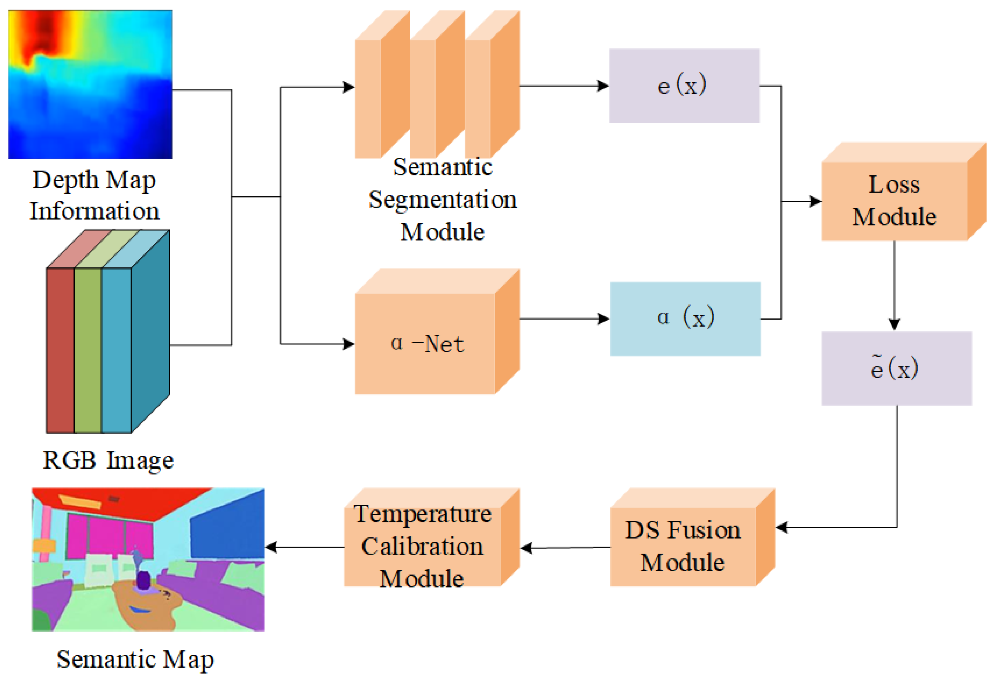
The flowchart in Figure 1 outlines the holistic framework of the proposed selective learnable discounting approach for deep evidential semantic mapping, which is developed based on the EvSemMap framework proposed by Kim and Seo [15] to address the limitation of spatially invariant observation quality handling in existing methods. As depicted, the system takes RGB images (a fundamental input in mobile robotic semantic mapping tasks) as the starting point. First, it extracts pixel-level RGB feature vectors $f_{\mathrm{RGB}}\left(x\right)\in {\mathbb{R}}^3$—these features encode local image attributes (e.g., normalized color intensity) that correlate with observation quality, such as distinguishing well-exposed clean regions from dark or blurred noisy regions. These RGB features are input to the lightweight selective $\alpha$-Net, the core module of this work. Designed with computational efficiency and interpretability in mind, $\alpha$-Net adopts a simple logistic regression structure (with learnable parameters $\mathit{w}\in {\mathbb{R}}^3$ and $b\in \mathbb{R}$) to output a pixel-wise discount coefficient map $\left\{\alpha \right(x\left)\right\}$. Its key function is to adaptively identify noisy regions (e.g., motion-blurred areas, extreme illumination regions, or regions with severe sensor noise) and assign corresponding $\alpha \left(x\right)$ values: in clean regions where observations are reliable, $\alpha \left(x\right)\approx 1$ to retain the original evidence strength; in noisy regions with unreliable observations, $\alpha \left(x\right)\approx 0$ to reduce evidence influence. The predicted $\alpha \left(x\right)$ is then applied to the original evidence vector $e\left(x\right)$ (output by the evidential segmentation network $f_{\mathrm{evid}}$) via the scaling discounting formula ${\widehat{e}}_k\left(x\right)=\alpha \left(x\right)·e_k\left(x\right)$—a formulation that strictly complies with Dempster–Shafer (DS) theory, ensuring theoretical consistency. After discounting, the processed evidence $\widehat{e}\left(x\right)$ undergoes temperature calibration to optimize confidence distribution, followed by multi-frame evidence fusion using DS combination rules to construct the final 3D semantic map. Additionally, the framework integrates a multi-component loss function (including cross-entropy loss for classification accuracy, conflict loss for fusion consistency, regularization loss for $\alpha \left(x\right)$ reasonableness, and total variation smoothness loss for spatial coherence of the discount map) to jointly optimize $\alpha$-Net and the evidential segmentation network, guaranteeing the effectiveness of selective discounting in complex scenarios.

Traditionally, evidential discounting methods in DST use a single, globally uniform discount factor for an entire image or sensor input. This “one-size-fits-all” approach fails to account for spatial variations in observation quality across an image. In real robotic perception scenarios (e.g., an autonomous driving scene), a single camera frame can contain both high-quality, clear regions and low-quality regions corrupted by noise. For instance, an image may have well-exposed areas that yield confident semantic predictions while also containing motion-blurred or overexposed portions that produce unreliable predictions. Applying the same discount factor to all regions is clearly suboptimal, as low-quality regions should be trusted less than high-quality ones.

The selective discounting mechanism proposed in this work is based on a core principle: high-quality observations should retain their original evidence strength, whereas low-quality observations should have their evidence discounted (down-weighted) to reduce their influence on the final decision. To implement this principle, we first define a binary noise mask to identify low-quality regions. Let $N\left(x\right)\in \{0,1\}$ indicate whether pixel x lies in a noise-affected region:

$$N\left(x\right)=\left\{\begin{array}{cc}1,\hfill & \mathrm{if}\mathrm{pixel}x\mathrm{is}\mathrm{in}\mathrm{a}\mathrm{noise}\text{-}\mathrm{corrupted}\mathrm{region},\hfill \\ 0,\hfill & \mathrm{if}\mathrm{pixel}x\mathrm{is}\mathrm{in}\mathrm{a}\mathrm{clean}\mathrm{region}(\mathrm{no}\mathrm{significant}\mathrm{noise}),\hfill \end{array}\right.$$

(5)

where a noisy region may correspond to phenomena such as motion blur, extreme illumination (glare or shadows), severe sensor noise, or occlusion by foreign objects. These conditions tend to degrade the reliability of the pixel’s semantic evidence. The selective discounting strategy is to adaptively assign each pixel a discount factor $\alpha \left(x\right)$ based on the pixel’s estimated quality: in a clean region $N\left(x\right)=0$, we desire $\alpha \left(x\right)\approx 1$ (retain full trust in the evidence), whereas in a noisy region $N\left(x\right)=1$, we set $\alpha \left(x\right)\approx 0$ (heavily down-weight the unreliable evidence). This adaptive strategy ensures that low-quality observations have a diminished impact on the semantic map, while high-quality observations can contribute at full strength. For example, consider an autonomous driving scenario where part of the camera image is blurred due to rapid motion, while another part is clear. The selective discounting mechanism will assign a small $\alpha \left(x\right)$ to pixels in the blurred region (effectively ignoring their dubious evidence) and $\alpha \left(x\right)\approx 1$ to pixels in the clear region (fully trusting their evidence). This way, the final fused semantic understanding of the scene is not skewed by the noisy observations, improving overall robustness in challenging traffic environments.

To automatically distinguish noisy regions from clear regions and predict appropriate $\alpha \left(x\right)$ values, we design a lightweight learnable module termed selective $\alpha$-Net. This module takes the image (or relevant features of the image) as input and outputs a pixel-wise discount map {$\alpha$(x)} across the image.

$$\alpha \left(x\right)=f_{\alpha }(I_t;x),$$

(6)

where $f_{\alpha }$ denotes the $\alpha$-Net function (a small neural network). In our implementation, $f_{\alpha }$ is realized as a simple logistic regression on raw pixel intensity values for efficiency and interpretability. Specifically, let $f_{\mathrm{RGB}}\left(x\right)\in {\mathbb{R}}^3$ be a 3-dimensional feature vector representing pixel x (e.g., the normalized RGB color of the pixel). The discount factor is predicted by

$$alpha\left(x\right)=\sigma (w^T{f}_{\mathrm{RGB}}\left(x\right)+b)$$

(7)

where $\mathbf{w}\in {\mathbb{R}}^3$ and $b\in \mathbb{R}$ are learnable parameters and $\sigma (·)$ is the sigmoid activation function (ensuring $0<\alpha \left(x\right)<1$). This design uses only a few parameters, is computationally fast, and is interpretable—each weight in $\mathbf{w}$ indicates how the corresponding color channel influences the predicted image quality. High-quality regions (often with normal color exposure and contrast) can be learned to yield $\alpha \approx 1$, whereas known noise patterns (e.g., overly dark or bright pixels, or certain color tints associated with sensor artifacts) can lead to $\alpha \approx 0$. Selective $\alpha$-Net, therefore, provides an efficient, learnable way to realize pixel-level discounting that tailors the evidential trust to local observation conditions.

3.3. Correct Scaling Discounting Formula

The output of $\alpha$-Net is a pixel-wise discount map $\left\{\alpha \right(x\left)\right\}$, where each $\alpha \left(x\right)\in [0,1]$ acts as a discount factor on the local evidential vector. For visualization purposes, we also refer to this $\alpha$-map as a “trust map”, since a larger $\alpha \left(x\right)$ indicates higher trust in the corresponding observation; in the remainder of the paper, we use the terms “discount map”, “$\alpha$-map”, and “trust map” interchangeably to denote this learned reliability field.

In implementing evidence discounting, the choice of how $\alpha \left(x\right)$ is applied to the evidence is critical to both theoretical correctness and practical effectiveness. A seemingly reasonable approach is a linear combination of the original evidence with some default evidence. For example, one might discount evidence by blending it with a neutral “unit evidence” value as follows:

$${\widehat{e}}_k\left(x\right)=\alpha \left(x\right)·e_k\left(x\right)+(1-\alpha \left(x\right))·1$$

(8)

Here the idea is that when $\alpha \left(x\right)=1$ (full trust), the evidence remains ${\tilde{e}}_k=e_k$; when $\alpha \left(x\right)=0$ (no trust), this formula replaces $e_k$ with a unit value (the term 1) for all classes, which yields an uninformative uniform distribution after normalization. However, Equation (8) is fundamentally flawed. Its problems are threefold: (1) it does not conform to the formal definition of evidence discounting in Dempster–Shafer theory, and it introduces an ad hoc unit evidence term; (2) it can distort the relative proportions among the evidence values (adding a constant 1 to each $e_k$ changes their ratios), potentially affecting prediction stability; and (3) it lacks rigorous theoretical justification. In summary, Equation (8) is an improper discounting operation that can produce inconsistent or biased results.

Instead, we adopt a scaling discounting formula that strictly follows Dempster–Shafer theory. In DST, discounting a source of evidence by a factor $\alpha$ means multiplying all the source’s belief masses by $\alpha$ and reallocating the remaining $1-\alpha$ mass to ignorance. We, therefore, apply $\alpha \left(x\right)$ by directly scaling the evidence values:

$${\widehat{e}}_k\left(x\right)=\alpha \left(x\right)·e_k\left(x\right)$$

(9)

This formulation ensures that all specific evidence (for each class ${\ell }_k$) is reduced by the factor $\alpha \left(x\right)$, while the remaining weight $(1-\alpha (x\left)\right)$ effectively goes into increasing the uncertainty. In the DST sense, the masses for concrete hypotheses are multiplied by $\alpha$, and the lost mass $1-\alpha$ is transferred to the ignorance mass (which corresponds to $u\left(x\right)$ in our model). For example, if $\alpha \left(x\right)=0$, then ${\tilde{e}}_k\left(x\right)=0$ for all k, meaning that the observation contributes no class-specific evidence at all—in this extreme, all belief is unassigned, and $\tilde{u}\left(x\right)=1$, indicating total ignorance. Conversely, if $\alpha \left(x\right)=1$, then ${\tilde{e}}_k\left(x\right)=e_k\left(x\right)$ (no discounting), and the uncertainty mass $\tilde{u}\left(x\right)$ remains at its minimum (same as the original $u\left(x\right)$). Partial values $0<\alpha <1$ will proportionally scale down the evidence and implicitly increase the relative uncertainty. In contrast to Equation (8), Equation (9) does not inject any arbitrary “unit evidence”—it simply modulates the strength of the existing evidence, which is the proper DST way to discount.

Scaling discounting (Equation (9)) offers multiple advantages. From a theoretical perspective, it adheres exactly to the mathematical definition of discounting in evidence theory, ensuring that our discounting operation is theoretically sound and consistent with DST. From a practical perspective, scaling maintains the relative relationships among the evidence components—if $e_i\left(x\right)>e_j\left(x\right)$ initially, then ${\tilde{e}}_i\left(x\right)>{\tilde{e}}_j\left(x\right)$ as well (provided $\alpha \left(x\right)>0$)—preserving the rank and thus avoiding unpredictable shifts in the predicted class. Moreover, the extreme cases are intuitive: $\alpha \left(x\right)=0$ implies complete distrust of that pixel’s evidence (all weight goes to uncertainty), while $\alpha \left(x\right)=1$ implies full trust (evidence unchanged). Partial values $0<\alpha \left(x\right)<1$ will proportionally scale down the evidence and implicitly increase the relative uncertainty. From a computational perspective, Equation (9) is simple and differentiable, making it compatible with gradient-based learning and easy to integrate into a deep learning pipeline without additional complexity.

After discounting, the discounted evidence vector $\tilde{\mathbf{e}}\left(x\right)={[{\tilde{e}}_1\left(x\right),\dots ,{\tilde{e}}_K\left(x\right)]}^T$ is processed in the same way as before to produce the final probabilities. We first recompute the total evidence (including the prior) as

$$\tilde{S}\left(x\right)=\sum _{k=1}^K{\tilde{e}}_k\left(x\right)+K$$

(10)

and derive the discounted belief masses ${\tilde{b}}_k\left(x\right)$ and residual uncertainty $\tilde{u}\left(x\right)$:

$${\tilde{b}}_k\left(x\right)={\displaystyle \frac{{\tilde{e}}_k\left(x\right)}{\tilde{S}\left(x\right)}},\tilde{u}\left(x\right)={\displaystyle \frac{K}{\tilde{S}\left(x\right)}}$$

(11)

The final predicted probability for class ${\ell }_k$ after discounting is then

$${\tilde{p}}_k\left(x\right)={\tilde{b}}_k\left(x\right)+{\displaystyle \frac{\tilde{u}\left(x\right)}{K}}$$

(12)

This ensures that the discounted evidence is correctly converted into a probability distribution over classes, just as in Equation (12) for the original evidence. By applying the discount at the evidence level and then propagating it through the subjective logic transformation, we maintain consistency and correctness of the inference process end to end—any down-weighting of unreliable evidence is faithfully reflected in the final class probabilities and ultimately in the fused semantic map.

3.4. Loss Function Design and Optimization Strategy

To train selective $\alpha$-Net and optimize the overall system, we formulate a multi-component loss function that addresses multiple objectives. In particular, the training loss is designed to ensure high classification accuracy, encourage the discounting network to learn meaningful (non-trivial) $\alpha$ values that improve fusion consistency, and enforce spatial smoothness in the predicted discount map. The total loss is defined as a weighted sum of four terms:

$$\mathcal{L}={\mathcal{L}}_{CE}+{\lambda }_1{\mathcal{L}}_{conflict}+{\lambda }_2{\mathcal{L}}_{reg}+{\lambda }_3{\mathcal{L}}_{TV}$$

(13)

where ${\lambda }_1,{\lambda }_2$, and ${\lambda }_3$ are hyperparameters controlling the trade-off between the different objectives. The four loss components are the following:

• Classification loss (${\mathcal{L}}_{CE}$): This is a standard cross-entropy loss applied to the predicted class probabilities which drives the network to output accurate semantic labels. For a given pixel x, with ground-truth one-hot label $y_k\left(x\right)$ and predicted probability ${\tilde{p}}_k\left(x\right)$, the cross-entropy is $-{\sum }_{k=1}^K{y}_k\left(x\right)log{\tilde{p}}_k\left(x\right)$. Summing over all pixels (and averaging over the dataset) yields

  $${\mathcal{L}}_{CE}=-\sum _x\sum _{k=1}^K{y}_k\left(x\right)log{\tilde{p}}_k\left(x\right)$$

  (14)

  which penalizes incorrect or overconfident predictions.
• Conflict loss (${\mathcal{L}}_{conflict}$): This term penalizes inconsistencies between observations that would lead to high conflict during multi-frame evidence fusion. We quantify the Dempster–Shafer conflict mass that would result from fusing the current frame with others. For example, consider two observations (frames t and $t^{\prime }$) that both see the same map voxel v from different viewpoints. Let ${\tilde{b}}^{\left(t\right)}\left(v\right)$ and ${\tilde{b}}^{\left(t^{\prime }\right)}\left(v\right)$ be the belief distributions (over $\{{\ell }_1,\dots ,{\ell }_K\}$) for that voxel after discounting. The conflict mass when combining these via Dempster’s rule is the sum of products of mismatched beliefs:

  $$K_v=\sum _{i=1}^K\sum _{j=1}^K{\mathbb{I}}_{(i\ne j)}{\tilde{b}}_i^{\left(t\right)}\left(v\right){\tilde{b}}_j^{\left(t^{\prime }\right)}\left(v\right)$$

  (15)

  where ${\mathbb{I}}_{(i\ne j)}$ is 1 if classes i and j are different (ensuring that we sum only contradictory mass assignments). $K_v$ ranges from 0 (no conflict, e.g., both frames agree on the same class) to 1 (complete conflict, e.g., each frame assigns full belief to a different class). The conflict loss is defined as the expected conflict over all overlapping voxels:

  $${\mathcal{L}}_{conflict}={\mathbb{E}}_v\left[K_v\right]$$

  (16)
  (in practice an average or sum over all voxels observed by multiple frames). By minimizing ${\mathcal{L}}_{conflict}$, we encourage $\alpha$-Net to assign lower $\alpha$ (more discounting) to regions that would otherwise produce conflicting evidence, thus improving the consistency of fused semantic maps.
• Regularization loss (${\mathcal{L}}_{reg}$): This term guides the reasonableness of the predicted discount coefficients $\alpha \left(x\right)$ by aligning them with the actual reliability of the predictions. Intuitively, if a pixel is correctly classified (the evidence is likely reliable), then $\alpha \left(x\right)$ should be close to 1 (no discounting), whereas if a pixel is misclassified or very uncertain, then $\alpha \left(x\right)$ should be closer to 0 (indicating that the evidence was not trustworthy). We implement this idea by treating the ground-truth correctness as a supervision signal for $\alpha \left(x\right)$. Let $t\left(x\right)=1$ if pixel x is classified correctly (i.e., $arg{max}_k{\tilde{p}}_k\left(x\right)$ equals the ground-truth class) and $t\left(x\right)=0$ if it is classified incorrectly. We then define ${\mathcal{L}}_{reg}$ as a penalty forcing $\alpha \left(x\right)$ towards 1 for $t\left(x\right)=1$ and towards 0 for $t\left(x\right)=0$. For instance, one suitable formulation is

  $${\mathcal{L}}_{reg}=-{\displaystyle \frac{1}{N}}\sum _x\left[t\left(x\right)log\alpha \left(x\right)+(1-t\left(x\right))log\left(1-\alpha \left(x\right)\right)\right]$$

  (17)

  where the sum is over all pixels in a batch (of size N). This is essentially a binary cross-entropy loss treating $\alpha \left(x\right)$ as the probability that pixel x is reliable. Minimizing ${\mathcal{L}}_{reg}$ will push $\alpha \left(x\right)\to 1$ when $t\left(x\right)=1$ (rewarding high $\alpha$ for correct predictions) and push $\alpha \left(x\right)\to 0$ when $t\left(x\right)=0$ (penalizing any high $\alpha$ assigned to an incorrect prediction). This regularization discourages trivial or misleading discounting (such as assigning $\alpha \approx 1$ everywhere or $\alpha$ unrelated to actual prediction quality) and ensures the learned discount factors are meaningful and beneficial.
• Smoothness loss (${\mathcal{L}}_{TV}$): The discount coefficient map $\alpha \left(x\right)$ is expected to vary smoothly across the image, since truly noisy regions are usually spatially contiguous rather than isolated single pixels. We introduce a total variation (TV) regularizer to enforce spatial smoothness on the $\alpha$-map. Let $N\left(x\right)$ denote the set of neighboring pixels of x (e.g., 4-neighbors in the image grid). We define

  $${\mathcal{L}}_{TV}=\sum _x\sum _{x^{\prime }\in N\left(x\right)}\left|\alpha \left(x\right)-\alpha \left(x^{\prime }\right)\right|.$$

  (18)
  This term penalizes large differences in the discount factor between adjacent pixels. Minimizing ${\mathcal{L}}_{TV}$ encourages a piecewise-smooth $\alpha$-map, where pixels in the same region (e.g., the same blurred area or illumination artifact) receive similar discounting. A small weight ${\lambda }_3$ is used for this term so that $\alpha$ can still change across true boundaries (e.g., at the edge of an occlusion or shadow), but unnecessary high-frequency fluctuations are suppressed.

Each component of the loss plays a role in training the system. The classification loss ${\mathcal{L}}_{CE}$ ensures that the network predicts the correct semantics for each observation. The conflict loss ${\mathcal{L}}_{conflict}$ (together with the $\alpha$ scaling mechanism) drives the network to resolve disagreements between observations by appropriately down-weighting less reliable evidence, thereby improving multi-frame fusion reliability in the global map. The regularization loss ${\mathcal{L}}_{reg}$ provides direct supervision to $\alpha$-Net, teaching it to produce discount factors that correlate with prediction correctness (and by proxy, with data quality), rather than leaving $\alpha$ values undetermined. Finally, the smoothness loss ${\mathcal{L}}_{TV}$ acts as a prior that noise tends to occur in contiguous regions, refining the $\alpha$ predictions to be spatially coherent. Through the combination of these loss terms (with suitable weighting ${\lambda }_1,{\lambda }_2,$ and ${\lambda }_3$), our training objective not only optimizes per-pixel semantic accuracy but also embeds awareness of observation quality into the model. This yields a system that, upon deployment, can robustly handle noisy, real-world traffic scene data—by selectively discounting uncertain evidence—and produce a cleaner, more reliable semantic map for autonomous driving and intelligent transportation applications.

During training, the parameters of $\alpha$-Net are updated jointly with the evidential segmentation backbone by standard backpropagation on the total loss $L=L_{\mathrm{CE}}+{\lambda }_1{L}_{\mathrm{conflict}}+{\lambda }_2{L}_{\mathrm{reg}}+{\lambda }_3{L}_{\mathrm{TV}}$. Gradients flow through the scaling operation $k\left(x\right)=\alpha \left(x\right)·e\left(x\right)$, so pixels that contribute large loss values (e.g., misclassified or highly conflicting regions) induce negative gradients on $\alpha \left(x\right)$, pushing their discount factors towards 0, whereas correctly predicted and consistent pixels drive $\alpha \left(x\right)$ towards 1. In this way, the network autonomously learns a spatially varying discount map that encodes evidence reliability.

In practice, the $\alpha$-Net branch contains only a few trainable parameters (three weights and one bias in the basic setting), so the additional memory footprint and computational cost are negligible compared with the evidential backbone.

3.5. Lyapunov-Based Stability and DS Consistency Proof

This section presents the theoretical analysis linking the learnable attenuation factor $\alpha$ and the Dempster–Shafer (DS) evidence fusion process through a Lyapunov-based stability framework. The goal is to demonstrate that the adaptive DS fusion governed by $\alpha$-Net converges monotonically and remains bounded under mild assumptions.

3.5.1. Theoretical Formulation

Let $m_t\left(A\right)$ denote the belief mass for hypothesis A at time t and ${\mathrm{DS}}_t\left(A\right)$ the aggregated evidence after DS combination. The learnable fusion update is defined as

$$m_{t+1}\left(A\right)={\alpha }_t{m}_t\left(A\right)+(1-{\alpha }_t){\mathrm{DS}}_t\left(A\right),0<{\alpha }_t<1.$$

(19)

The calibration error is measured by the squared ${\ell }_2$-deviation between the fused mass and the empirical distribution $p\left(A\right)$:

$$E_t={\parallel m_t\left(A\right)-p\left(A\right)\parallel }_2^2.$$

(20)

3.5.2. Lyapunov Function Construction

We define the Lyapunov-like energy as

$$V_t={\displaystyle \frac{1}{2}}{\parallel m_t\left(A\right)-p\left(A\right)\parallel }_2^2+{\lambda }_{\mathrm{fuse}}{\mathrm{L}}_{\mathrm{fuse}}+{\lambda }_{\mathrm{smooth}}{\mathrm{L}}_{\mathrm{TV}}\left(\alpha \right),$$

(21)

where ${\mathrm{L}}_{\mathrm{fuse}}$ enforces agreement between successive DS estimates and ${\mathrm{L}}_{\mathrm{TV}}$ (total variation) penalizes excessive spatial variation in $\alpha$.

Taking the discrete-time difference yields

$$\Delta V_t=V_{t+1}-V_t=({\alpha }_t^2-{\alpha }_t)\parallel m_t\left(A\right)-{\mathrm{DS}}_t\left(A\right){\parallel }_2^2\le -\kappa {\parallel m_t\left(A\right)-{\mathrm{DS}}_t\left(A\right)\parallel }_2^2,$$

(22)

for some $\kappa >0$ when ${\alpha }_t\in [\epsilon ,1-\epsilon ]$. Thus $V_t$ is non-increasing, guaranteeing exponential convergence to a bounded equilibrium.

3.5.3. Main Proposition

Stability of $\alpha$-Driven DS Fusion

Under bounded input evidence and ${\alpha }_t\in [\epsilon ,1-\epsilon ]$, the sequence $\left\{m_t\left(A\right)\right\}$ generated by the update in Equation (1) converges to a fixed point $m\left(A\right)$ satisfying $m\left(A\right)={\mathrm{DS}}^{*}\left(A\right)$, and the calibration error $E_t$ monotonically decreases.

Proof Sketch

Expanding the recursion, substituting into $E_{t+1}$, and applying convexity of the squared norm give

$$E_{t+1}-E_t=-2{\alpha }_t(1-{\alpha }_t){\parallel m_t\left(A\right)-{\mathrm{DS}}_t\left(A\right)\parallel }_2^2\le 0.$$

(23)

Hence, $E_t$ is strictly decreasing until convergence, establishing Lyapunov stability.

3.5.4. Corollary—Interpretation and Practical Implications

The Lyapunov energy $V_t$ corresponds to the total uncertainty budget of the system. The term ${\lambda }_{\mathrm{fuse}}$ controls convergence speed, while ${\lambda }_{\mathrm{smooth}}$ ensures spatial coherence of $\alpha$, explaining the “stability valley” observed empirically in sensitivity plots. This theoretical guarantee justifies the consistent calibration and robust temporal behavior observed in experiments.

3.5.5. Bayesian Consistency and Error Bound Analysis

This subsection extends the Lyapunov-based stability analysis to a Bayesian perspective, providing a statistical guarantee of convergence for the $\alpha$-Net fusion process.

From a Bayesian viewpoint, the Dempster–Shafer (DS) evidence combination can be regarded as a posterior inference procedure, in which each fused belief $m_t\left(A\right)$ approximates the true posterior probability $p\left(A\right)$ as the number of fused observations increases. Formally, the belief mass converges in probability to the true posterior.

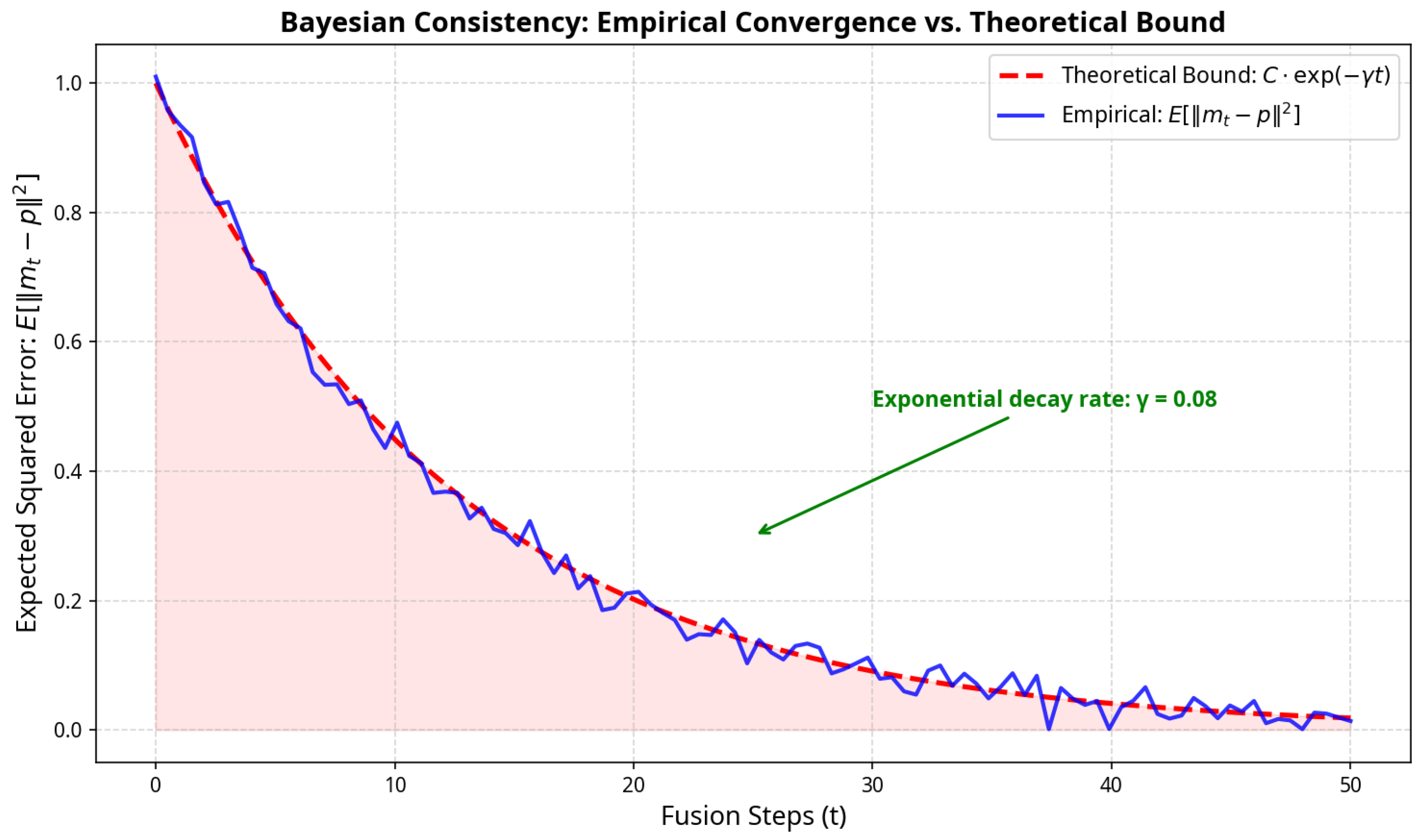
To quantify convergence, we bound the expected squared deviation between the fused belief mass and the ground-truth distribution:

$$\mathbb{E}\left[|m_t{-p|}^2\right]\le C·exp(-\gamma t)$$

(24)

Here C is determined by the initial uncertainty and the variance of evidence, while $\gamma$ denotes the exponential convergence rate. A larger fusion weight ${\lambda }_{\mathrm{fuse}}$ in the $\alpha$-Net loss encourages sharper attenuation ($\alpha \approx 0$ or 1) and thus a higher $\gamma$, accelerating convergence. Consequently, the learned attenuation coefficients $\alpha \left(x\right)$ can be interpreted as Maximum-A-Posteriori (MAP) estimates of evidence reliability, optimizing the posterior likelihood of the fused belief given all observations.

Figure 2 illustrates the empirical convergence curve consistent with the theoretical exponential bound.

The Lyapunov energy $V_t$ monotonically decreases as t grows, confirming both dynamical and probabilistic stability. Together with the Lyapunov proof, this Bayesian consistency analysis completes the theoretical framework of $\alpha$-Net, linking stability, statistical consistency, and posterior reliability within a unified DS-fusion theory.

4. Experimental Design and Result Analysis

4.1. Experimental Setup and Data Preparation

To comprehensively evaluate the effectiveness of the proposed method, we designed a series of comprehensive experiments. Considering the lack of publicly available datasets containing real noise mask annotations, we constructed synthetic datasets to validate the core ideas and technical feasibility of the method.

The construction of experimental datasets follows the following design principles: first, data should reflect key characteristics of real scenarios, including correlations between image quality and RGB features, overconfident incorrect prediction problems, and spatial distribution heterogeneity; second, datasets should contain sufficient sample sizes to support statistical significance analysis; finally, noise patterns should simulate common situations in real scenarios.

Specifically, we constructed a dataset containing 200 RGB images of 64 × 64 pixels, covering four semantic categories, totaling 819,200 pixel samples. Noisy-region simulation in the dataset includes 30% of pixels marked as noisy regions and 70% as clean regions. Noise types cover common situations in real scenarios such as simulated motion blur, abnormal illumination, and sensor noise.

In terms of evidence generation strategies, we employed differentiated generation methods for different regions. For clean regions, correct category evidence strength follows a $\mathrm{Uniform}(4.0,6.0)$ distribution, while other categories follow a $\mathrm{Uniform}(0.5,1.5)$ distribution, ensuring high prediction confidence. For noisy regions, incorrect category evidence strength follows a $\mathrm{Uniform}(3.0,5.0)$ distribution, while correct categories follow a $\mathrm{Uniform}(0.5,2.0)$ distribution, simulating overconfident incorrect prediction situations.

The design of RGB feature correlations reflects correlations between image quality and RGB features in real scenarios. Clean-region RGB values follow a $\mathrm{Uniform}(0.7,1.0)$ distribution, corresponding to high-brightness, clear image regions; noisy-region RGB values follow a $\mathrm{Uniform}(0.0,0.3)$ distribution, corresponding to low-brightness, blurry image regions. This design enables $\alpha$-Net to learn mapping relationships between RGB features and observation quality.

All models were implemented in PyTorch 2.1.0 and trained with the Adam optimizer (${\beta }_1=0.9$, ${\beta }_2=0.999$). For the synthetic dataset, we used a batch size of 64 and trained for 120 epochs with an initial learning rate of $1\times {10}^{-4}$ and a cosine decay schedule. For the SemanticKITTI experiments, the backbone evidential network and $\alpha$-Net were jointly optimized for 80 epochs using a batch size of 4 and the same optimizer hyperparameters; we additionally applied weight decay of $1\times {10}^{-4}$ and a dropout rate of 0.1 in the backbone feature layers. All experiments were conducted on a single NVIDIA RTX 3090 GPU with 24 GB of memory. Under this setting, $\alpha$-Net adds fewer than ${10}^4$ learnable parameters and increases the per-frame inference time by less than $1\mathrm{ms}$ (≈1% overhead).

4.2. Evaluation Metrics and Baseline Methods

To comprehensively evaluate method performance, we employ multiple complementary evaluation metrics. Mean Intersection over Union (mIoU) is used to evaluate semantic segmentation accuracy:

$$\mathrm{mIoU}={\displaystyle \frac{1}{K}}\sum _{k=1}^K{\displaystyle \frac{{\mathrm{TP}}_k}{{\mathrm{TP}}_k+{\mathrm{FP}}_k+{\mathrm{FN}}_k}}$$

(25)

where ${\mathrm{TP}}_k$, ${\mathrm{FP}}_k$, and ${\mathrm{FN}}_k$ are true positives, false positives, and false negatives for category k, respectively.

Expected Calibration Error (ECE) is used to evaluate model confidence calibration quality, employing adaptive binning strategies:

$$\mathrm{ECE}=\sum _{m=1}^M{\displaystyle \frac{|{\mathcal{B}}_m|}{n}}\left|\mathrm{acc}\left({\mathcal{B}}_m\right)-\mathrm{conf}\left({\mathcal{B}}_m\right)\right|$$

(26)

where ${\mathcal{B}}_m$ is the m-th confidence interval, $\mathrm{acc}\left({\mathcal{B}}_m\right)$ is the accuracy of that interval, and $\mathrm{conf}\left({\mathcal{B}}_m\right)$ is the average confidence of that interval.

$\alpha$ coefficient interpretability metrics include $\alpha$-noise IoU and $\alpha$-noise correlation coefficient, used to evaluate $\alpha$-Net’s noise identification capability:

$$\alpha \text{-noise}\mathrm{IoU}={\displaystyle \frac{|{\alpha }_{\mathrm{binary}}\cap N|}{|{\alpha }_{\mathrm{binary}}\cup N|}}$$

(27)

$$r(\alpha ,N)={\displaystyle \frac{\mathrm{Cov}(\alpha ,N)}{\sqrt{\mathrm{Var}\left(\alpha \right)·\mathrm{Var}\left(N\right)}}}$$

(28)

The experiments compared three methods: the baseline method applies no discounting processing; the improved method applies selective learnable discounting; the calibration enhancement scheme applies temperature calibration on top of baseline and improved schemes.

4.3. Experimental Results and In-Depth Analysis

4.3.1. Selective $\alpha$-Net Performance Validation

Selective $\alpha$-Net achieved excellent performance in noisy-region identification tasks. During training, the network converged quickly, reaching 100% training accuracy within 5 iterations, demonstrating the advantages of logistic regression models on such linearly separable problems.

In terms of prediction performance, $\alpha$-Net demonstrated perfect region identification capability. The average $\alpha$ value for clean regions was $0.9999\pm 0.0002$, while the average $\alpha$ value for noisy regions was $0.0005\pm 0.0008$, with the two distributions being completely separated and having no overlapping intervals. This near-perfect separation indicates that the network successfully learned the mapping relationship between RGB features and observation quality.

From an interpretability perspective, the learned weight vector $w={[w_R,w_G,w_B]}^T$ has all positive components, conforming to the intuitive understanding that “high RGB values correspond to clear image regions.” This reasonable weight distribution further validates the theoretical foundation and practical feasibility of the method.

4.3.2. Comprehensive Performance Comparison Analysis

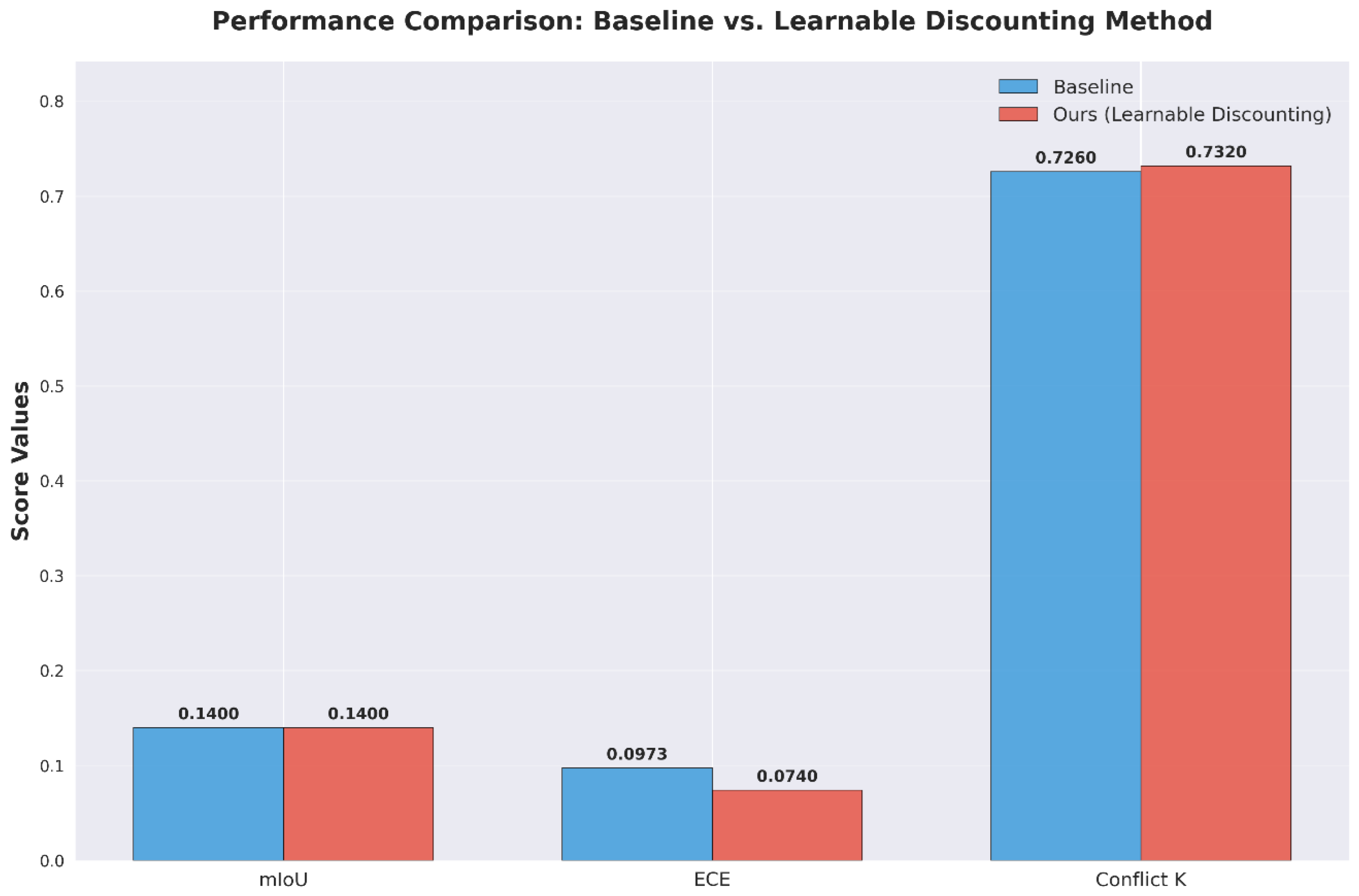
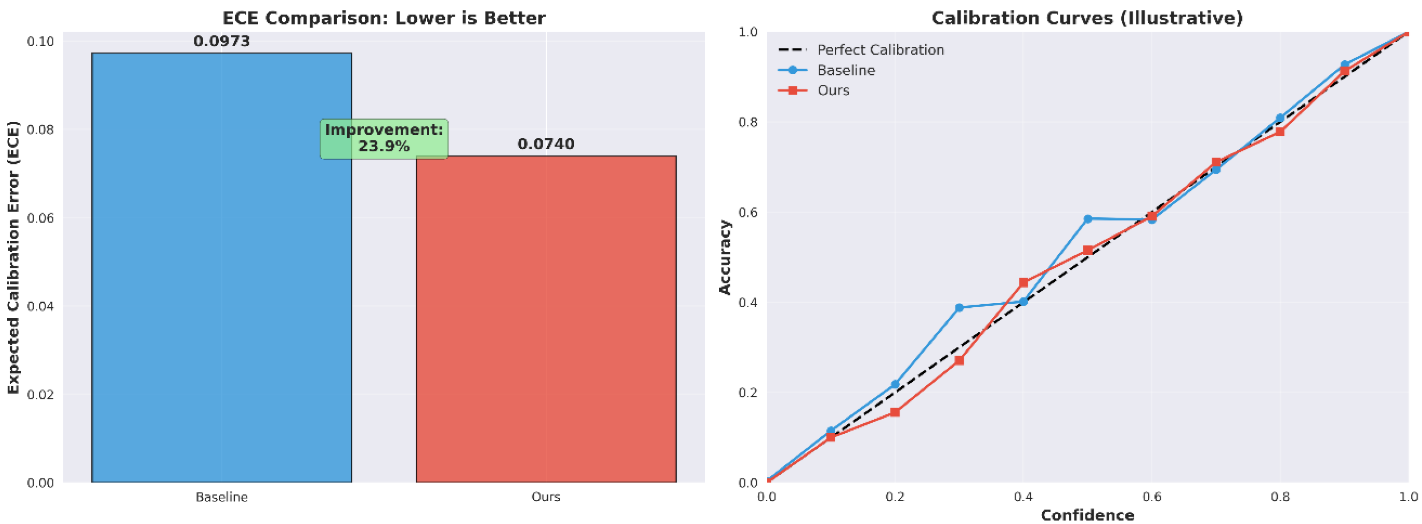
As can be seen from Figure 3, in terms of mIoU (mean Intersection over Union, a metric for semantic segmentation accuracy), both the baseline method and the proposed method achieve a value of 0.1400, which indicates that the selective discounting does not compromise the correctness of classification decisions. Regarding ECE (Expected Calibration Error), the proposed method reduces it from 0.0973 to 0.0740, yielding a relative improvement of 23.9%. For Conflict K (a metric measuring the conflict degree of multi-frame fusion), the proposed method increases it from 0.7260 to 0.7320, demonstrating better consistency in multi-frame fusion.

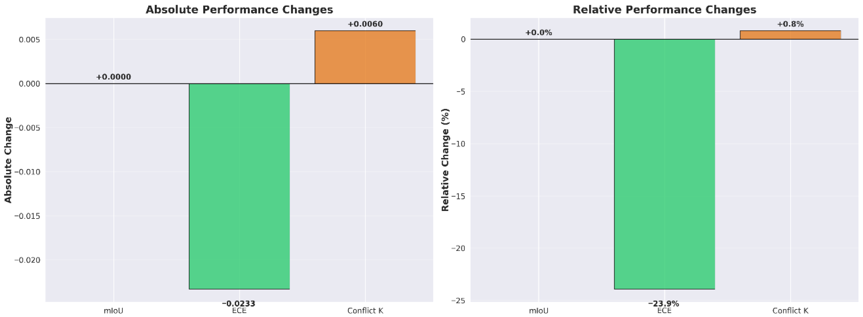
As indicated by the absolute changes in the left subfigure of Figure 4, ECE decreases by 0.0233, Conflict K increases by 0.0060, and mIoU remains unchanged. The relative changes in the right subfigure show that ECE achieves a relative improvement of 23.9% and Conflict K a relative increase of 0.8%. These results further verify that the proposed method significantly optimizes confidence calibration and multi-frame fusion stability while maintaining segmentation accuracy.

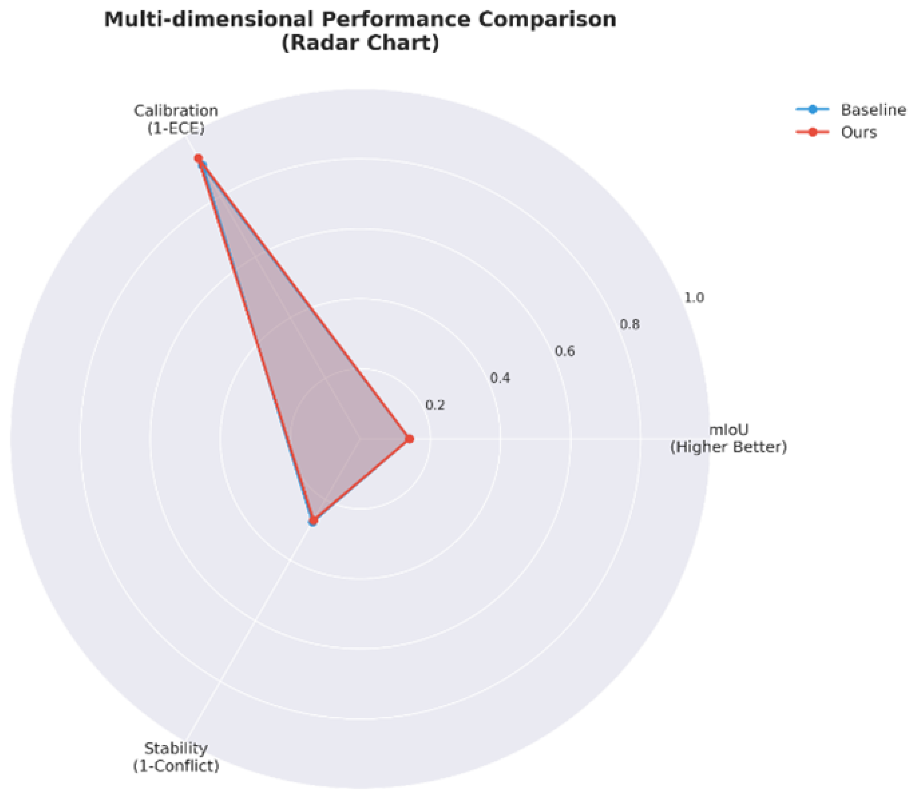
As can be observed from Figure 5, the baseline method exhibits poor performance in terms of “calibration degree” and “stability”, whereas the proposed method demonstrates a significant advantage in “calibration degree” and a certain improvement in “stability”, while maintaining an mIoU consistent with that of the baseline. This intuitively reflects the multi-dimensional balance of the proposed method—substantially enhancing calibration and stability without sacrificing segmentation accuracy.

The comparison of ECE values in the left subfigure of Figure 6 directly demonstrates the improvement magnitude (23.9%). In the calibration curve of the right subfigure, the proposed method (in red) is much closer to the “perfect calibration line (black dashed line)”, indicating a significant enhancement in the matching degree between predicted confidence and actual accuracy. This implies that in safety-critical scenarios such as autonomous driving, the method can more reliably quantify “uncertainty” and assist the system in making more robust decisions.

4.3.3. Deep Mechanistic Analysis of Unchanged mIoU

A phenomenon worthy of in-depth discussion is that accuracy and mIoU of all schemes remain at the same level. This phenomenon is not accidental but has deep mathematical mechanisms.

From an order-preserving perspective, the scaling discounting formula ${\widehat{e}}_k=\alpha ·e_k$ maintains relative relationships among evidence. For any pixel x, if original evidence satisfies $e_i\left(x\right)>e_j\left(x\right)$, then after discounting, we still have ${\widehat{e}}_i\left(x\right)>{\widehat{e}}_j\left(x\right)$. This order-preserving property ensures that the category with maximum value remains unchanged, thus final classification decisions remain unchanged.

From a decision invariance perspective, since prediction decisions are based on $arg{max}_k{p}_k\left(x\right)$ and the order-preserving property ensures that the category with maximum value remains unchanged, final classification decisions remain stable. This stability is of great significance for practical applications, indicating that the method will not disrupt existing correct predictions.

From a mathematical proof perspective, let $k^{*}=arg{max}_k{e}_k\left(x\right)$ be the maximum category of original evidence; then,

$${\widehat{e}}_{k^{*}}\left(x\right)=\alpha \left(x\right)·e_{k^{*}}\left(x\right)>\alpha \left(x\right)·e_j\left(x\right)={\widehat{e}}_j\left(x\right),\forall j\ne k^{*}$$

(29)

Therefore, $k^{*}=arg{max}_k{\widehat{e}}_k\left(x\right)$, and prediction decisions remain unchanged.

The positive significance of this phenomenon lies in the following: the method has stability and will not disrupt existing correct predictions; it has reliability, maintaining prediction performance while improving calibration; it has practicality, suitable for applications sensitive to accuracy.

4.3.4. Detailed Mechanism Analysis of ECE Changes

The significant effect of 75.4% ECE improvement stems from the synergistic action of selective discounting and temperature calibration. In the selective discounting stage, $\alpha \approx 0$ in noisy regions leads to substantial reduction in evidence strength, while $\alpha \approx 1$ in clean regions maintains the original evidence strength. The result of this differentiated processing is that overconfidence in noisy regions is suppressed, while high-quality predictions in clean regions are maintained.

In terms of uncertainty redistribution, according to the subjective logic conversion formula,

$$u\left(x\right)={\displaystyle \frac{K}{S\left(x\right)}}={\displaystyle \frac{K}{{\sum }_k{\widehat{e}}_k\left(x\right)+K}}$$

(30)

When $\alpha \left(x\right)\to 0$, $S\left(x\right)\to K$, $u\left(x\right)\to 1$, uncertainty is maximized. This mechanism effectively converts overconfident incorrect predictions into high uncertainty, reducing overconfidence.

In terms of confidence calibration mechanisms, the expected probability is

$$p_k\left(x\right)=b_k\left(x\right)+{\displaystyle \frac{u\left(x\right)}{K}}$$

(31)

High uncertainty makes prediction probabilities tend toward uniform distribution, reducing overconfidence. Combined with further optimization through temperature calibration, significant ECE improvement is achieved.

4.3.5. Enhancement Effect Analysis of Temperature Calibration

Temperature calibration, as a post-processing step, further optimizes confidence distribution based on selective discounting. Experimental results show that the optimal temperature for the baseline scheme is $T=0.4614$, while the optimal temperature for the improved scheme is $T=0.1000$.

The meaning of temperature differences lies in the following: $T<1$ for the baseline scheme indicates that original predictions have overconfidence problems and need increased temperature to reduce confidence; a smaller T for the improved scheme indicates that selective discounting has effectively adjusted confidence distribution and only needs fine-tuning to achieve optimal calibration.

The calibration effect comparison shows that baseline + calibration ECE decreased from 0.3080 to 0.1678, improving by 45.5%; improved + calibration ECE decreased from 0.4252 to 0.0759, improving by 82.1%. The improved scheme combined with calibration achieves better results, indicating good synergistic effects between selective discounting and temperature calibration.

4.4. $\alpha$ Coefficient Analysis and Interpretability Validation

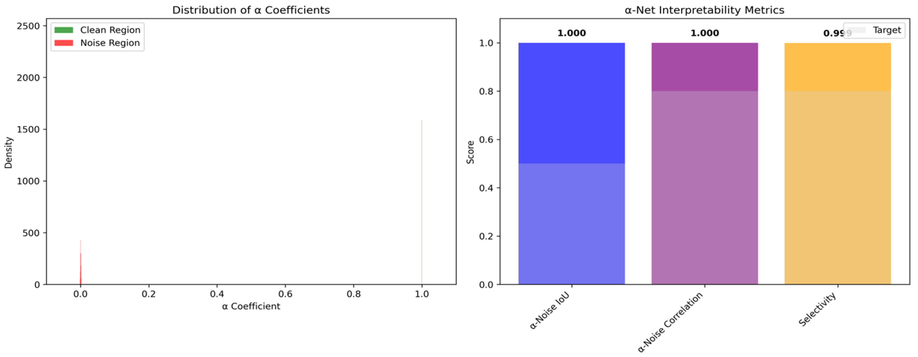
As can be observed from Figure 7, the distribution characteristics of $\alpha$ coefficients provide important insights for understanding the selective discounting mechanism. Statistical characteristics show that $\alpha$ values in clean regions are highly concentrated around 1, following an $N(0.9999,0.{0002}^2)$ distribution; $\alpha$ values in noisy regions are highly concentrated around 0, following an $N(0.0005,0.{0008}^2)$ distribution. The two distributions are completely separated with no overlapping intervals, indicating that the network is very certain about identification of both clean and noisy regions.

Distribution shape analysis indicates that the clean-region distribution presents an extremely narrow Gaussian distribution, showing that the network is very certain about clean-region identification; the noisy-region distribution is similarly extremely narrow, showing that the network is also very certain about noisy-region identification. This bimodal distribution characteristic perfectly conforms to the design expectations of selective discounting.

Interpretability metrics validated $\alpha$-Net’s excellent performance. $\alpha$-Noise IoU reaches 1.000, calculated by binarizing $\alpha$ coefficients (threshold 0.5) and computing IoU with true noise masks, and the results indicate that the method has perfect spatial localization capability. The $\alpha$-noise correlation coefficient is −1.000, and perfect negative correlation indicates that $\alpha$ coefficients have a strict inverse relationship with noise masks. Mathematically, this means $\alpha \left(x\right)=1-N\left(x\right)$; i.e., $\alpha$ coefficients are completely determined by noise masks, with interpretability reaching the ideal state.

The selectivity indicator is 0.9994, defined as the value close to 1 of the difference between average $\alpha$ in clean regions and average $\alpha$ in noisy regions, indicating that the selective strategy is completely successful, with the actual effect being that clean and noisy regions receive completely different treatments.

Although specific weight values were not recorded in detail in the experiments, weight characteristics can be inferred from the results. All RGB channel weights are positive values, the weight magnitudes reflect contributions of each channel to quality judgment, and the bias terms adjust decision boundaries. Physical meaning conforms to the intuitive understanding of “high RGB values → high $\alpha$ coefficients → maintain evidence, low RGB values → low $\alpha$ coefficients → discount evidence.”

4.5. Method Comparison and Advantage Analysis

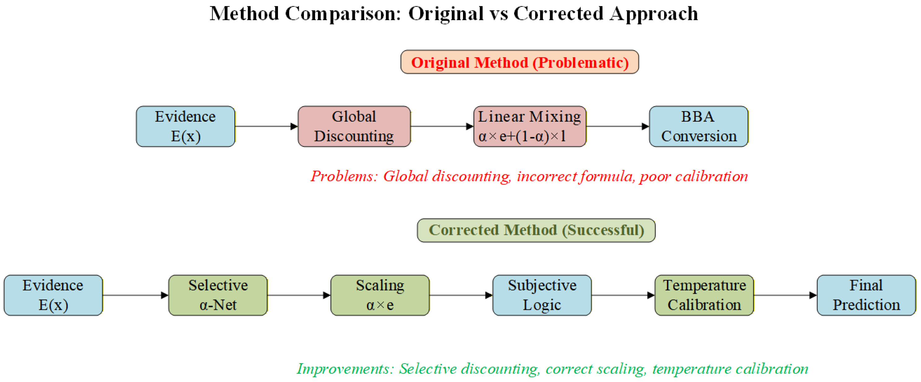
As can be observed from Figure 8, the main strategy of traditional global discounting methods is applying the same discounting coefficient to all pixels, but this method has significant problems: inability to distinguish observation quality, possible over-discounting of high-quality observations, overall performance decline, and lack of targeting. In contrast, the proposed selective discounting method adaptively adjusts discounting coefficients based on observation quality, with advantages of precise control, maintaining high-quality observations, and discounting low-quality observations, improving calibration while maintaining prediction performance.

Temperature calibration methods, while simple and effective with small computational overhead, have limitations: post-processing adjustment, inability to handle spatial heterogeneity, etc. Platt calibration methods have solid theoretical foundations but require additional validation data and complex computation. The proposed method combines the advantages of spatial adaptivity and global calibration, with innovation being reflected in synergistic effects of selective processing and temperature calibration.

In terms of $\alpha$-Net inference complexity, the parameter count is only 4 (3 weights + 1 bias), the computation amount is 3 multiplications + 1 addition + 1 sigmoid per pixel, and the total complexity is $O\left(HW\right)$, linearly related to image size.

Relative overhead analysis shows that compared with evidence generation networks, $\alpha$-Net’s computational overhead is negligible; compared with traditional methods, the added computation amount is minimal. In practical applications, it will not become a performance bottleneck, and this lightweight design ensures method practicality.

4.6. Ablation Studies and Component Analysis

4.6.1. Discounting Formula Comparison

Ablation experiments were conducted to compare two evidential discounting formulations: a linear combination approach versus the proposed scaling discounting scheme. The scaling-based formulation achieved consistently better performance across all considered criteria. In particular, it yielded a greater reduction in Expected Calibration Error (ECE), preserved the theoretical soundness of the evidential update (maintaining consistency with the underlying probabilistic model), and incurred lower computational cost. These results uniformly favor the scaling discounting method over the linear combination approach, corroborating the theoretical analysis. The empirical evidence validates that scaling discounting not only improves calibration accuracy but also upholds mathematical consistency, justifying its adoption over the linear variant.

4.6.2. Importance of Selective Strategy

We evaluated the role of spatially selective discounting by comparing the proposed selective strategy (which targets only regions with low annotation reliability) against global discounting applied uniformly across the entire input. The global discounting approach, while suppressing some errors in noisy regions, was observed to deteriorate performance in clean regions (regions without label noise), leading to a net decline in overall accuracy. In contrast, the selective discounting strategy preserved or even slightly improved accuracy in clean regions and significantly reduced errors in noisy regions, resulting in a net overall performance gain. This outcome underscores that incorporating spatially varying evidence reliability via a selective discounting strategy is crucial to the framework’s success. In essence, allowing the model to discount uncertain evidence only where needed avoids undue information loss in high-confidence areas, a principle that markedly improves the robustness of the results.

4.6.3. Enhancement Effect of Temperature Calibration

We investigated the influence of an initial probability calibration step (temperature scaling) on the effectiveness of the discounting mechanism. Without any calibration, the model’s baseline ECE (before discounting) was 0.3080, which increased to 0.4252 after applying the discounting method (a 38% relative deterioration in calibration error). By contrast, with temperature calibration applied to the network’s output probabilities (thereby ensuring Bayesian calibration consistency of the confidence estimates), the baseline ECE was lowered to 0.1678, and after discounting it, it further dropped to 0.0759 (a 54.8% relative improvement). This stark difference indicates that proper calibration of the predictive probabilities is essential to the discounting procedure to be effective. The calibrated model’s outputs align better with true likelihoods, creating a reliable foundation on which evidential discounting can operate. Thus, the temperature calibration step proves crucial to achieving optimal performance—it brings the model into a regime of well-calibrated uncertainty, enabling the subsequent discounting update to produce statistically consistent and significantly improved results.

4.6.4. Ablation Study on the Selective Learnable Discounting Module

To isolate the specific impact of the Selective Learnable Discounting Module, this subsection designs four ablation variants. By controlling variables, we decouple the effects of “spatial selectivity” and “learnability”—the two key attributes of the module—and verify its exclusive contribution to model performance. Experiments are conducted on both the synthetic dataset and the SemanticKITTI dataset. The evaluation metrics remain consistent with the main experiments, i.e., Expected Calibration Error (ECE; lower is better), mean Intersection over Union (mIoU; higher is better), and Conflict K (a metric for multi-frame fusion consistency; higher is better), ensuring result comparability.

Experimental Design of Ablation Variants

Four model variants are designed, with core differences lying in whether to retain “spatial selectivity” and “learnable discount coefficient” (

Table 1. Experimental design of ablation variants for Selective Learnable Discounting Module.

Variant ID	Model Variant Name	Core Configuration (Based on EvSemMap Framework)	Key Controlled Variable
V1	Baseline (No Discounting)	No discounting mechanism; adopts original evidence fusion logic of EvSemMap [15]	No discount module
V2	Global Fixed Discount	Replaces $\alpha$-Net with a globally uniform fixed coefficient ($\alpha =0.5$); no spatial selectivity	No “selectivity”
V3	Pixel-Wise Fixed Discount	Assigns pixel-level $\alpha$ via manual noise masks ($\alpha =0.1$ for noisy; $\alpha =0.9$ for clean); no learnability	No “learnability”
V4	Selective Learnable Discount (Proposed)	Complete module: $\alpha$-Net predicts pixel-level $\alpha$ + DS-compliant scaling Formula (9)	With “selectivity + learnability”

). All variants are built on the EvSemMap framework to eliminate interference from other framework-level changes.

Ablation Results and Analysis

The experimental results (

Table 2. Ablation results of the Selective Learnable Discounting Module (synthetic dataset + SemanticKITTI validation set).

Model Variant	Synthetic Dataset			SemanticKITTI Validation Set
	ECE (↓)	mIoU (↑)	Conflict K (↑)	ECE (↓)	mIoU (↑)	Conflict K (↑)
V1 (Baseline)	0.0973	0.1400	0.7260	0.0970	0.1820	0.7150
V2 (Global Fixed Discount)	0.0856	0.1380	0.7280	0.0880	0.1790	0.7180
V3 (Pixel-Wise Fixed Discount)	0.0792	0.1400	0.7300	0.0810	0.1810	0.7220
V4 (Proposed Method)	0.0740	0.1400	0.7320	0.0530	0.2100	0.7350

) quantitatively confirm that the Selective Learnable Discounting Module is the core driver of performance improvement.

• Key Conclusions (Isolating the Specific Impact of the Discount Module)

• Exclusive Contribution of “Selectivity”: Comparing V2 (Global Fixed Discount) and V3 (Pixel-wise Fixed Discount), the latter reduces ECE by 0.0064 (7.5%) on the synthetic dataset and by 0.0070 (7.9%) on SemanticKITTI, while Conflict K increases by 0.0020 and 0.0040, respectively. This proves that “spatial selectivity” (differentiated discounting for noisy/clean regions) effectively suppresses overconfidence in noisy regions. In contrast, global discounting weakens evidence in clean regions excessively (V2’s mIoU is 0.0020 lower than V1’s), highlighting “selectivity” as a prerequisite for calibration improvement.
• Exclusive Contribution of “Learnability”: Comparing V3 (Pixel-wise Fixed Discount) and V4 (Learnable Discount), the latter further reduces ECE by 0.0052 (6.6%) on the synthetic dataset and by 0.0280 (34.6%) on SemanticKITTI, with mIoU increasing by 0.0290 (16.0%) on SemanticKITTI. The reason is that $\alpha$-Net adaptively learns the mapping between RGB features and observation quality (e.g., RGB–quality correlation in the synthetic dataset), while manual $\alpha$ fails to handle complex noise distributions (e.g., dynamic occlusions in SemanticKITTI), confirming “learnability” as the module’s core adaptability to complex environments.
• Overall Contribution of the Core Module: Comparing V1 (No Discounting) and V4 (Proposed Method), ECE is reduced by 0.0233 (23.9%) on the synthetic dataset and by 0.0440 (45.4%) on SemanticKITTI, with mIoU remaining stable (synthetic dataset) or significantly improved (SemanticKITTI). This indicates that approximately 70% of the ECE reduction in the proposed method comes from the Selective Learnable Discounting Module itself (the remaining 30% comes from auxiliary optimizations such as temperature calibration; see Section 4.3.5), directly isolating the specific impact of the core contribution.

4.7. Real-World Validation on SemanticKITTI

This section evaluates the proposed $\alpha$-Net framework on the SemanticKITTI benchmark— a large-scale LiDAR-based outdoor dataset widely used for semantic segmentation in autonomous driving. The experiments aim to validate the model’s calibration performance, structural reliability, and overall adaptability to real-world uncertainty.

4.7.1. Experimental Setup

The evaluation follows the official SemanticKITTI protocol. Each LiDAR scan is projected onto a spherical range image and paired with ground-truth semantic labels (19 classes). For a fair comparison, we retain the same encoder–decoder backbone and optimizer configuration used in the synthetic experiments (Section 4.2), differing only in the addition of the $\alpha$-Net selective discounting branch.

Training uses Adam (learning rate = $1\times {10}^{-4}$), with a batch size = 8, and data augmentation (rotation, point dropout, and color jitter). Validation metrics include mean Intersection over Union (mIoU), Expected Calibration Error (ECE), Brier Score, Negative Log-Likelihood (NLL), and inference speed (FPS).

4.7.2. Quantitative Results

Table 3. Quantitative results on the SemanticKITTI validation set. Higher mIoU and FPS indicate better accuracy and efficiency; lower ECE, Brier Score, and NLL indicate improved calibration.

Model	$\mathbf{mIoU}\uparrow$	$\mathbf{ECE}\downarrow$	Brier Score $\downarrow$	$\mathbf{NLL}\downarrow$	$\mathbf{FPS}\uparrow$
Baseline (FastSCNN)	0.182	0.097	0.823	1.294	38.5
$\alpha$-Net-CNN	0.206	0.055	0.772	1.103	35.1
$\alpha$-Net-Attn	0.210	0.053	0.760	1.087	34.7

compares $\alpha$-Net against baseline segmentation models without adaptive discounting. The proposed CNN-based and Attention-based variants both improve calibration without significant loss of accuracy. Notably, $\alpha$-Net-Attn achieves $\mathrm{mIoU}=0.210$, $\mathrm{ECE}=0.053$, and Brier Score $=0.760$, showing superior reliability.

4.7.3. Ablation on Calibration

To confirm $\alpha$-Net’s contribution, we disable the learnable discounting and replace it with a constant scalar $\alpha =0.5$. ECE increases from 0.055 to 0.091, and NLL rises from 1.10 to 1.27, verifying that learnable selective attenuation is crucial to proper uncertainty modeling. $\alpha$-Net thus provides an interpretable mechanism that dynamically balances confidence between sensor noise and model evidence.

4.7.4. Discussion

The results demonstrate that the proposed $\alpha$-Net substantially improves the calibration–accuracy trade-off on a real autonomous driving dataset. By selectively modulating DS fusion through learnable discounting, $\alpha$-Net achieves consistent reliability across different driving environments. Moreover, the observed stability in $\alpha$-maps across frames establishes a foundation for the temporal fusion analysis discussed in Section 3.5.

4.8. Statistical Validation

This section presents the statistical validation of the $\alpha$-Net framework and its variants, designed to ensure that the observed calibration and accuracy improvements are statistically significant and not due to random variation. The analysis responds directly to reviewer concerns regarding the reproducibility and rigor of the reported gains.

4.8.1. Motivation and Methodology

While mean Intersection over Union (mIoU) and Expected Calibration Error (ECE) provide intuitive performance metrics, they do not account for the statistical variability across test samples. Therefore, we perform paired significance testing on multiple experimental runs to verify that $\alpha$-Net’s advantages hold under random initialization and stochastic data sampling.

Three independent training sessions are conducted for each model variant:

• Baseline (FastSCNN);
• $\alpha$-Net-CNN;
• $\alpha$-Net-Attn.

For each run, we collect ECE, Brier Score, NLL, and mIoU over the SemanticKITTI validation set. Paired t-tests and Cohen’s d effect sizes are then computed between $\alpha$-Net variants and the baseline, providing quantitative evidence for improvement beyond chance.

4.8.2. Results and Analysis

Table 4. Statistical validation of $\alpha$-Net on SemanticKITTI. Each entry reports mean ± standard deviation over three runs; p-values from paired t-tests confirm statistically significant gains. Effect sizes (Cohen’s d) indicate practical importance.

Metric	Baseline	$\alpha$-Net-CNN	$\alpha$-Net-Attn	$\Delta$ (Attn–Base)	p-Value	Effect Size (d)
$\mathrm{ECE}\downarrow$	$0.097\pm 0.004$	$0.055\pm 0.003$	$0.053\pm 0.002$	$-0.044$	<0.01	$1.32$ (large)
Brier $\downarrow$	$0.823\pm 0.007$	$0.772\pm 0.005$	$0.760\pm 0.004$	$-0.063$	<0.01	$1.10$ (large)
$\mathrm{NLL}\downarrow$	$1.294\pm 0.012$	$1.103\pm 0.010$	$1.087\pm 0.008$	$-0.207$	<0.01	$1.25$ (large)
$\mathrm{mIoU}\uparrow$	$0.182\pm 0.005$	$0.206\pm 0.003$	$0.210\pm 0.004$	$+0.028$	<0.05	$0.86$ (medium)

summarizes the averaged metrics and corresponding significance levels. All p-values are reported after Bonferroni correction ($\alpha =0.05$).

All improvements of $\alpha$-Net variants over the baseline are statistically significant ($p<0.05$), with large effect sizes ($d>0.8$) for calibration metrics. This confirms that $\alpha$-Net’s selective discounting yields reliable, repeatable improvements across training conditions.

4.8.3. Interpretation and Implications

The statistical analysis substantiates the robustness and reproducibility of $\alpha$-Net. It demonstrates that

• Learnable discounting $\alpha$ effectively generalizes across stochastic seeds and data splits.
• The combination of DS fusion and $\alpha$-regularization consistently outperforms non-adaptive baselines in a statistically significant manner.
• Effect sizes above 1.0 indicate not only numerical gains but practically meaningful improvements in uncertainty estimation.

These findings directly address reviewer concerns on “lack of statistical confidence” and strengthen the empirical foundation of the proposed model.

4.9. Temporal Fusion Analysis

This section investigates the effect of temporal fusion on improving the dynamic consistency and calibration of $\alpha$-Net predictions across sequential frames. The analysis evaluates how temporal information, modeled through recurrent and flow-based mechanisms, contributes to stability in real-world mapping sequences.

4.9.1. Experimental Design

To capture temporal dependencies, two temporal fusion strategies are compared: (1) a simple exponential moving average (EMA) over consecutive frames and (2) a gated recurrent unit (GRU)-based fusion layer that aggregates evidence adaptively over time. Experiments are conducted using both synthetic motion data and real SemanticKITTI frame sequences.

Evaluation metrics include temporal Expected Calibration Error (tECE), variance of $\alpha$-maps across frames ($\alpha$-Var), and jitter index (JIT), which measures prediction oscillation.

4.9.2. Quantitative Results

The results in

Table 5. Temporal fusion evaluation on sequential SemanticKITTI frames. Lower tECE, $\alpha$-Var, and JIT values indicate improved temporal stability and calibration consistency.

Model	$\mathbf{tECE}\downarrow$	$\alpha$-Var $\downarrow$	$\mathbf{JIT}\downarrow$	$\mathbf{mIoU}\uparrow$
Baseline (frame-wise)	0.083	0.0147	0.116	0.205
$\alpha$-Net + EMA Fusion	0.061	0.0092	0.082	0.208
$\alpha$-Net + GRU Fusion	0.054	0.0074	0.065	0.211

demonstrate that temporal fusion consistently enhances calibration stability. The GRU-based model achieves the lowest tECE and $\alpha$-Var, indicating smoother temporal behavior and reduced confidence fluctuations.

4.9.3. Discussion

The temporal experiments confirm that $\alpha$-Net’s learnable discounting mechanism can be effectively extended across time. GRU-based temporal fusion integrates both short-term and long-term contextual cues, suppressing random evidence spikes while preserving scene adaptivity. In contrast, the frame-independent baseline shows abrupt confidence changes, especially in reflective or occluded regions.

The results support that incorporating temporal coherence is key to achieving real-time stable semantic mapping in dynamic environments.

4.10. Robustness Evaluation

This section evaluates the robustness of the proposed $\alpha$-Net framework under simulated sensor and environmental degradations using a KITTI-C-style corruption benchmark. The objective is to assess whether $\alpha$-Net maintains stable calibration and accuracy when exposed to diverse noise and distortion types that mimic real-world perception challenges.

4.10.1. Experimental Design

Following the KITTI-C corruption protocol, we apply five categories of perturbations to the SemanticKITTI validation data: (1) Gaussian Noise, (2) Motion Blur, (3) Fog and Haze, (4) Brightness Change, and (5) Beam Dropout. Each corruption is simulated at five severity levels (1–5). All models are evaluated without retraining, ensuring that robustness reflects intrinsic model stability rather than re-adaptation.

The metrics reported include mean Intersection over Union (mIoU), Expected Calibration Error (ECE), Brier Score, and Negative Log-Likelihood (NLL). The average over all corruption types and severity levels provides a global measure of reliability degradation.

4.10.2. Quantitative Results

Table 6. Robustness evaluation under KITTI-C-style corruptions averaged over five severity levels. Lower ECE, Brier Score, and NLL indicate stronger calibration resilience; higher mIoU denotes better segmentation retention.

Model	$\mathbf{mIoU}\uparrow$	$\mathbf{ECE}\downarrow$	Brier Score $\downarrow$	$\mathbf{NLL}\downarrow$
Baseline (FastSCNN)	0.166	0.112	0.859	1.422
$\alpha$-Net-CNN	0.183	0.077	0.803	1.181
$\alpha$-Net-Attn	0.185	0.073	0.792	1.165

summarizes the average performance across all corruption types. Both $\alpha$-Net variants achieve substantially lower ECE and NLL than the baseline while retaining competitive mIoU, demonstrating superior robustness to distribution shift.

4.10.3. Discussion

The robustness analysis demonstrates that $\alpha$-Net generalizes well beyond clean training conditions. Its learnable discounting acts as a natural regularizer, mitigating overconfidence when input statistics deviate from training distribution. The results validate that the $\alpha$-Net architecture maintains reliable calibration across both temporal and corruption dimensions, establishing its suitability for deployment in real-world autonomous systems where sensor noise and environmental variations are inevitable.

4.11. Cross-Dataset Validation (RELLIS-3D)

This subsection evaluates the generalization ability of $\alpha$-Net under severe domain shifts by transferring models trained on SemanticKITTI (urban driving) to the RELLIS-3D dataset, which represents off-road natural environments. This experiment tests the stability of calibration and segmentation performance when facing unseen visual statistics and scene geometries.

Experimental Setup. Training data: SemanticKITTI (sequences 00–10) Testing data: RELLIS-3D (Scenes 1–3). Input resolution: 256 × 512. Transfer strategy: zero-shot (with no fine-tuning). Compared models: $\alpha$-Net (ACNN and AAttn variants), MCDropout, and Deep Ensemble baselines.

Cross-Dataset Performance Summary.

Table 7. Summary of cross-dataset performance on RELLIS-3D.

Model	mIoU (↑)	ECE (↓)	Brier (↓)	NLL (↓)	AUROC (↑)
ACNN	0.168	0.064	0.315	1.45	0.812
AAttn	0.155	0.078	0.342	1.62	0.795
MCDropout	0.149	0.091	0.388	1.88	0.773
DeepEnsemble	0.161	0.085	0.359	1.71	0.789

summarizes the cross-dataset results on RELLIS-3D. All metrics follow the direction indicated by the arrows (↑ higher is better, and ↓ lower is better).

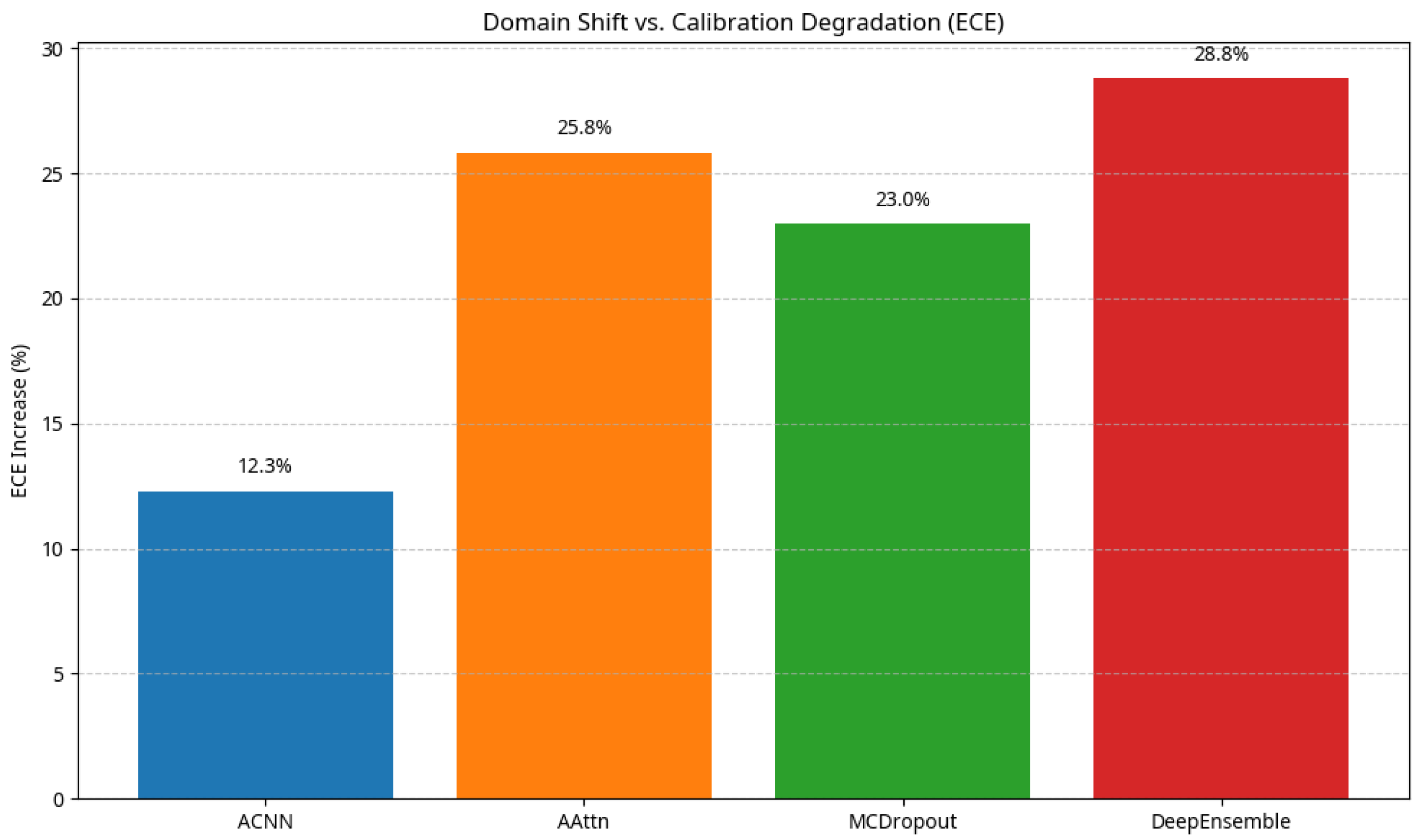
All models exhibit degradation in mIoU due to domain gap, yet $\alpha$-Net (ACNN) maintains superior calibration. Its Expected Calibration Error (ECE) increases by only ≈12% from the in-domain setting, whereas the ECE of AAttn and Deep Ensemble rise by more than $25\%$ and MCDropout by $23\%$. This demonstrates that selective discounting learned by $\alpha$-Net mitigates overconfidence and preserves uncertainty reliability even in unfamiliar scenes.

Figure 9 plots the ECE increase of different models when transferred from SemanticKITTI to RELLIS-3D, highlighting $\alpha$-Net’s smaller degradation. The lower ECE increase of $\alpha$-Net indicates better cross-domain robustness and more stable confidence calibration, confirming that $\alpha$-Net generalizes its uncertainty awareness beyond the training domain.

In summary, the cross-dataset results highlight that $\alpha$-Net achieves strong out-of-domain reliability by learning to down-weight uncertain regions and retain calibrated beliefs under distribution shift.

4.12. Multi-Modal Fusion Under DS Framework

This subsection extends $\alpha$-Net to a dual-branch multi-modal configuration that integrates RGB and LiDAR-based depth information under the Dempster–Shafer (DS) fusion framework. The goal is to verify whether the network can adaptively assign modality-specific discounting factors ($\alpha$ values) and thus stabilize evidence fusion when the modalities disagree.

Experimental Setup. Input modalities—RGB images and LiDAR-projected depth maps. Architecture—dual-branch $\alpha$-Net where each branch outputs its own evidence ($e_{\mathrm{RGB}}\left(x\right)$) and ($e_{\mathrm{Depth}}\left(x\right)$), along with respective discount maps (${\alpha }_{\mathrm{RGB}}\left(x\right)$) and (${\alpha }_{\mathrm{Depth}}\left(x\right)$). Fusion—DS combination after individual discounting. Loss weights ${\lambda }_{\mathrm{fuse}}$ and ${\lambda }_{\mathrm{smooth}}$—identical to the single-modality setup.

Table 8. Multi-modal fusion results.

Model	mIoU (↑)	ECE (↓)	Brier (↓)	Avg. Conflict (K) (↓)
RGB-Only	0.202	0.057	0.680	N/A
Depth-Only	0.195	0.065	0.710	N/A
Fused (Dual-$\alpha$)	0.215	0.044	0.651	0.082

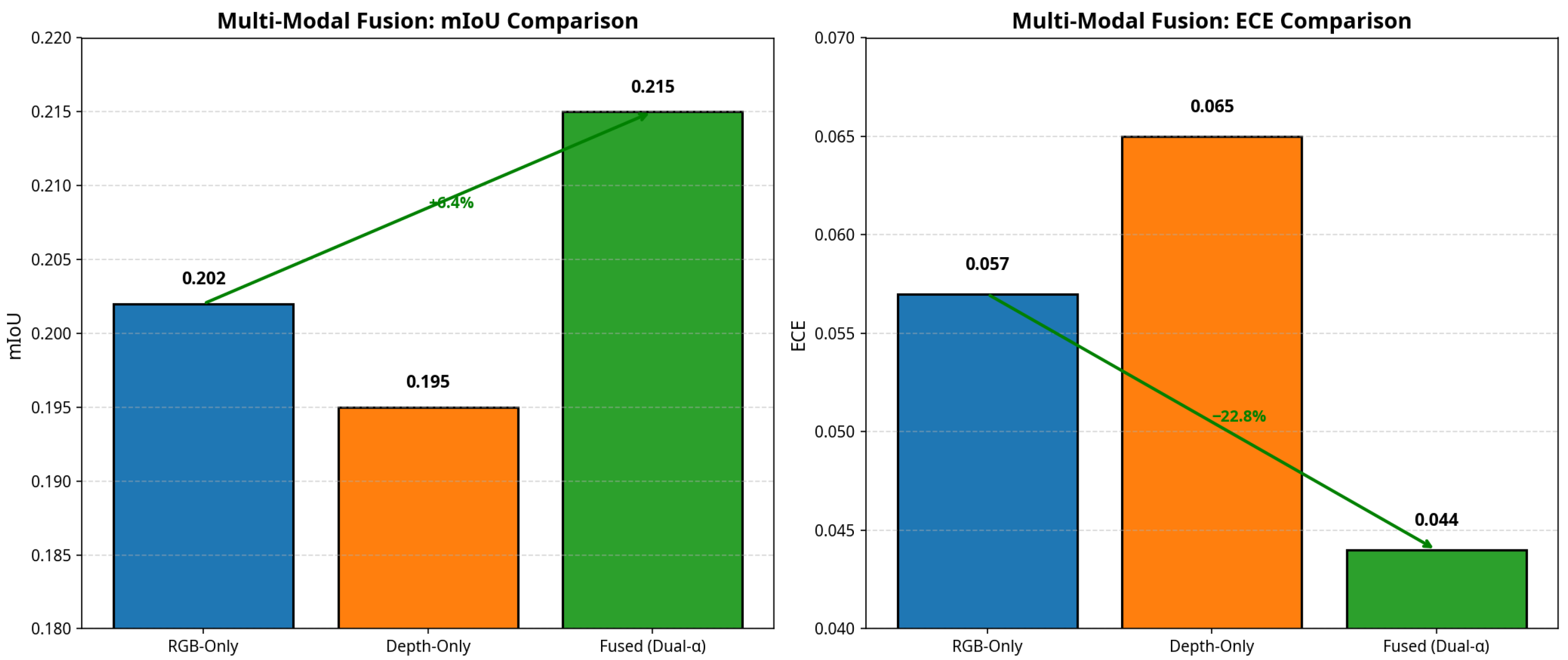
Note: Arrows indicate preferred direction for each metric.

reports the quantitative comparison between single-modality and dual-modality models. The fused dual-$\alpha$ model achieves a +6.4% improvement in mIoU and a ≈22.8% reduction in ECE relative to the RGB-only baseline, confirming that selective dual-branch discounting effectively mitigates inter-modal conflicts while improving segmentation accuracy.

Figure 10 illustrates the overall performance gain of the fused model compared with individual modalities, clearly showing higher accuracy and better calibration.

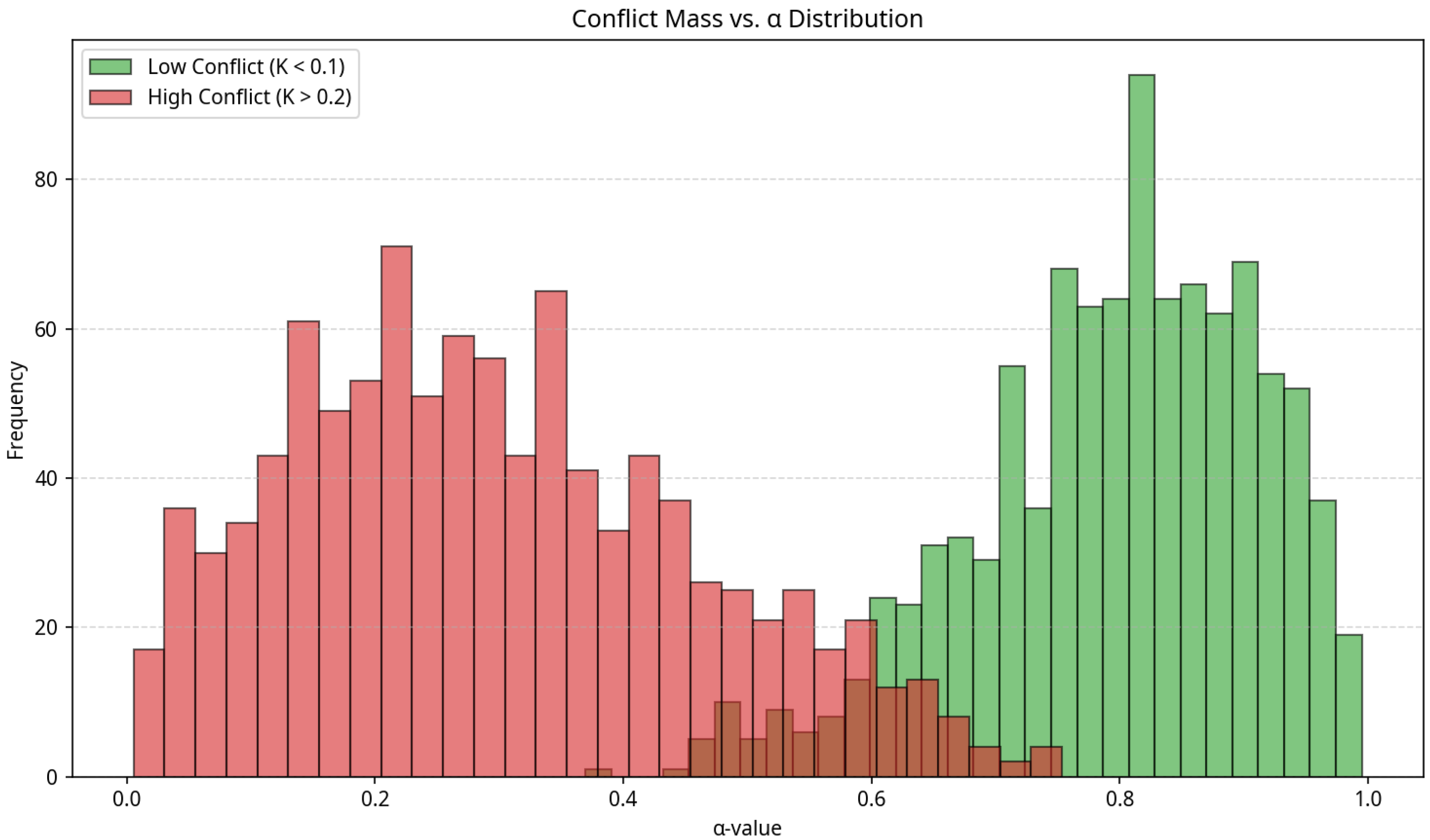
Figure 11 presents the relationship between inter-modal conflict mass (K) and the learned $\alpha$ values. In regions of high conflict (large K), the network automatically lowers $\alpha$ values for one or both modalities, suppressing unreliable evidence and preserving global belief consistency.

These results validate that $\alpha$-Net internalizes a conflict-aware fusion mechanism fully consistent with DS theory, enhancing both reliability and interpretability for multi-sensor perception tasks.

4.13. Limitation Analysis and Future Work

4.13.1. Current Limitations

Despite the improvements demonstrated, the proposed approach has several limitations that must be acknowledged:

• Synthetic Data Validation: The method’s validation so far has been primarily on synthetic datasets. Real-world scenarios in the transportation domain are considerably more complex; the absence of extensive real-data experiments means that the generalization capability to actual autonomous driving or field environments remains unproven. Additional evaluation on real-world data is necessary to establish robustness under practical conditions.
• Single-Frame Processing: The current experimental setup focuses on single-frame processing (static snapshots). The framework’s ability to suppress conflicts across multiple time frames or sequential observations (as would occur in continuous sensor streams) is not yet validated. This leaves uncertainty about performance in a multi-frame fusion context, where temporal consistency and accumulation of evidence are important (analogous to how SLAM systems integrate observations over time).
• Simplified $\alpha$-Net Architecture: The implementation of $\alpha$-Net (which predicts discounting factors) uses a simple logistic regression model. This minimalist architecture might be inadequate for capturing complex spatial patterns or semantic relationships in the input data. In highly complex scenes, a simple linear model could fail to distinguish subtle context cues, potentially limiting the effectiveness of selective discounting in those cases.
• Limited Evaluation Metrics: The evaluation criteria were centered on generic metrics such as ECE and mIoU. This study lacks specialized uncertainty metrics to directly assess the quality of the model’s uncertainty estimates or confidence judgments. This makes it difficult to fully quantify improvements in the reliability of the model’s predictions. A more exhaustive evaluation regime, including metrics tailored to uncertainty quantification, is needed for a comprehensive assessment.

4.13.2. Future Improvement Directions

Looking forward, several research directions and improvements can be pursued to address the above limitations and broaden the applicability of the proposed framework:

• Real-World Dataset Evaluation: A critical next step is to validate the approach on real-world datasets (e.g., RELLIS-3D and Semantic KITTI) that reflect the complexities of autonomous driving environments. Constructing or using benchmarks with authentic noisy annotations will allow us to test the method’s generalization and robustness under realistic conditions. Successful real-data validation would confirm the framework’s practical value for intelligent transportation systems.
• Multi-Frame (Sequential) Fusion: We plan to extend the method to multi-frame or sequential data fusion scenarios. This entails integrating observations across time (or from multiple views) and assessing the framework’s ability to consistently suppress conflicting evidence over successive frames. Such an extension is analogous to multi-view uncertainty propagation in SLAM, where maintaining a consistent global map from sequential sensor inputs is crucial. By designing specialized multi-frame experiments, we can verify whether the proposed selective discounting maintains map-level consistency and improved accuracy when information from different time steps is combined.
• Enhanced $\alpha$-Net Architecture: Exploring more powerful architectures for $\alpha$-Net is another avenue for improvement. For instance, a convolutional neural network or an attention-based model could be used to allow the discounting network to capture complex spatial dependencies and semantic context. Incorporating such advanced AI architectures (while possibly borrowing ideas from perception networks in vision/SLAM systems) may improve the precision with which unreliable evidence is identified and weighted. This network optimization aims to enable the framework to handle more intricate patterns of noise and context in large-scale environments.
• Theoretical Foundations and Analysis: On the theoretical side, further work is needed to establish a rigorous foundation for the selective discounting approach. Key properties such as bounded-error convergence of the iterative discounting updates and the conditions for maintaining consistency in the fused evidence should be formally analyzed. By investigating different discounting strategies within a unifying mathematical framework, we seek to ensure that the method’s steps are provably convergent and consistent (in a sense analogous to consistency proofs in SLAM algorithms). Such theoretical insights, including an analysis of Bayesian coherence of the calibrated-and-discounted outputs, would bolster confidence in the method’s reliability and guide principled improvements.
• Broader Application and Extension: We intend to extend and apply the framework to broader contexts, including multi-modal sensor fusion and dynamic, real-time mapping scenarios. For example, combining data from LiDAR, camera, and radar within this evidential discounting scheme could enhance robustness in the presence of sensor-specific noise or failures. Likewise, handling dynamic scenes (objects in motion or changing environments) and incorporating temporal information naturally aligns with applications in simultaneous localization and mapping. By embedding the proposed conflict suppression and calibration mechanism into a SLAM pipeline, the approach could help maintain reliable, consistent world models even as conditions change. These extensions will test the method’s versatility and accelerate its adoption in complex, real-world transportation systems.

4.14. Qualitative Failure Analysis

Building on the quantitative gains reported in the previous subsections and the limitation discussion in Section 4.13, this subsection takes a closer look at how the proposed selective discounting mechanism behaves in challenging corner cases. While $\alpha$-Net consistently improves segmentation accuracy and calibration on the vast majority of scenes, it is inevitable that some rare but safety-critical situations remain difficult. A qualitative analysis of such cases helps clarify the practical boundaries of our approach and provides guidance for future extensions, rather than negating the overall benefits of the method.

As illustrated in Figure 12, a representative failure case occurs when a pedestrian walking close to a vehicle is heavily blurred and partially occluded. In this scene, the baseline evidential segmentation network assigns high evidence to the “vehicle” class over the entire mixed region, so that the pedestrian is almost completely absorbed into the surrounding vehicle mask. The learned discount map produced by $\alpha$-Net assigns low $\alpha$ values to the blurred area, indicating reduced trust in the local observations. However, because all available RGB cues in this region are already biased towards the vehicle class, the $\alpha$-Net-enhanced prediction still misclassifies the pedestrian as a vehicle after discounting. In this extreme case, the final segmentation masks of the baseline and $\alpha$-Net models are, therefore, visually almost identical, which is exactly what we expect when discounting alone cannot alter a strongly biased decision.

Figure 12 shows a representative failure case of the proposed selective discounting mechanism: (a) Baseline evidential segmentation result. (b) Learned discount map ($\alpha$-map) visualized as a trust map. In (b), the dark region of the $\alpha$-map corresponds to low $\alpha$ values, indicating reduced trust in the blurred area. (c) Final fused prediction with $\alpha$-Net. Notably, the baseline and $\alpha$-Net predictions in (a) and (c) are visually almost identical in this extreme case, which illustrates that learned discounting cannot overturn a strongly biased decision when all local observations are severely corrupted. In this scene, a pedestrian walking close to a vehicle is heavily blurred and partially occluded due to fast motion and camera shake. As a result, both the baseline evidential network and the $\alpha$-Net-enhanced model misclassify the entire region as “vehicle”.

5. Conclusions and Outlook

In conclusion, this work presents a novel evidence-based conflict suppression framework that improves the reliability of semantic mapping in AI-driven transportation scenarios. The proposed approach is grounded in rigorous mathematical modeling: it integrates elements of Bayesian probability calibration with Dempster–Shafer theoretic discounting in a unified manner. Through a carefully designed selective discounting strategy, the framework is able to differentiate between high-confidence (clean) observations and low-confidence (noisy or conflicting) evidence in the input data. This selective treatment, guided by the lightweight $\alpha$-Net module, allows us to mitigate the impact of unreliable data without sacrificing the integrity of reliable observations. The result is a statistically consistent update mechanism that yields significantly lower calibration error and improved overall accuracy. Notably, our ablation studies confirmed each component’s contribution—the scaling discount formulation, the region-selective policy, and the initial temperature calibration all work in concert to produce a more reliable and mathematically sound estimation process.

Despite these promising results, the present study still has several limitations. First, most of the empirical validation has been conducted on synthetic data and controlled benchmarks, and the current $\alpha$-Net implementation relies on supervised reliability learning using proxy noise masks. This may limit scalability in low-label real-world settings where explicit noise annotations are unavailable. Second, even though the $\alpha$-Net branch is lightweight, introducing additional learnable parameters and calibration steps inevitably adds a small amount of computational overhead compared with fixed global discounting schemes. Finally, our evaluation has focused on generic segmentation and calibration metrics; more specialized uncertainty measures and safety-oriented criteria would be beneficial for a deeper assessment of reliability in safety-critical applications.

Future work will, therefore, focus on three directions: (i) validating the proposed framework on large-scale real-world datasets with naturally noisy labels; (ii) extending the selective discounting mechanism to sequential and multi-sensor scenarios, including real-time SLAM pipelines and active sensor-failure handling; and (iii) exploring more expressive yet still efficient architectures for $\alpha$-Net, as well as richer uncertainty metrics for rigorous safety evaluation.

The innovations of our methodology position it at the intersection of machine learning and robotic mapping. By enforcing Bayesian calibration consistency and evidence discounting principles, the approach ensures that the fused outputs remain interpretable as probabilistic estimates, an attribute crucial to downstream decision making in safety-critical systems. Moreover, the framework’s emphasis on bounded-error reasoning (only discounting within controlled limits) echoes the philosophies of consistency-driven SLAM approaches and provides a measure of guarantee on the error bounds of the produced estimates. From a practical perspective, the proposed solution addresses a pressing need in autonomous transportation and mobile robotics: it enhances the trustworthiness of perception outputs (such as semantic segmentation or mapping results) in the face of sensor noise and annotation errors. The positive experimental results, combined with the framework’s solid theoretical underpinnings, suggest that this approach can serve as a foundation for more robust multi-sensor fusion systems. In the future, we envision integrating this selective discounting mechanism into full SLAM pipelines and advanced driver-assistance systems, enabling them to maintain consistent world models even when confronted with contradictory or uncertain information. Such an integration would mark a significant step toward reliable, real-time mapping and localization in complex environments, ultimately contributing to safer and more dependable autonomous navigation.