Abstract
To achieve the coordinated optimization of economic and low-carbon objectives in integrated energy systems, this study develops a synergistic scheduling model combining electric vehicle clusters (V2G) with Power-to-Gas and Carbon Capture and Storage (P2G–CCS) technologies. The system integrates renewable generation (wind and solar) with conventional units, forming an integrated pathway for carbon capture and utilization through the P2G–CCS process. A virtual battery model is adopted to aggregate electric vehicles, whose flexibility is characterized by frequency regulation capacity constraints. Both battery degradation cost and V2G revenue are incorporated into a unified framework to assess the economic feasibility of EV participation. To address the stochastic and volatile nature of renewable generation, typical scenarios are generated through Monte Carlo sampling and scenario reduction for scheduling optimization. Case study results reveal that EVs achieve peak shaving and valley filling through off-peak charging and peak discharging, reducing the total system cost by 5.2%, with V2G revenue offsetting nearly 91% of degradation cost. The coordinated P2G–CCS operation shows remarkable carbon reduction potential, decreasing carbon trading and sequestration costs by approximately 46%. Overall, the proposed model effectively enhances both the economic and environmental performance of the integrated energy system, providing practical guidance for its low-carbon optimal operation.
1. Introduction
As global awareness of the challenges posed by climate change continues to grow, the transition to a low-carbon economy has become a core driving force for sustainable development across all sectors [1,2]. The power sector, as both a major energy consumer and one of the largest carbon emitters, plays a pivotal role in improving energy efficiency and achieving emission reduction targets [3]. With stricter carbon regulations and an increasing demand for system flexibility, the challenge lies in reconciling economic operation with ambitious decarbonization goals—an issue that has drawn considerable research attention. EVs are emerging as valuable distributed and controllable resources. Through V2G technology, EVs can exchange energy bidirectionally with the grid, enabling peak shaving and valley filling while also offering ancillary services such as frequency regulation. Nevertheless, large-scale EV integration raises new challenges: concentrated charging loads can stress both the economic and operational stability of the power system, while frequent cycling accelerates battery degradation, leading to higher costs for users. Consequently, a central question for low-carbon and economically efficient operation of integrated energy systems is how to account for battery degradation costs alongside V2G revenues in dispatch strategies, thereby unlocking the full flexibility potential of EVs.
Multi-energy systems couple electricity, heat, cooling, and transport energy, and provide an important pathway to integrate the energy system, increase efficiency, and reduce carbon emissions. Therefore, carrying out in-depth research on multi-energy systems has significant strategic value [4,5]. From the perspective of flexible storage resources, existing studies indicate that representing aggregated electric vehicles as a virtual battery and integrating this virtual battery into unified scheduling can significantly enhance system flexibility and facilitate the consumption of renewable energy. Reference [6] proposes a bi-objective scheduling framework for a renewable microgrid with electric vehicles (EVs) and solves it using an adaptive simulated annealing–particle swarm optimization algorithm (ASA-PSOA). Under uncertainty, the framework improves renewable energy utilization and load support, and achieves up to an 11.1% reduction in operating cost compared with several PSO variants. Reference [7] develops a particle swarm optimization–random forest (PSO-RF) method for predicting the remaining useful life (RUL) of lithium-ion batteries in new energy vehicles; PSO is used to automatically tune the hyperparameters of the RF model, and high prediction accuracy is demonstrated on NASA and CALCE datasets. Reference [8] proposes a three-layer (day-ahead, intra-day, real-time) coordinated scheduling framework for integrated energy systems, in which EVs, hydrogen storage, and air-conditioning clusters are aggregated as a generalized energy storage resource; multi-time-scale optimization is used to minimize operating cost and enhance reliability.
Reference [9] formulates a scheduling model for an integrated energy system that coordinates orderly charging and discharging of EVs with flexible blending of hydrogen and natural gas, where a multi-objective optimization approach improves economic performance and markedly reduces carbon emissions. Reference [10] formulates a hierarchical stochastic optimization model that coordinates the interests of EV owners and operators and effectively reduces the operating cost of the system. Through comparative analysis, Reference [11] finds that EVs in an IES offer higher economic flexibility than conventional battery energy storage, whereas their environmental benefit varies across different scenarios. Furthermore, Reference [12] employs an integrated co-simulation platform to quantitatively assess how vehicle-to-grid (V2G) interaction affects electric vehicle (EV) battery degradation, and reports that V2G increases the cumulative battery degradation rate by 9–14% over a 10-year horizon. The additional battery degradation cost induced by V2G stands in a direct trade-off with the potential revenue that V2G can obtain from participation in carbon trading markets. Nevertheless, most existing studies concentrate on low-carbon schemes such as electricity–gas coupling and largely neglect the linkage between battery degradation and the cost–benefit of carbon trading, so the interaction between EV charging/discharging-induced degradation cost and the carbon trading mechanism of the system has not been adequately examined.
From the viewpoint of hydrogen regeneration and utilization, hydrogen is increasingly regarded as a key link that integrates the power system, gas network, and transport sector [13]. Reference [14] integrates power-to-gas (P2G) technology into a conventional combined cooling, heating, and power microgrid, strengthening electricity–gas coupling and thereby improving both system stability and economic performance. Reference [15] proposes a two-stage stochastic programming model that incorporates P2G technology and applies mixed-integer linear programming (MILP) to handle uncertainty, leading to more robust coordinated energy management than deterministic optimization across multiple disturbance scenarios. Reference [16] proposes an integrated operation optimization scheme for combined photovoltaic and wind power, where P2G and demand response are scheduled in a coordinated way. A multi-objective optimization model is used to reduce cost and emissions while increasing system flexibility Reference [17] studies an integrated energy system and designs a combined P2G and oxy-coal scheme. Capacity matching and simulation results show improved energy efficiency and a clear potential for cost reduction. Reference [18] develops a two-stage capacity–scheduling optimization model for an integrated energy system with P2G and interruptible demand response (IDR), and the simulations indicate that the overall benefit can be increased by about 20%. Reference [19] P2G and a carbon trading mechanism are embedded into the integrated energy system (IES), and a model is formulated with profit maximization and carbon cost minimization as the objective functions. Simulation results show that this strategy reduces carbon emissions while maintaining the economic performance of the system. Reference [20] considers an integrated energy system (IES) and builds a low-carbon economic dispatch model that includes two-stage P2G–CCS–CHP units and a stepwise carbon trading scheme, with total cost minimization as the objective. Multi-scenario simulations show simultaneous improvements in economic performance and emission reduction. Reference [21] proposes a waste-to-energy–CCS–P2G configuration in an IES and uses green certificates to obtain additional carbon allowances, thereby achieving “green carbon” offset; the results indicate a reduction in carbon emissions of about 72.1% and a cost decrease of about 33.5%. Reference [22] develops a scenario-based mixed-integer quadratic programming model for the coordinated optimization of coupled electricity–gas distribution systems; by integrating P2G units and electric vehicles, the method achieves peak shaving and reduced power purchases while significantly lowering total cost.
In summary, although existing studies have separately demonstrated the value of V2G and P2G–CCS, they have not achieved coordinated operation of these two technologies within a single system model. Specifically, there is still a lack of unified modelling that simultaneously quantifies the linkage between V2G-induced battery degradation and carbon revenue and coordinates this effect with the carbon cycle of P2G–CCS. As a result, the system cannot accurately determine an optimal V2G charging and discharging strategy that balances degradation-related cost against carbon-related revenue, and it also fails to design a complementary carbon reduction scheme together with P2G–CCS. To address this gap, this paper investigates the coordination mechanism and system-level benefits of V2G and P2G–CCS in a park-level IES. First, on the conversion side, the charging and discharging characteristics of electric vehicles (EVs) are introduced. A virtual battery (VB) model is adopted to aggregate the distributed EVs into a single equivalent energy storage unit, within which the power and SOC constraints, battery degradation cost, and V2G revenue are uniformly formulated at the aggregation level. Second a coupling mechanism between CCS and the two-stage P2G process is established to realize CO2 capture and resource-oriented conversion, which is integrated into the park-level IES encompassing wind power, photovoltaic generation, coal-fired units, CHP units, gas boilers, and electric boilers to achieve coordinated utilization of electricity, heat, and gas. The uncertainty of wind and solar generation on the supply side is represented through Monte Carlo sampling and scenario reduction, Subsequently, a demand response mechanism is incorporated on the load side to facilitate peak shaving and valley filling, thereby improving system flexibility. Finally, case studies solved by the CPLEX solver in MATLAB R2023a demonstrate that EV charging and discharging effectively achieve load leveling during peak and valley periods, and the P2G–CCS pathway significantly reduces gas procurement cost and carbon emissions. Overall, the proposed scheduling framework enhances both economic and environmental performance, offering a practical reference for the optimal operation of integrated energy systems.
2. Modeling and Constraints of Multi-Energy Complementary Integrated Energy Systems
Figure 1 illustrates the electricity–heat–gas integrated energy system considered in this study. The system employs multiple energy conversion and storage devices to achieve deep coupling among the power, heating, and gas networks. On the supply side, wind and photovoltaic generation supply electricity together with a coal-fired power generation unit (CPG). On the conversion and storage side, combined heat and power (CHP) units and electric boilers (EB) establish an electricity–heat linkage; the power-to-gas (P2G) unit generates hydrogen via water electrolysis and synthesizes methane with CO2 captured by the carbon capture and storage (CCS) system, and the resulting methane is injected into the gas network. The gas-fired boiler (GB) supplements heat supply during periods of high heat demand, while batteries, thermal storage tanks, and electric vehicle (EV) clusters provide inter-temporal energy shifting and bidirectional power regulation. The system forms three key coupling paths: an emission–capture–utilization loop that closes the carbon cycle and supports participation in carbon trading; coordinated electricity–heat conversion using CHP units, EBs, and thermal storage; and bidirectional electricity–gas conversion through P2G units and gas-fired units. To reveal the dynamic interactions among the components, the dashed lines in Figure 1 indicate CO2 reduction paths: when renewable generation is abundant, surplus electricity is absorbed by EV charging and P2G units; during peak electricity demand, EV discharging replaces part of the CPG output and, together with P2G–CCS, yields a coordinated carbon reduction effect at the system level. Together, these paths provide a system-level basis for multi-energy coordination and carbon management.
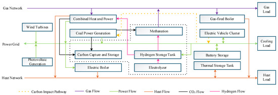
Figure 1.
Integrated Energy System Energy Flow Diagram (the black dotted box denotes the CCS–P2G conversion subsystem). To formulate the optimal scheduling model of the integrated energy system described above, this study develops detailed mathematical models for all devices in the system (see Appendix A). This section presents the virtual battery aggregation model for the EV cluster and the CHP–CCS–P2G coupling model that achieves coordinated carbon flows.
2.1. Cluster Electric Vehicle Model
- (1)
- Boundary model of a single EV
In a typical scenario, the feasible region model of a single EV is illustrated in Figure 2. and denote the time instants when the EV connects to and disconnects from the power grid, respectively. represents the initial energy of the EV upon grid connection. and refer to the lower and upper limits of the allowable energy level of the EV, while denotes the target energy expected to be achieved when the EV leaves the grid.
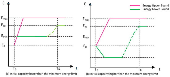
Figure 2.
Feasible region of a single EV.
For electric vehicles equipped with the V2G technology, their feasible power domain can be described by the upper and lower energy boundaries. The upper energy boundary corresponds to the trajectory when the EV starts charging at the maximum power immediately after connecting to the grid until the energy reaches the upper limit The lower boundary trajectory corresponds to the opposite process. When the initial energy of the connected EV is lower than the minimum allowable energy , the system first performs the charging operation until is reached, and then performs the discharging operation, as shown in Figure 2a. If the initial energy is higher than , the EV can directly participate in V2G operation, as shown in Figure 2b.
Figure 2a,b correspond to Equations (4)–(7), respectively, which describe the energy trajectories of EV:
where , and present the maximum and minimum energy levels of the i-th EV at time , respectively, while denotes the desired energy level expected by the vehicle owner when the EV leaves the grid. and denote the lower energy limits of the i-th EV, obtained, respectively, by backward deduction from the off-grid moment and forward deduction from the grid-connection moment. and indicate the maximum charging power and the maximum discharging power of the i-th EV, respectively. and represent, respectively, the minimum allowable energy of the -th EV and its initial energy at the grid-connection moment .
where and denote the upper and lower limits of the actual power of the -th EV at time t, respectively. represents the moment immediately before the off-grid time. and denote the maximum and minimum energy levels of the i-th EV at time , respectively.
Based on the above boundaries of power and energy, the state-of-charge equation for a single EV can be expressed as follows:
where denotes the power of the i-th EV at time t; and represent the energy of the i-th EV during the time interval . Both of them are decision variables.
- (2)
- Cluster EV Modeling Based on the Virtual Battery Model
A virtual battery model is adopted to characterize the flexibility of large-scale EV clusters in terms of charging and discharging [23]. The modeling approach relies on standardized parameters of an individual EV battery—such as capacity and charging/discharging power—together with representative travel patterns of users. By aggregating these characteristics, the collective energy and power boundaries of the EV cluster across different scheduling intervals can be derived.
where: and denote the upper and lower energy boundaries of the EV cluster at time t; and denote the upper and lower charging power boundaries of the EV cluster at time t; represents the number of EV connected to the grid at time t.
Since the total electric energy of the virtual battery model changes abruptly when the clustered electric vehicles connect to or disconnect from the grid, causing a step variation in energy, Equation (5) is modified accordingly for this model.
where represents the step change in the total energy of the virtual battery caused by the variation of the vehicle connection state between time t and t + 1. indicates that vehicle i is offline, and indicates that vehicle i is connected to the grid. Thus, When a vehicle switches from the off-grid state to the grid-connected state, a positive step change in energy is produced, equivalent to adding a fully charged vehicle to the system. In contrast, when the vehicle disconnects from the grid, a negative step change occurs, corresponding to a vehicle departing the cluster while carrying its remaining energy at the time of disconnection.
where: is the aggregated power of the EV cluster at time t; is the aggregated energy of the EV cluster at time t; denotes the net charging power of the EV cluster; denotes the net discharging power of the EV cluster; the maximum frequency regulation capacity available from the electric vehicle cluster at time t.
2.2. CHP-CCS-P2G Integrated Equipment Model
Following the modelling approach in Reference [24], the CHP unit is described by:
where: denotes the mixed gas power input to the CHP unit at time ; and are the electric and heat output of the CHP unit at time ; is the overall efficiency of the CHP unit, defined as the sum of the electric and thermal conversion efficiencies; and are the lower and upper bounds of the heat-to-electricity ratio; and denote the hydrogen and natural-gas input power to the CHP unit at time through hydrogen blending; and denote the lower heating values of hydrogen and methane, respectively; is the hydrogen blending ratio of the gas mixture at time ; is the carbon emission coefficient of methane combustion. is the lower heating value of the mixed fuel after hydrogen blending; and are the minimum and maximum electric power to ensure stable combustion in the gas turbine; and are the minimum and maximum thermal output of the waste heat boiler to maintain the required circulation flow.
The carbon flow process is formulated as follows:
where: denotes the CO2 emissions from the CHP system at time t; denotes the CO2 emissions from the GB; denotes the CO2 emissions from the CPG; represents the net CO2 directly discharged into the atmosphere; is the amount of CO2 captured by the CCS; is the amount of CO2 stored in geological storage at time t; is the CO2 utilized in the P2G process; defines the maximum safe capacity of the CO2 storage facility; is the power output of the coal-fired unit at time t; is its generation efficiency; is the carbon emission coefficient at time t; is the fuel energy input of the coal-fired unit at time t; and are the minimum and maximum power outputs of the coal-fired unit; and are the ramp-down and ramp-up limits of the coal-fired unit.
The electricity demand of the CCS system is composed of both basic consumption and operational consumption, which can be formulated as follows:
where: is the total power consumption of the CCS at time t; is the basic maintenance power consumption of the CCS; is the operating power consumption during the capture process; is the energy consumption intensity coefficient of the CCS; is the actual amount of CO2 captured at time t.
According to the chemical reaction equation of the second stage in the P2G device [20], the CO2 consumption in this stage can be expressed as:
where: is the density of CO2; is the gas volume generated by the MR at time t.
The mathematical model of the storage tank is given as follows:
where: denotes the solvent inventory of the rich tank at time t; denotes the solvent inventory of the lean tank at time t; represents the volumetric flow rate from the lean tank to the rich tank; represents the volumetric flow rate from the rich tank to the lean tank; and define the maximum allowable storage capacities of the lean and rich tanks, respectively; is the duration of one scheduling interval.
3. IES Stepwise Carbon Trading and Demand Response Model
3.1. Stepwise Carbon Trading Mechanism
- (1)
- Initial Carbon Emission Quota
In line with China’s carbon trading framework, the CHP units, GB, and coal-fired power plants are considered the primary participants in the quota allocation. The initial carbon emission quota for the IES can be formulated as:
where: , and represent the initial carbon emission allocations assigned to the coal-fired power plant, CHP units, and GB, respectively.
- (2)
- Actual Carbon Emissions
- (3)
- Carbon Trading Cost
The carbon trading cost can then be formulated as:
where denotes the growth ratio of the carbon trading price, is the initially specified benchmark carbon trading price, and represents the step length for partitioning the carbon emission intervals
3.2. Demand Response Model
This study incorporates both transferable and substitutable loads as demand-side flexibility resources to support demand response scheduling in the power system. The corresponding formulations are expressed as:
where: and represent the baseline electric and thermal loads before demand response, while and denote the adjusted loads after demand response. and correspond to the transferable electric and thermal loads within the scheduling horizon, whereas and indicate the curtailable portions. and describe the substitutable loads considered during scheduling.
- (1)
- Transferable Demand Response
The transferable load represents the temporal shifting of energy consumption, while the total transferable load over the scheduling horizon remains constant. During demand response, the adjustment in load—either increase or decrease—must not exceed the maximum regulation capacity. The transferable demand response constraint can be formulated as follows:
where: denotes the maximum transferable load allowed within the scheduling horizon of the system.
- (2)
- Curtailable Demand Response
Curtailable demand response relies on economic incentives to motivate users to curtail energy consumption during peak hours or emergency situations. This mechanism enhances system stability while offering financial compensation to participants. The corresponding constraint can be expressed as:
where: denotes the maximum curtailable load permitted within the scheduling horizon of the system.
- (3)
- Substitutable Demand Response
Substitutable demand response allows users to interchange different forms of energy within a given time frame. For example, during electricity price peaks, additional gas consumption can partially replace electricity usage without compromising the quality of energy services.
The corresponding constraint can be expressed as:
where: , represent the substitutable thermal and electric loads, respectively; is the coefficient defining the proportion of thermal load substitution; and specifies the maximum supply capacity of the power grid.
4. Low-Carbon Scheduling Model of the Park-Level Integrated Energy System
4.1. Objective Function
This paper constructs an optimal scheduling model for the IES that comprehensively considers economic, environmental, and reliability objectives. Beyond conventional cost components, the model explicitly accounts for EV smart charging strategies and battery degradation costs. A price-guided mechanism is designed to encourage EV to charge during renewable generation peaks and participate in V2G discharging during low-generation periods to provide ancillary services. In this way, renewable energy fluctuations can be mitigated, system flexibility can be improved, and simultaneously addresses battery aging concerns. The model aims to minimize the total system operating cost by coordinating the operating strategies of different energy units, thereby enabling an economically efficient and environmentally sound operation.
where: denotes the cost of carbon trading and carbon sequestration; denotes the operating cost of the coal-fired power generation unit; is the curtailment penalty cost; is the energy purchase cost; is the battery degradation cost; is the EV ancillary service revenue; is the smart charging reward; and is the off-peak discharging penalty.
where denotes the frequency regulation capacity provided in period t; denotes the real-time electricity price in period t; and is the calling coefficient, which is set to 0.2 [25,26]
where: and denote the coefficients for charging incentives and discharging penalties, respectively; and represent the forecasted wind and PV outputs in period t; while and correspond to the charging and discharging power of EV during period t.
where: denotes the penalty coefficient applied to renewable curtailment; and represent the curtailed wind and PV energy during period t, respectively. represents the curtailed wind power at time t, and represents the curtailed photovoltaic power at time t.
where: denotes the fixed startup and shutdown cost of the unit; and indicate the on/off status of the unit in period t; is the coal price; represents the coal consumption in period t; is the operation and maintenance cost coefficient of the unit; and denotes the output power of the coal-fired generating unit in period t.
where: is the unit price of CO2 sequestration; denotes the mass of CO2 stored at time t; and refers to the carbon trading cost incurred during period t.
where: denotes the degradation cost coefficient of the battery, and indicates the discharge energy of the EV cluster during period t.
where: denotes the unit price of natural gas, and corresponds to the amount of natural gas purchased during period t.
4.2. Energy Balance Constraints
The supply–demand balance of the system primarily includes the electricity, heat, and gas loads.
The electricity balance is expressed as:
The heat load balance is expressed as:
The gas load balance is expressed as:
5. Uncertainty of Wind and Solar Power and Scenario Reduction
Due to the inherent uncertainty of wind and photovoltaic outputs, this study employs the Monte Carlo sampling method to generate scenario sets of wind–PV power generation. The normalized outputs of wind and photovoltaic power at time interval t are denoted by the random variables and . Their probability distributions are derived by fitting historical measurement data. During the scheduling horizon, wind power is assumed to follow a Weibull distribution, while photovoltaic power is modeled by a Beta distribution:
In this formulation, K and C are the shape and scale parameters of the Weibull distribution, while and are the parameters of the Beta distribution, with representing the Beta function.
Given the prescribed probability distributions, Monte Carlo sampling is used to generate joint wind–PV scenarios.
Here, and denote the wind and photovoltaic output sequences for scenario n across the scheduling horizon T, while is the occurrence probability of scenario n, typically assigned as .
To reduce the complexity of the subsequent optimization model, a fast backward scenario reduction method is applied to the original scenario set. From the set of N original scenarios, representative scenarios are selected to form the subset which is used as the reduced scenario set:
In this formulation, represents the probability weight of scenario k, which satisfies the normalization condition:
The purpose of scenario reduction is to retain the statistical characteristics of the original scenario set as faithfully as possible. This process is mathematically formulated as minimizing the weighted distance between the original and the reduced representative scenarios:
Here, denotes the distance measure between scenarios i and j. The Euclidean distance is adopted in this study to quantify the dissimilarities in wind and photovoltaic power outputs.
The scenario reduction decreases the number of scenarios from N to K, preserving representativeness and diversity while reducing computational complexity.
For further simplification, the K scenarios are aggregated into one expected scenario by probability weighting, with wind and photovoltaic outputs given as:
The expected scenario represents the average wind–solar output and is applied for system analysis and strategy comparison.
6. Case Study Analysis
6.1. Basic Data
A typical industrial park in northern China is selected as the study system, and numerical simulations are performed on this system. In this case study, fuel prices, carbon trading prices, start-up and shut-down costs, and other key parameters are mainly taken from References [27,28,29], so that the input data remain reasonable and representative. Based on measured wind and PV data from a specific region, the uncertainty treatment method proposed in Section 4 is applied to generate 1000 wind–PV output scenarios and the corresponding reduced scenario set, as illustrated in Figure 3, Figure 4 and Figure 5. The main operating parameters of the devices in the integrated energy system are summarized in Table 1 and Table 2.
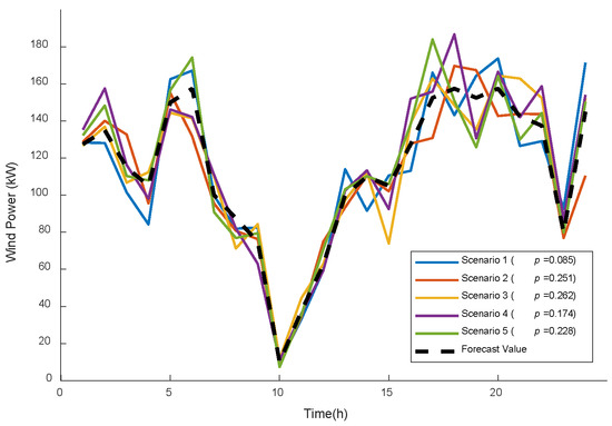
Figure 3.
Wind Power Generation Forecast Data.
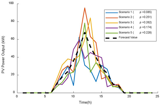
Figure 4.
Photovoltaic Power Generation Forecast Data.
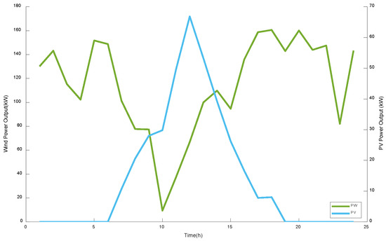
Figure 5.
Final Power Generation Forecast Data.

Table 1.
Design Parameters.
Table 2.
Key model parameters and their values.
6.2. Verification of Low-Carbon Economic Dispatch Benefits in the Integrated Energy System
To comprehensively assess the effects of various low-carbon technology pathways on the operational performance of the integrated energy system, three typical scenarios are designed for comparative analysis. Scenario 1 represents the baseline system without P2G, CCS, or electric vehicles. Scenario 2 integrates P2G and CCS technologies to enhance renewable energy utilization and reduce carbon emissions. Scenario 3 further incorporates electric vehicle clusters on the basis of Scenario 2, exploiting their bidirectional regulation capability to improve system flexibility. The operating cost and carbon emission levels of the three scenarios are evaluated using the proposed model, as summarized in Table 3, to verify the economic and environmental benefits of different low-carbon strategies and to highlight the advantages of the integrated energy system in low-carbon economic dispatch.
Table 3.
Operating Cost Comparison for Different System Setups.
According to Table 3, Scenario 1 (baseline) incurs the highest total cost of 1.9574 million CNY, dominated by coal-fired generation (0.4216 million CNY) and natural gas purchases (1.1189 million CNY). The carbon trading cost also reaches 0.2840 million CNY, underscoring the system’s heavy reliance on fossil fuels and revealing that both emissions and external energy expenditures are major constraints on economic and low-carbon performance.
In Scenario 2, the adoption of P2G and CCS reduces the total cost to 1.7119 million CNY, 12.5% lower than the baseline. Specifically, carbon trading and sequestration expenses fall by 46.3%, coal-fired generation costs by 17.2%, and gas purchases by 3.3%. These results indicate that P2G primarily improves renewable energy utilization, thereby lowering gas demand, while CCS effectively curbs emissions and relieves carbon trading pressure. The synergy between the two technologies achieves dual benefits in economic performance and carbon reduction, offering a more robust optimization pathway for system operation.
Furthermore, in Scenario 3, the integration of the electric vehicle (EV) cluster further reduced the total system cost to 1.6221 million CNY, representing a 5.2% decrease compared with Scenario II. Among the cost components, the coal-fired unit cost declined to 0.2892 million CNY, and the gas purchase cost decreased to 1.0393 million CNY, corresponding to reductions of 17.1% and 4.0%, respectively. The bidirectional regulation capability of electric vehicles enables them to absorb electricity during off-peak periods and discharge during peak periods, which not only effectively mitigates peak loads and alleviates the ramping pressure of generation units but also reduces gas consumption, thereby further enhancing the system’s economic efficiency and operational flexibility. In addition, the battery degradation cost was 0.0111 million CNY, while the V2G ancillary service revenue reached 0.0101 million CNY; the two values were nearly offset, indicating that EV participation enhances system flexibility without imposing significant additional economic burden. Meanwhile, the carbon trading and sequestration cost in Scenario 3 increased to 0.2061 million CNY compared with Scenario 2. This is mainly attributed to the smoother system load profile after EV integration, which enables the CCS system to operate at higher loading levels and for longer durations, thereby capturing and storing more CO2 and increasing sequestration expenditures. Nevertheless, the total cost in Scenario III remains the lowest among all three scenarios, clearly demonstrating the comprehensive advantages of EVs and the P2G–CCS pathway in promoting low-carbon energy transition, reducing fossil-fuel dependence, and enhancing operational flexibility within the integrated energy system.
6.3. Simulation of Optimal System Operation
To further analyze the operational features of the integrated energy system on a typical day, Figure 6, Figure 7, Figure 8 and Figure 9 depict the energy balances of electricity, heat, gas, and hydrogen. The results confirm that multi-energy coupling and coordinated scheduling enable effective supply–demand matching and smooth energy conversion.
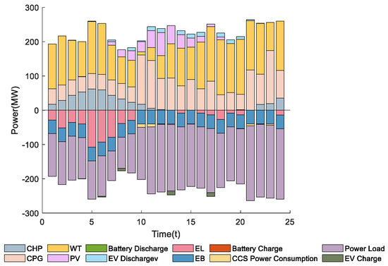
Figure 6.
Electrical Energy Balance Diagram.
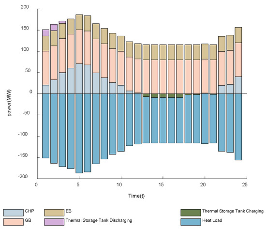
Figure 7.
Thermal Energy Balance Diagram.
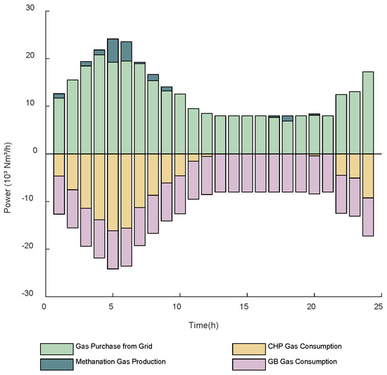
Figure 8.
Gas Energy Balance Diagram.
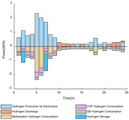
Figure 9.
Hydrogen Energy Balance Diagram.
As shown in Figure 6, the P2G unit primarily operates between 00:00–09:00, when electricity demand is low. During this period, surplus electricity is converted into natural gas and hydrogen, lowering purchase costs while providing gaseous reserves for subsequent peak periods. Coal-fired generation decreases when wind output is high, whereas during 22:00–10:00, when wind and PV are limited, it jointly supplies power with CHP. The discharging of electric vehicles mainly occurs between 11:00–20:00, whereas charging is observed around 8:00, 13:00, and 17:00. This pattern arises because the electrical load reaches its peak from afternoon to evening, when the system experiences higher supply pressure; EV discharging during this period effectively mitigates peak power shortages and reduces operational costs. In contrast, during morning and midday hours with sufficient photovoltaic generation or lower electricity prices, EVs tend to charge, absorbing surplus renewable energy and thereby strengthening the system’s peak-shaving and valley-filling capability. Because it is more economical to use P2G and EV clusters for flexibility, the battery storage unit remains idle
Figure 7 presents the thermal power balance of the system. The heat load is mainly covered by CHP, EB, and GB units, while thermal storage provides supplementary output when demand exceeds generation capacity. The adopted operation strategy, characterized by nighttime discharging and midday charging, mitigates peak stress on primary equipment and improves the overall efficiency of energy utilization.
Figure 8 depicts the gas power balance of the system, highlighting the scheduling of natural gas. A considerable share of natural gas is procured externally to meet the requirements of CHP, GT, and GB units. The CH4 generated via P2G partially offsets this demand and thereby reduces gas purchase costs. Coordinated operation among system units enables low-carbon and economically efficient performance.
Figure 9 illustrates the hydrogen energy balance, indicating that the hydrogen consumed by the methanation reactor, gas boiler, and combined heat and power (CHP) unit is produced via water electrolysis. The hydrogen storage tank acts as a buffer to absorb or release hydrogen at different time periods. During the early hours of low load and electricity price, the system mainly performs hydrogen production and storage. From noon to evening, hydrogen production and consumption remain roughly balanced, reflecting the operation of hydrogen blending in the gas network. At night and around peak-demand periods, methanation and hydrogen blending demand increase, and the hydrogen storage shifts from charging to discharging to support hydrogen utilization. This sequential transition of “production–storage–utilization” enables cross-period energy transfer and contributes to peak shaving and valley filling: on one hand, it provides a stable hydrogen source for CO2 methanation and reduces dependence on external natural gas purchases; on the other hand, it enhances renewable energy utilization and promotes low-carbon operation of the integrated energy system.
6.4. EV Charging/Discharging Profiles, SOC Regulation, and Frequency Response
To investigate the charging and discharging behavior of the electric vehicle cluster under typical wind–solar generation scenarios, the 24 h profiles of charging/discharging power and state of energy are extracted from the simulation results of the proposed optimal scheduling model. Figure 10 illustrates the asymmetric charging and discharging pattern of EV clusters under the V2G mode. The charging power is 33.28 MW, whereas the discharging power reaches 111.34 MW, which is 3.31 times higher. The strategy tends to provide high-power discharging support during periods of high electricity prices. This “shallow charging and deep discharging” pattern enables EVs to play a critical role in peak shaving and valley filling. Notably, during price peaks, discharging power rises rapidly to 9.36 MW with a response rate exceeding 4.02 MW/h, demonstrating strong responsiveness to market signals. According to the calculated data, the dynamic available capacity of the electric vehicle (EV) cluster fluctuates throughout the day, with an average upper limit of 69.6 MWh and an average lower limit of 24.2 MWh. Considering only the effective periods when the available capacity is greater than zero, the average SOC utilization rate is approximately 46%, indicating that the system retains about 54% of redundant margin to cope with uncertainties while maintaining scheduling flexibility. In addition, the actual energy in certain time periods approaches the upper and lower capacity limits, suggesting that the operational strategy has sufficient capability for both energy release and absorption under extreme conditions, whereas during most periods it remains at the mid-level range of the capacity interval, achieving a balance between economic efficiency and operational security.
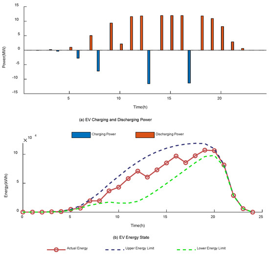
Figure 10.
Electric Vehicle Charging/Discharging Power and SOC Status Diagram.
Further observation of temporal characteristics reveals that EV charging demand is concentrated during early morning and forenoon valley periods, where charging power rises markedly to replenish vehicle energy and absorb low-cost electricity. Conversely, during morning peaks, midday, and evening high-load periods, discharging power increases rapidly, indicating that EVs undertake large-scale reverse supply during peak hours. The SOC curve fluctuates within the mid-range between upper and lower bounds, ensuring both scheduling flexibility and redundancy to accommodate renewable variability and sudden load changes. Overall, EV clusters exhibit a pattern of “valley charging and peak discharging,” aligning well with the objective of peak shaving and valley filling.
Figure 11 illustrates the dynamic relationship between the regulation capacity of EV clusters and electricity prices. Regulation capacity strongly correlates with price trends: it rises sharply during price increases and stabilizes at 5–6 MW when prices remain high, highlighting the high sensitivity of V2G clusters to market signals. During low-price periods, the capacity nearly falls to zero as the system actively preserves reserves, whereas during peak-price hours, the capacity approaches its maximum, indicating full deployment of flexibility resources for maximum revenue. Notably, between 14:00 and 18:00, the regulation capacity reaches saturation without further increase, reflecting the physical power boundary constraints of the system.
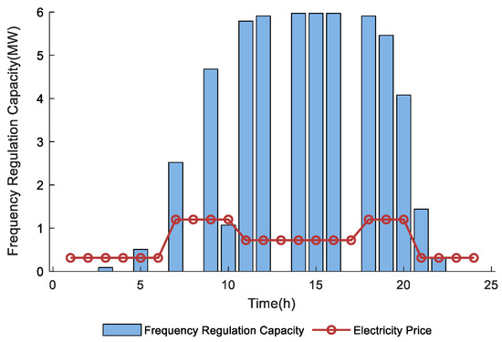
Figure 11.
V2G Frequency Regulation Capacity.
Overall, the electric vehicle (EV) cluster operating under the V2G mode demonstrates not only high efficiency in economic response but also a strong correlation between discharging power and electricity price peaks. It responds rapidly, effectively participating in market peak shaving while serving as a reliable capacity reserve. Meanwhile, it maintains economic performance by retaining a considerable SOC margin to ensure system security. Therefore, the introduction of the EV cluster serves as a high-value and high-reliability flexible regulation core, playing a crucial role in alleviating peak–valley contradictions and enhancing renewable energy consumption.
6.5. Synergistic Benefits of EV Charging with Wind–Solar Generation and Market Prices
Figure 12 illustrates the variations in electric vehicle charging power along with wind power, photovoltaic generation, and electricity price.
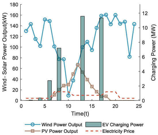
Figure 12.
Coordination Diagram of EV Charging and Renewable Power Output.
As illustrated in Figure 12, the charging behavior of electric vehicles is highly correlated with the temporal patterns of wind and solar generation. Specifically, between 10:00 and 15:00, when photovoltaic output increases rapidly and remains high, EV charging power rises accordingly, effectively absorbing surplus renewable energy. During nighttime hours with limited solar output, the availability of wind generation enables EVs to maintain a certain level of charging load, indicating efficient utilization of wind energy. These results suggest that, under the proposed scheduling strategy, EVs tend to charge primarily during renewable-abundant periods, thereby enhancing wind–solar energy utilization. Moreover, when the electricity price increases between 17:00 and 21:00 and solar generation is unavailable, EV charging power declines significantly or even halts. This implies that EV charging behavior is jointly influenced by renewable generation and price signals—charging demand is released during low-price periods and suppressed during high-price hours, thus mitigating the system’s economic burden during expensive intervals.
In summary, Figure 12 illustrates that, in the charging scheduling process, electric vehicles promote efficient renewable-energy utilization by concentrating their charging activities within periods of high wind and photovoltaic generation. On the other hand, guided by electricity price signals, electric vehicles (EVs) reduce charging demand during high-price periods, thereby optimizing the system’s economic performance. Therefore, EVs act not only as important load units that promote renewable energy utilization but also as flexible regulating resources capable of responding effectively to market price signals.
7. Sensitivity Analysis
To quantify how the EV scheduling scale influences multi-agent low-carbon economic dispatch in the integrated energy system, the system performance with 1500 to 2500 participating EVs is further compared, as shown in Figure 13.
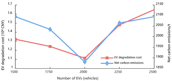
Figure 13.
Impact of different EV fleet sizes on optimal scheduling.
As shown in Figure 13, when the number of EVs increases from 1500 to 2000, the larger fleet scale enhances the regulation capability of the integrated energy system. On the one hand, EVs charge during load valleys to absorb surplus renewable energy and discharge during peak periods to replace high-carbon generation, which effectively reduces system-level carbon emissions. On the other hand, the revenue from V2G ancillary services increases markedly and offsets the battery degradation cost, thereby improving both the low-carbon performance and the economic performance of the system. When the number of EVs is further increased to 2500, the aggregate charging power of the EV fleet exceeds the renewable absorption capability of the system in certain periods. To satisfy this large scheduling requirement, the system has to dispatch conventional units with higher marginal carbon intensity, which induces additional indirect carbon emissions. At the same time, market saturation reduces the average V2G revenue, whereas deeper discharging further accelerates battery degradation. Therefore, an EV population of around 2000 constitutes a near-optimal scale range for this system: it maintains system flexibility and renewable energy absorption while achieving a joint optimum between EV degradation cost and net CO2 emissions.
8. Conclusions and Future Work
- (1)
- This paper develops a low-carbon economic dispatch model for a park-level integrated energy system that includes the coordinated operation of an electric vehicle (EV) cluster and a P2G–CCS scheme, and conducts quantitative comparative analysis of simulation results under multiple scenarios to obtain the following conclusions and outlook. Battery degradation and economic balance: During charging and discharging, EVs inevitably incur battery degradation cost. Simulation results indicate that the revenue from V2G ancillary services can offset about 91% of this degradation cost, keeping the net loss due to degradation at a very small and acceptable level. Although the degradation cost is not fully offset, its impact on the overall economic performance of the system is limited and does not reduce the value of EVs as flexible regulation resources.
- (2)
- System operation and flexibility improvement: By using a virtual-battery aggregation model, dispersed EVs are represented as a controllable aggregate capacity, which allows frequency regulation capacity constraints to be scheduled directly at the system level and, together with P2G–CCS, to form a coupling path from flexibility to renewable energy absorption and further to emission reduction. With the model size kept within a controllable range, this framework improves the system response speed, power regulation capability, and low-carbon economic performance. Case studies indicate that, compared with Scenario 2 without EVs, the participation of EVs in Scenario 3 further reduces the total system cost by 5.2% and exhibits a strong peak-shaving and valley-filling capability.
- (3)
- Low-carbon performance and integrated benefits improvement: By introducing P2G–CCS units and coordinating them with EVs, the system not only achieves efficient utilization of renewable electricity during surplus periods but also reduces its dependence on external gas purchases and significantly lowers carbon emissions. Compared with Scenario 2, the coordinated scheduling scheme that combines EVs with P2G–CCS reduces the system gas purchase cost by 4.0% and exhibits clear advantages in both operating cost and environmental performance, indicating good feasibility and development potential under low-carbon economic objectives.
- (4)
- This study builds a virtual-battery-based scheduling framework for EV clusters and represents battery degradation cost with a linearized model, which cannot fully capture the complex impacts of SOC and charge/discharge current on battery degradation. Future work will focus on developing a nonlinear degradation model that balances accuracy and computational efficiency. In addition, the study scope will be extended from park-level coordination to the regional level by coupling real-time electricity price signals with energy pipeline facilities, so as to achieve coordinated optimization of markets, technologies, and infrastructures.
Author Contributions
J.G.: Conceptualization, Methodology, Software, Formal analysis, Writing—original draft; W.H.: Data curation, Validation, Visualization; C.Y.: Investigation, Resources, Validation; K.F.: Supervision, Conceptualization, Methodology, Writing—review and editing. All authors have read and agreed to the published version of the manuscript.
Funding
This study was supported by the Science and Technology Project of State Grid East China Branch (Project No.H2021-111). The sponsor only provides financial support. The funder was not involved in the study design, collection, analysis, interpretation of data, the writing of this article, or the decision to submit it for publication.
Data Availability Statement
The data presented in this study are not publicly available due to privacy restrictions. Data may be made available upon reasonable request from the corresponding author.
Conflicts of Interest
The authors declare no conflicts of interest.
Appendix A
Appendix A.1. Formatting of Mathematical Components
In the P2G module, the Electrolyzer (EL) produces hydrogen through water electrolysis, while the Hydrogen Storage Tank (HST) stores the generated hydrogen for subsequent use. The Methanation Reactor (MR) captures CO2 from CHP units, coal-fired units, or gas boilers and converts it into methane, which is injected into the upper gas network to improve system profitability and reduce energy waste. Moreover, by mitigating the intermittency and storage constraints of renewable power, the P2G system effectively enhances renewable energy utilization within the integrated energy system [30,31].
- (1)
- EL Model
- (2)
- Storage Tank Model
- (3)
- MR Model
Appendix A.2. Electric Boiler Model
The operation of the EB can be formulated as:
where: represents the effective thermal output of the EB under nominal operating conditions; denotes the conversion efficiency between electrical input and thermal output; is the electrical input of the EB at time t; and specify the lower and upper bounds of electric input required to sustain normal circulation of the boiler system; and define the minimum and maximum permissible ramping rates to ensure safe operation.
Appendix A.3. Gas-Fired Boiler Model
The GB model is given as:
where: is denotes the mixed-gas power input to the gas-fired boiler at time t; denotes the lower heating value of the mixed gas after blending hydrogen with natural gas; denotes the hydrogen input power to the GB unit at time t through hydrogen blending; is the hydrogen blending ratio of the gas in period t; denotes the natural-gas input power to the GB unit at time t through hydrogen blending; and are the minimum and maximum stable outputs of the GB.
References
- Peng, K.; Feng, K.; Chen, B.; Shan, Y.; Zhang, N.; Wang, P.; Fang, K.; Bai, Y.; Zou, X.; Wei, W.; et al. The global power sector’s low-carbon transition may enhance sustainable development goal achievement. Nat. Commun. 2023, 14, 3144. [Google Scholar] [CrossRef]
- Möller, T.; Högner, A.E.; Schleussner, C.-F.; Bien, S.; Kitzmann, N.H.; Lamboll, R.D.; Rogelj, J.; Donges, J.F.; Rockström, J.; Wunderling, N. Achieving net zero greenhouse gas emissions critical to limit climate tipping risks. Nat. Commun. 2024, 15, 6192. [Google Scholar] [CrossRef]
- Yan, R.; Wang, J.; Huo, S.; Qin, Y.; Zhang, J.; Tang, S.; Wang, Y.; Liu, Y.; Zhou, L. Flexibility improvement and stochastic multi-scenario hybrid optimization for an integrated energy system with high-proportion renewable energy. Energy 2023, 263, 125779. [Google Scholar] [CrossRef]
- Hinkelman, K.; Garcia, J.D.F.; Anbarasu, S.; Zuo, W. A Review of Multi-Energy Systems from Resiliency and Equity Perspectives. Energies 2025, 18, 4536. [Google Scholar] [CrossRef]
- Mancò, G.; Tesio, U.; Guelpa, E.; Verda, V. A review on multi energy systems modelling and optimization. Appl. Therm. Eng. 2024, 236, 121871. [Google Scholar] [CrossRef]
- Khou, S.A.; Olamaei, J.; Hosseini, M.H. Strategic scheduling of the electric vehicle-based microgrids under the enhanced particle swarm optimization algorithm. Sci. Rep. 2024, 14, 30795. [Google Scholar] [CrossRef] [PubMed]
- Wu, J.; Cheng, X.; Huang, H.; Fang, C.; Zhang, L.; Zhao, X.; Zhang, L.; Xing, J. Remaining useful life prediction of Lithium-ion batteries based on PSO-RF algorithm. Front. Energy Res. 2023, 10, 937035. [Google Scholar] [CrossRef]
- Mao, Y.; Cai, Z.; Jiao, X.; Long, D. Multi-timescale optimization scheduling of integrated energy systems oriented towards generalized energy storage services. Sci. Rep. 2025, 15, 8549. [Google Scholar] [CrossRef] [PubMed]
- Liu, Z.-F.; Liu, Y.-Y.; Jia, H.-J.; Jin, X.-L.; Liu, T.-H.; Wu, Y.-Z. Bi-level energy co-optimization of regional integrated energy system with electric vehicle to generalized-energy conversion framework and flexible hydrogen-blended gas strategy. Appl. Energy 2025, 390, 125868. [Google Scholar] [CrossRef]
- Jia, S.; Kang, X.; Cui, J.; Tian, B.; Xiao, S. Hierarchical stochastic optimal scheduling of electric thermal hydrogen integrated energy system considering electric vehicles. Energies 2022, 15, 5509. [Google Scholar] [CrossRef]
- Wang, Z.; Li, J.; Li, P.; Zhang, H.; Jurasz, J.; Wang, L.; Li, J.; Zheng, W. A comparative study on the performance of hybrid energy storage with electric vehicles and batteries in integrated energy system. J. Energy Storage 2025, 114, 115791. [Google Scholar] [CrossRef]
- Sagaria, S.; van der Kam, M.; Boström, T. Vehicle-to-grid impact on battery degradation and estimation of V2G economic compensation. Appl. Energy 2025, 377, 124546. [Google Scholar] [CrossRef]
- van der Zwaan, B.; Fattahi, A.; Longa, F.D.; Dekker, M.; van Vuuren, D.; Pietzcker, R.; Rodrigues, R.; Schreyer, F.; Huppmann, D.; Emmerling, J.; et al. Electricity- and hydrogen-driven energy system sector-coupling in net-zero CO2 emission pathways. Nat. Commun. 2025, 16, 1368. [Google Scholar] [CrossRef]
- Li, Y.; Zhang, F.; Li, Y.; Wang, Y. An improved two-stage robust optimization model for CCHP-P2G microgrid system considering multi-energy operation under wind power outputs uncertainties. Energy 2021, 223, 120048. [Google Scholar] [CrossRef]
- Marzi, E.; Morini, M.; Saletti, C.; Vouros, S.; Zaccaria, V.; Kyprianidis, K.; Gambarotta, A. Power-to-Gas for energy system flexibility under uncertainty in demand, production and price. Energy 2023, 284, 129212. [Google Scholar] [CrossRef]
- Faramarzi, H.; Ghaffarzadeh, N.; Shahnia, F. A new stochastic multi-objective model for the optimal management of a PV/wind integrated energy system with demand response, P2G, and energy storage devices. Front. Energy Res. 2025, 13, 1537703. [Google Scholar] [CrossRef]
- Wang, Y.; Zhou, Y. Equipment capacity matching methodology and techno-economic analysis for a novel low-carbon multi-energy system with the integration of oxy-coal combustion power plant and power-to-gas. Energy 2025, 322, 135693. [Google Scholar] [CrossRef]
- Pan, C.; Jin, T.; Li, N.; Wang, G.; Hou, X.; Gu, Y. Multi-objective and two-stage optimization study of integrated energy systems considering P2G and integrated demand responses. Energy 2023, 270, 126846. [Google Scholar] [CrossRef]
- Chen, L.; Liu, K.; Zhao, K.; Hu, L.; Liu, Z. Optimal scheduling of electricity-hydrogen-thermal integrated energy system with P2G for source-load coordination under carbon market environment. Energy Rep. 2025, 13, 2269–2276. [Google Scholar] [CrossRef]
- Yang, C.; Dong, X.; Wang, G.; Lv, D.; Gu, R.; Lei, Y. Low-carbon economic dispatch of integrated energy system with CCS-P2G-CHP. Energy Rep. 2024, 12, 42–51. [Google Scholar] [CrossRef]
- Huang, X.; Zhong, J.; Xiao, M.; Zhu, Y.; Zheng, H.; Zheng, B. Optimal and Sustainable Scheduling of Integrated Energy System Coupled with CCS-P2G and Waste-to-Energy Under the “Green-Carbon” Offset Mechanism. Sustainability 2025, 17, 4873. [Google Scholar] [CrossRef]
- Sattar, M.; Moghaddam, M.S.; Azarfar, A.; Salehi, N.; Vahedi, M. Co-optimization of integrated energy systems in the presence of renewable energy, electric vehicles, power-to-gas systems and energy storage systems with demand-side management. Clean Energy 2023, 7, 426–435. [Google Scholar] [CrossRef]
- Izadkhast, S.; García-González, P.; Frías, P. An aggregate model of plug-in electric vehicles for primary frequency control. IEEE Trans. Power Syst. 2015, 30, 1475–1482. [Google Scholar] [CrossRef]
- Zheng, Z.; Xiwang, A.; Sun, Y. Optimal Scheduling of Integrated Energy System Considering Hydrogen Blending Gas and Demand Response. Energies 2024, 17, 1902. [Google Scholar] [CrossRef]
- Zhou, C.; Xiang, Y.; Zhang, X.; Zhang, S.; Liu, Y.; Liu, J.; Hu, S. Regulation Potential and Economic Analysis of V2G Ancillary Services: A Case Study of Shanghai. Electr. Power Autom. Equip. 2021, 41, 135–141. (In Chinese) [Google Scholar] [CrossRef]
- Lu, L.; Wen, F.; Xue, Y.; Kang, J. Economic Analysis of Ancillary Services Provided by Electric Vehicles. Autom. Electr. Power Syst. 2013, 37, 43–49+58. (In Chinese) [Google Scholar]
- China Coal Market Network. China Coal Market Network EB/OL. Available online: https://www.cctd.com.cn/ (accessed on 25 May 2024).
- Chen, D.; Liu, F.; Liu, S. Optimal Scheduling of a Virtual Power Plant with P2G–CCS Coupling and Hydrogen-Blended Gas Units under Stepwise Carbon Trading. Power Syst. Technol. 2022, 46, 2042–2054. (In Chinese) [Google Scholar] [CrossRef]
- Sun, H.; Duan, J. Optimal Scheduling of an Integrated Energy System with Oxy-Fuel Combustion Power Plants and Hydrogen-Blended Gas Equipment. Therm. Power Gener. 2025, 54, 78–87. (In Chinese) [Google Scholar] [CrossRef]
- Yu, K.; Son, P.V. Review of trans-Mediterranean power grid interconnection: A regional roadmap towards energy sector decarbonization. Glob. Energy Interconnect. 2023, 6, 115–126. [Google Scholar] [CrossRef]
- Xu, M.; Zhao, D.; Yu, C.; Zhang, S.; Wan, J.; Li, W.; Liu, H. Research on the optimal scheduling strategy of the integrated energy system of electricity to hydrogen under the stepped carbon trading mechanism. Front. Energy Res. 2024, 12, 1410120. [Google Scholar] [CrossRef]
Disclaimer/Publisher’s Note: The statements, opinions and data contained in all publications are solely those of the individual author(s) and contributor(s) and not of MDPI and/or the editor(s). MDPI and/or the editor(s) disclaim responsibility for any injury to people or property resulting from any ideas, methods, instructions or products referred to in the content. |
© 2025 by the authors. Licensee MDPI, Basel, Switzerland. This article is an open access article distributed under the terms and conditions of the Creative Commons Attribution (CC BY) license (https://creativecommons.org/licenses/by/4.0/).