Abstract
This paper presents a Prescribed Performance Control (PPC) approach for robotic systems experiencing communication delay and disturbances. Under input and feedback delays, a state feedback controller is designed to maintain the output tracking error within prescribed performance specifications. Additionally, a super-twisting algorithm-based sliding-mode observer is proposed to estimate and compensate for external disturbance in the robotic system. Based on the Lyapunov method, appropriate controller parameters and observer gains are selected to ensure the accuracy of output tracking and disturbance estimation. Finally, the effectiveness of the proposed approach is validated through simulations on a nonlinear robotic system. The proposed method remains effective in the simultaneous presence of state measurement delay, control input delay, and disturbance.
1. Introduction
Robotic manipulators have emerged as indispensable tools across a wide spectrum of modern industrial applications. In practical implementations, time delays frequently arise due to the inherent communication latency between control systems and robotic actuators. Consequently, investigating predictive control strategies for robotic manipulators under time delay conditions presents substantial practical significance and research value [1].
Network-induced time delays can significantly degrade the performance of robotic systems, potentially leading to instability. Research in this domain has predominantly focused on mitigating delays in control inputs [2,3,4,5,6,7,8,9,10,11]. A subset of studies is dedicated to state measurement delays [12,13,14], while a smaller body of literature concurrently addresses both types [15,16,17]. However, the predominant focus of existing research has been on ensuring system stability, often with less emphasis on performance metrics.
Evaluating system performance in the context of concurrent control input and state measurement delays continues to be a focal point of contemporary research. Although Model Predictive Control (MPC) incorporates performance metrics [18], its practical application is often hindered by a strong reliance on a precise system model. To overcome the challenge of model uncertainty, methodologies like Prescribed Performance Control (PPC) have been developed for nonlinear systems [19,20]. Nevertheless, a practical limitation of these approaches is their requirement for high-order derivatives of the reference trajectory. Furthermore, their scope is typically restricted to addressing control input delays, leaving state measurement delays unaccounted for.
The existing literature on Prescribed Performance Control (PPC) for robotic systems has not adequately addressed the impact of external disturbances, which poses a significant threat to system stability. To circumvent the lack of end-effector force sensors in many robotic platforms, the method proposed by Ficuciello et al. [21] utilizes force estimation; however, its effectiveness is limited by its reliance on an open-loop estimator that is highly susceptible to noise. In contrast, the disturbance observer represents a well-established alternative for estimating external forces in robotic systems [22,23,24]. For instance, Liu et al. [25] constructed a globally and exponentially stable joint torque observer using only position measurements. Similarly, other researchers have utilized neural networks to develop external force estimators [26,27]. The method by [28] employs reinforcement learning algorithms to address the challenge of unpredictable disturbances in changing environments.
This paper designs a state feedback controller in the presence of a communication delay and disturbance, which is used to keep the output tracking error within the specified performance range. A super-twisting algorithm-based sliding-mode observer is proposed to estimate and compensate for external disturbance in the robotic system. The parameters are selected and adjusted based on the Lyapunov theory. Finally, simulation verification was carried out on a two-degree-of-freedom robotic system.
This paper’s main contributions and innovations include the following:
- This paper introduces a novel PPC method to maintain the tracking performance of a robot system under state measurement delays, control input delays, and external disturbances.
- An integrated super-twisting disturbance observer was designed, which provides accurate and real-time estimates of external disturbances, thereby significantly enhancing the system’s overall robustness.
The rest of this article is organized as follows: Section 2 presents the dynamic model of the robotic system. Then, it details the design of the proposed controller and disturbance observer. After that, a stability analysis is conducted on the closed-loop system. In Section 3, simulation studies are conducted to validate the theoretical findings and demonstrate the effectiveness of the proposed method. Finally, Section 4 concludes the paper with a summary of the key contributions.
2. Materials and Methods
2.1. Dynamic Model of Robotic System
The dynamics of an n-DOF robotic manipulator, subject to external disturbance, can be expressed as follows:
where and , respectively, denote the joint angles and angular velocities of the robotic manipulator, represents a symmetric positive definite inertia matrix, is the matrix of the centripetal and Coriolis torques, represents the vector of gravitational torques, F denotes input torques, and d is an externally applied disturbance.
Denote . The state space model of system (1) can be described by
where represents the system state, , , and .
Prescribed Performance Control constrains the system tracking error to remain within predefined, time-varying boundaries. These boundaries are delineated by a performance function, which explicitly specifies key performance metrics such as the maximum allowable steady-state error and the minimum convergence rate. The proposed controller is developed for the Prescribed Performance Control problem in the presence of concurrent time delays and external disturbances. This study considers the system described in (2), which is subject to a desired trajectory , a state measurement delay , and a control input delay . A state feedback controller is designed to achieve the following objectives:
- The system output is required to track the desired trajectory in accordance with prescribed performance specifications, namely, the maximum steady-state error and the minimum convergence rate.
- A disturbance observer is designed to compensate for the external disturbances inherent in practical robotic applications.
The structure of the closed-loop system is shown in Figure 1.
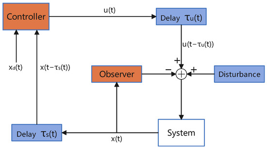
Figure 1.
Closed-loop system schematic diagram.
Our work is based on the following assumptions:
Assumption 1.
The communication delays and are assumed to be bounded and continuously differentiable. Furthermore, is assumed to be known, whereas is unknown but upper-bounded by a positive constant . Their derivatives are bounded, satisfying and . Moreover, there exist positive constants and such that for all , the inequality is satisfied.
Remark 1.
By comparing the timestamp of the generated data and the timestamp of the data reaching the controller, the state measurement delay can be estimated relatively accurately. The control input delay is generally impossible to measure. Therefore, this is why it is assumed that is known, while is unknown. The derivative of the time delay being less than 1 is a condition for the stability of the system. In this case, the system is still capable of “catching up” with the delay. If the derivative of the delay is greater than 1, it indicates that the growth rate of the delay is faster than the rate of time passage. This causes the control system to violate the law of causality to some extent.
Assumption 2.
The components of the desired trajectory, for , are known and belong to the interval . Furthermore, these trajectory components are bounded, i.e., .
Assumption 3.
The disturbance d and its time derivative are bounded.
2.2. Controller Design
2.2.1. Design of the Controller
The design of the proposed controller builds upon the framework presented in [14]. Let be a strictly increasing function that satisfies the limit conditions and . For notational simplicity, the following definitions are introduced for the indices and .
The function is chosen as follows:
Next, denote
The controller design commences by considering a disturbance-free dynamic model of an n-DOF robotic manipulator system. Accordingly, the joint control torque is defined as
where
and is sign-definite with known sign donated by , where if is positive definite, and if is negative definite.
Remark 2.
For a robot model with n degrees of freedom, M is symmetric and positive definite. So . The proposed method can also be applied to other nonlinear multi-input multi-output systems to handle the issues of time delay and disturbance. At this point, it is necessary to determine the sign of . This is a strong controllability condition which is imposed on system (2) [29].
Next, the intermediate variable is introduced below, where denotes the control gain.
The prescribed performance function is formulated as
where is a constant and and , respectively, specify the maximum allowable steady-state error and the minimum convergence rate, which collectively govern the transient and steady-state performance of the tracking error. For this study, the parameters are selected as follows:
The performance function is judiciously selected to enforce the constraint on the output tracking error. This constraint ensures that the system’s tracking performance adheres to predefined specifications, namely, the maximum steady-state error and the minimum convergence rate.
Remark 3.
As can be seen from (5)–(7), when designing the controller, the design of each joint does not require information from other joints. Therefore, there is no issue of coupling.
To simplify the subsequent proof, the coordinate transformation is defined as follows:
The transformed error is defined as
Define
Finally, the intermediate variable (5) and control input (7) become
where , , , , and .
2.2.2. Design of the Disturbance Observer
According to (1) and (2)
where , .
The super-twisting algorithm-based disturbance observer is defined as follows [30]:
where and are positive definite constants. is the estimate of . Therefore, the estimate of the disturbance is
The estimation error of disturbance observer is defined as and . According to (14) to (17)
With the application of the disturbance observer, the system input is given as follows:
where u has been designed in (13).
Remark 4.
The proposed control scheme exhibits low complexity, requiring neither prior knowledge of the system’s nonlinearities nor approximation/adaptive techniques to acquire such knowledge. Additionally, derivative information of the desired reference trajectory is not required. Consequently, control signal generation is completely free from complex computations, whether analytical or numerical. Regarding energy efficiency, the designed controller only employs some basic operations, such as proportion and integration. This requires a relatively low computing power and does not involve significant energy consumption.
Theorem 1.
Consider the n-DOF robotic system (2) subject to state measurement delay , control input delay , and external bounded disturbance . Under Assumptions 1–3, with the controller defined by (19) and the disturbance observer by (15)–(16), the system output tracking error is strictly confined within the bounds defined by the prescribed performance function , such that
Remark 5.
When , the system is under the delay-free condition, so , and the equation reduces to [31]:
Remark 6.
The intermediate performance function is selected independently of any specific indices. This function must be continuously differentiable, strictly positive, and bounded on the interval , while also satisfying Condition (9). Selecting a conservative performance function alongside a smaller control gain enhances the overall controller performance. Furthermore, selecting sufficiently large values for the disturbance observer gains, namely and β, guarantees that the disturbance estimation errors, and , converge to zero within a finite time. The selection of relevant parameters is elaborately explained in references [30,32]. It can be concluded that the parameters only need to be large enough. The conclusion drawn from Lyapunov theory is rather conservative. In fact, a slightly smaller value can also be used.
Proof of Theorem 1.
- (a)
- Finite time stability of the disturbance observer.
Consider a Lyapunov function candidate as follows [33]:
where ,
Taking the time derivative of yields
where
By applying Condition (24), there is
Thus, the upper bound of is determined as
where
Should the gains selected be sufficiently large to ensure that the matrices Q, , and are positive definite, then there exist positive constants and such that
Based on the conparison lemma, it follows that and converge to and in finite time which is less than .
- (b)
- Overall stability of the closed-loop system.
Considering a case where Equation (19) is applied to system (2), the robotic arm system dynamics can be reformulated as
According to (10), the time derivatives of are given by
where , , , , , .
Further, define
Finally, the open set is defined as follows:
Step 1: A Lyapunov function is chosen as follows
According to , , the derivative of is given by
Let
where represents the n-th order identity matrix.
Applying Equation (30), becomes
From Assumption 1, it follows that , which consequently renders positive definite. Furthermore, the boundedness of , , , , , and ensures that is also bounded. Moreover, since is positive definite by construction and , it follows that is also positive definite. This boundedness of guarantees the existence of positive constants for , such that .
Therefore, there is
Under condition , the above expression is negative. Hence
Taking the inverse of function T, yields
Step 2: A Lyapunov function is chosen as follows
According to , , the derivative of is given by
Let
Applying Equation (32), becomes
Based on the continuity of , applying the Extreme Value Theorem yields a constant such that . According to Assumption 1, is bounded. Recalling the proof in Step 1, the boundedness of are established. The disturbance observer has proven that converges to zero in finite time. Considering all the above conditions, the boundedness of can be concluded. There exists a constant satisfying . Hence
Under condition , the above expression is negative. Hence
Taking the inverse of function T, yields
Considering (13) and (33), along with the established properties of , the boundedness of and can be derived. In summary, based on (31) and (33), the analysis from Step 1 and Step 2, and recalling (10) and (11), it can be concluded that for all
Consequently, it is established that all closed-loop signals remain bounded, and the output tracks its desired trajectory with the desired performance specifications, which completes the proof of Theorem 1. □
3. Simulation
3.1. Simulation Conditions
To verify the performance of the proposed controller and disturbance observer, we conduct simulation studies on the following dynamics-based 2-DOF robotic manipulator system:
- where
, ,
- and
,
- where , , , , and g, respectively, represent the mass, the length of each link, the moment of inertia, and the acceleration due to gravity. The system parameters are set as = 0.8 [kg], = 0.5 [kg], = 0.4 [m], = 0.2 [m], = 0.6 [kg· m2], = 0.4 [kg· m2], and g = 9.81 [m/s2].
The control objective is to make the outputs and of the robotic arm system track, respectively, the given desired trajectories and . For tracking performance, the criteria are set as follows: the steady-state error shall not exceed 0.05 (rad), and the convergence speed shall be no less than the minimum value of . For and tracking and , the performance parameters are similarly defined as 2(rad) and . The above performance can be achieved by setting the following parameters, and expressions we finally obtained for the output performance index function are as follows:
The different time delays used in the simulation are shown in Table 1. Unless otherwise specified, the default delay for the simulation is Delay 1.

Table 1.
Delay functions.
The disturbances are and , concurrently, and delays are given by . The results demonstrate that our controller guarantees effectiveness under the simultaneous presence of disturbances and delays. Notably, the system output , tracks not the performance signal , but rather . Moreover, for both and , the following holds for all , with the system initial state given by , , . The following are also set: = 2, = 0.25, = 25, = 10.
3.2. Simulation Results
Finally, the tracking performance of outputs and with respect to and are illustrated in Figure 2. The tracking performance of outputs and with respect to and are illustrated in Figure 3.
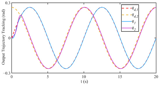
Figure 2.
The tracking results of joint angle.
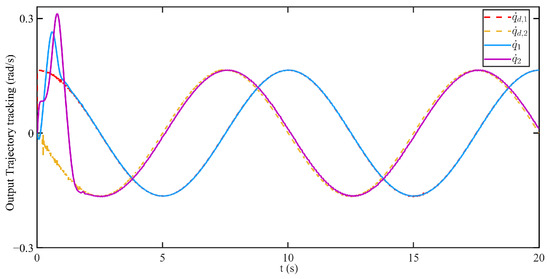
Figure 3.
The tracking results of joint velocity.
The tracking performance bounds and the tracking errors , are shown in Figure 4; the tracking performance bounds and the medial tracking errors , are shown in Figure 5.
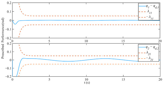
Figure 4.
Results of joint angle tracking error conforming to prescribed performance.
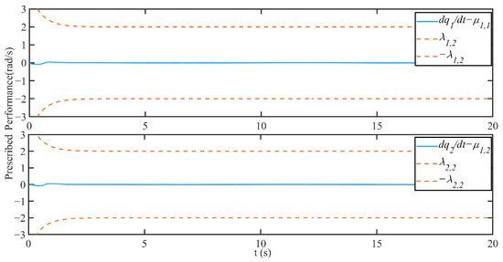
Figure 5.
Results of joint velocity tracking error conforming to prescribed performance.
As depicted in the figure, the controller achieves an excellent tracking performance, ensuring that the tracking errors are strictly confined within the prescribed performance bounds. Subsequently, Figure 6 illustrates the effect of Prescribed Performance Control when the minimum convergence rate and the maximum steady-state error are increased. Case a: ; case b: . As shown in the figure, the error still satisfies the prescribed performance requirements.
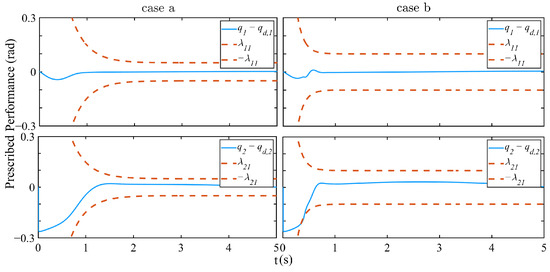
Figure 6.
Tracking error under different prescribed performances.
Figure 7 illustrates the input torque errors for the four time delays listed in Table 1, with the no delay case serving as the baseline. To demonstrate the robustness of the proposed controller against noise, some random noises are added to system (1). The tracking results of joint angle under different noise levels are presented in Figure 8.
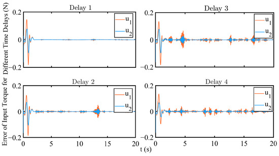
Figure 7.
The error of input torque from the no delay case under different time delays.
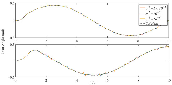
Figure 8.
The tracking results under different noise levels.
To validate its effectiveness, the performance of the proposed PPC method is benchmarked against that of Bechlious’s PPC method [34]. The comparison is presented in Figure 9. Based on the results, it can be observed that both methods demonstrate a satisfactory tracking performance in the absence of time delays. When both the control input delay and state measurement delay are fixed, Bechlious’s PPC method exhibits a slightly inferior tracking performance compared with our proposed PPC method. In scenarios with time-varying delays affecting both control input and state measurements, Bechlious’s PPC method fails to maintain stability, whereas our proposed predictive control method maintains a superior tracking performance. This demonstrates the robustness of our PPC control method across diverse delay conditions.
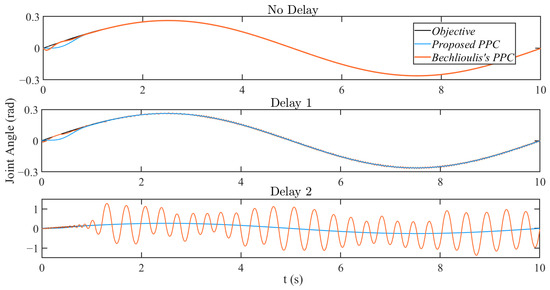
Figure 9.
Comparison result of the controller’s tracking performance under different delays.
To evaluate the disturbance observer, the following gains were selected: , and . The estimation performance of the observer against the disturbance signals and is presented in Figure 10.
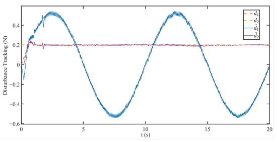
Figure 10.
Estimation error of the disturbance observer.
To validate its effectiveness, the performance of the proposed disturbance observer is benchmarked against that of Chen’s disturbance observer [35], a method widely employed in nonlinear systems. The comparative analysis is conducted under the following disturbance signals: and . The results demonstrate that the estimation error of the proposed observer converges rapidly to a small neighborhood of zero. This indicates a significantly superior estimation performance compared with Chen’s disturbance observer. A detailed comparison of the estimation errors for the disturbances and is presented in Figure 11 and Figure 12, respectively.
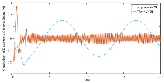
Figure 11.
Comparison result of the disturbance observer error for .
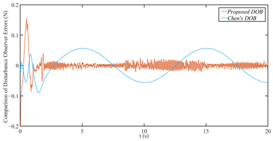
Figure 12.
Comparison result of the disturbance observer error for .
Finally, we calculated the root mean square error of the controller and the disturbance observer. The root mean square error values of the tracking effect of the controller and the root mean square error values of the disturbance observer regarding the disturbance influence are shown in Table 2.
Table 2.
Comparison of root mean square error.
The initial selection of the controller gains are , , , and . The set noise has a variance of and a mean of 0. In Table 3, the RMSE for the tracking effect of joint 1 is presented under the conditions of unchanged gain, 10% increase, 25% increase, 50% increase, and 100% increase. Among them, when , the system comes unstable; when , the system becomes unstable; and have a relatively small impact on noise; and when = 300, the system can still remain stable.
Table 3.
The sensitivity of the controller gains to noise.
Then we conducted an analysis of the discrete time effect of the system. A discretization sensitivity analysis was conducted by using zero-order retainers. We systematically changed the sampling period of the zero-order hold device and conducted simulations for each sampling period to observe and evaluate its potential impact on the system performance. The results show that when the steady-state error of the performance function is 0.1, the sampling period reaches and exceeds 0.008 s, and the system exhibits continuous and increasingly amplified oscillations, eventually leading to system instability.
4. Discussion
This paper presents a low-complexity Prescribed Performance Control (PPC) scheme for robotic systems, which guarantees that the output tracking error adheres to predefined performance bounds—namely, maximum steady-state error and minimum convergence rate—even in the presence of time delays. The controller is specifically designed to handle a known state measurement delay and an unknown but bounded control input delay. To enhance the robustness against external disturbances inherent in practical applications, a sliding-mode disturbance observer is integrated into the control framework. The simulation results on a two-degree-of-freedom (2-DOF) robotic manipulator validate the efficacy of the proposed composite control strategy, demonstrating its effectiveness under the combined challenges of state measurement and control input delays. The main limitation is that the delay cannot be too large. In the future, we will continue to study this issue and we will make conducting physical verification our top priority. Meanwhile, we will also take into account the application of large language models. For instance, reference [36] employed large language models to handle abnormal data inputs in autonomous driving. This can be applied to the processing of complex disturbances in the environment by our disturbance observer.
Author Contributions
Conceptualization, Y.W. and S.S.; methodology, Y.W. and S.S.; software, Y.W.; validation, Y.W., S.S., C.L., and W.Z.; formal analysis, Y.W.; investigation, Y.W.; resources, Y.W.; data curation, Y.W.; writing—original draft preparation, Y.W.; writing—review and editing, Y.W.; visualization, Y.W.; supervision, S.S.; project administration, Y.W. All authors have read and agreed to the published version of the manuscript.
Funding
This work was supported in part by the National Natural Science Foundation of China under Grant No. 62303074, and the Changzhou Sci&Tech Program under Grant No. CJ20235021.
Data Availability Statement
Data are contained within the article.
Conflicts of Interest
The authors declare no conflicts of interest.
Abbreviations
The following abbreviations are used in this manuscript:
| PPC | Prescribed Performance Control |
| DOF | Degree of Freedom |
| DOB | Disturbance Observer |
| RMSE | Root Mean Square Error |
References
- Darvish, K.; Penco, L.; Ramos, J.; Cisneros, R.; Pratt, J.; Yoshida, E.; Ivaldi, S.; Pucci, D. Teleoperation of humanoid robots: A survey. IEEE Trans. Robot. 2023, 39, 1706–1727. [Google Scholar] [CrossRef]
- Bekiaris-Liberis, N.; Krstic, M. Compensation of state-dependent input delay for nonlinear systems. IEEE Trans. Autom. Control 2013, 58, 275–289. [Google Scholar] [CrossRef]
- Polyakov, A.; Efimov, D.; Perruquetti, W.; Richard, J.-P. Output stabilization of time-varying input delay systems using interval observation technique. Automatica 2013, 49, 3402–3410. [Google Scholar] [CrossRef]
- Cai, X.; Bekiaris-Liberis, N.; Krstic, M. Input-to-state stability and inverse optimality of predictor feedback for multi-input linear systems. Automatica 2019, 103, 549–557. [Google Scholar] [CrossRef]
- Ran, M.; Wang, Q.; Dong, C.; Xie, L. Active disturbance rejection control for uncertain time-delay nonlinear systems. Automatica 2020, 112, 108692. [Google Scholar] [CrossRef]
- Zahaf, A.; Bououden, S.; Chadli, M.; Chemachema, M. Robust fault tolerant optimal predictive control of hybrid actuators with time-varying delay for industrial robot arm. Asian J. Control 2022, 24, 1–15. [Google Scholar] [CrossRef]
- Cao, L.; Pan, Y.; Liang, H.; Huang, T. Observer-based dynamic event-triggered control for multiagent systems with time-varying delay. IEEE Trans. Cybern. 2022, 53, 3376–3387. [Google Scholar] [CrossRef]
- Wang, J.; Wu, Y.; Chen, C.P.; Liu, Z.; Wu, W. Adaptive pi event-triggered control for mimo nonlinear systems with input delay. Inf. Sci. 2024, 677, 120817. [Google Scholar] [CrossRef]
- Cai, J.; Guo, D.; Wang, W. Adaptive fault-tolerant control of uncertain systems with unknown actuator failures and input delay. Meas. Control 2025, 58, 923–934. [Google Scholar] [CrossRef]
- Xia, X.; Pan, J.; Zhang, T.; Fang, Y. Command filter based adaptive dsc of uncertain stochastic nonlinear systems with input delay and state constraints. J. Frankl. Inst. 2022, 359, 9492–9521. [Google Scholar] [CrossRef]
- Qi, X.; Xu, S.; Liu, W. Fixed-time neural adaptive control for nonlinear asymmetric constrained systems subject to time-varying input delay. IEEE Trans. Cybern. 2025, 55, 4583–4595. [Google Scholar] [CrossRef]
- Sanz, R.; Garcia, P.; Krstic, M. Observation and stabilization of ltv systems with time-varying measurement delay. Automatica 2019, 103, 573–579. [Google Scholar] [CrossRef]
- Ferdinando, M.D.; Gennaro, S.D.; Borri, A.; Pola, G.; Pepe, P. On the robustification of digital event-based stabilizers for nonlinear time-delay systems. Nonlinear Anal. Hybrid Syst. 2024, 52, 101463. [Google Scholar] [CrossRef]
- Bikas, L.N.; Rovithakis, G.A. Prescribed performance tracking of uncertain mimo nonlinear systems in the presence of delays. IEEE Trans. Autom. Control 2021, 68, 96–107. [Google Scholar] [CrossRef]
- Weston, J.; Malisoff, M. Sequential predictors under time-varying feedback and measurement delays and sampling. IEEE Trans. Autom. Control 2018, 64, 2991–2996. [Google Scholar] [CrossRef]
- Mofid, O.; Mobayen, S.; Zhang, C.; Esakki, B. Desired tracking of delayed quadrotor uav under model uncertainty and wind disturbance using adaptive super-twisting terminal sliding mode control. ISA Trans. 2022, 123, 455–471. [Google Scholar] [CrossRef]
- Nozari, E.; Tallapragada, P.; Cortés, J. Event-triggered stabilization of nonlinear systems with time-varying sensing and actuation delay. Automatica 2020, 113, 108754. [Google Scholar] [CrossRef]
- Sun, X.-M.; Liu, K.-Z.; Wen, C.; Wang, W. Predictive control of nonlinear continuous networked control systems with large time-varying transmission delays and transmission protocols. Automatica 2016, 64, 76–85. [Google Scholar] [CrossRef]
- Bu, X. Prescribed performance control approaches, applications and challenges: A comprehensive survey. Asian J. Control 2023, 25, 241–261. [Google Scholar] [CrossRef]
- Bu, X.; Jiang, B.; Lei, H. Nonfragile quantitative prescribed performance control of waverider vehicles with actuator saturation. IEEE Trans. Aerosp. Electron. Syst. 2022, 58, 3538–3548. [Google Scholar] [CrossRef]
- Ficuciello, F.; Villani, L.; Siciliano, B. Variable impedance control of redundant manipulators for intuitive human–robot physical interaction. IEEE Trans. Robot. 2015, 31, 850–863. [Google Scholar] [CrossRef]
- Chen, W.-H.; Ballance, D.J.; Gawthrop, P.J.; O’Reilly, J. A nonlinear disturbance observer for robotic manipulators. IEEE Trans. Ind. Electron. 2000, 47, 932–938. [Google Scholar] [CrossRef]
- Guo, K.; Shi, P.; Wang, P.; He, C.; Zhang, H. Non-singular terminal sliding mode controller with nonlinear disturbance observer for robotic manipulator. Electronics 2023, 12, 849. [Google Scholar] [CrossRef]
- Farhat, M.; Kali, Y.; Saad, M.; Rahman, M.H.; Lopez-Herrejon, R.E. Walking position commanded nao robot using nonlinear disturbance observer-based fixed-time terminal sliding mode. ISA Trans. 2024, 146, 592–602. [Google Scholar] [CrossRef] [PubMed]
- Liu, L.; Yue, X.; Wen, H.; Hao, Z.; Zhu, Y. A globally exponentially stable observer for torque estimation with only position measurement. Proc. Inst. Mech. Eng. Part I J. Syst. Control Eng. 2024, 238, 238–251. [Google Scholar] [CrossRef]
- Junplod, G.; Kornmaneesang, W.; Chen, S.-L.; Wongsa, S. Modeling of an external force estimator for an end-effector of a robot by neural networks. J. Chin. Inst. Eng. 2023, 46, 895–904. [Google Scholar] [CrossRef]
- Su, H.; Qi, W.; Li, Z.; Chen, Z.; Ferrigno, G.; Momi, E.D. Deep neural network approach in emg-based force estimation for human–robot interaction. IEEE Trans. Artif. Intell. 2021, 2, 404–412. [Google Scholar] [CrossRef]
- Zhao, H.; Guo, Y.; Liu, Y.; Jin, J. Multirobot unknown environment exploration and obstacle avoidance based on a voronoi diagram and reinforcement learning. Expert Syst. Appl. 2025, 264, 125900. [Google Scholar] [CrossRef]
- Bechlioulis, C.P.; Rovithakis, G.A. Robust adaptive control of feedback linearizable mimo nonlinear systems with prescribed performance. IEEE Trans. Autom. Control 2008, 53, 2090–2099. [Google Scholar] [CrossRef]
- Sun, T.; Cheng, L.; Wang, W.; Pan, Y. Semiglobal exponential control of euler–lagrange systems using a sliding-mode disturbance observer. Automatica 2020, 112, 108677. [Google Scholar] [CrossRef]
- Bikas, L.N.; Sidiropoulos, A.; Rovithakis, G.A.; Doulgeri, Z. Model-free control of bilateral robotic teleoperation with delays and prescribed performance guarantees. IFAC Pap. 2023, 56, 9972–9977. [Google Scholar] [CrossRef]
- Li, Z.; Zhai, J. Super-twisting sliding mode trajectory tracking adaptive control of wheeled mobile robots with disturbance observer. Int. J. Robust Nonlinear Control 2022, 32, 9869–9881. [Google Scholar] [CrossRef]
- Moreno, J.A.; Osorio, M. A lyapunov approach to second-order sliding mode controllers and observers. In Proceedings of the 2008 47th IEEE Conference on Decision and Control, Cancun, Mexico, 9–11 December 2008; pp. 2856–2861. [Google Scholar]
- Bechlioulis, C.P.; Rovithakis, G.A. A low-complexity global approximation-free control scheme with prescribed performance for unknown pure feedback systems. Automatica 2014, 50, 1217–1226. [Google Scholar] [CrossRef]
- Chen, W.-H. Disturbance observer based control for nonlinear systems. IEEE/ASME Trans. Mechatron. 2004, 9, 706–710. [Google Scholar] [CrossRef]
- Zou, Y.; Xu, Z.; Zhang, Q.; Lin, Z.; Wang, T.; Liu, Z.; Li, D. Few-shot learning with manifold-enhanced llm for handling anomalous perception inputs in autonomous driving. IEEE Trans. Intell. Transp. Syst. 2025. [Google Scholar] [CrossRef]


Disclaimer/Publisher’s Note: The statements, opinions and data contained in all publications are solely those of the individual author(s) and contributor(s) and not of MDPI and/or the editor(s). MDPI and/or the editor(s) disclaim responsibility for any injury to people or property resulting from any ideas, methods, instructions or products referred to in the content. |
© 2025 by the authors. Licensee MDPI, Basel, Switzerland. This article is an open access article distributed under the terms and conditions of the Creative Commons Attribution (CC BY) license (https://creativecommons.org/licenses/by/4.0/).