Article

ADEmono-SLAM: Absolute Depth Estimation for Monocular Visual Simultaneous Localization and Mapping in Complex Environments

1
School of Intelligent Engineering and Intelligent Manufacturing, Hunan University of Technology and Business, Changsha 410205, China
2
Xiangjiang Laboratory, Changsha 410205, China
*
Authors to whom correspondence should be addressed.
Electronics 2025, 14(20), 4126; https://doi.org/10.3390/electronics14204126
Submission received: 3 October 2025 / Revised: 12 October 2025 / Accepted: 15 October 2025 / Published: 21 October 2025
(This article belongs to the Special Issue Digital Intelligence Technology and Applications, 2nd Edition)

Abstract

Aiming to address the problems of scale uncertainty and dynamic object interference in monocular visual simultaneous localization and mapping (SLAM), this paper proposes an absolute depth estimation network-based monocular visual SLAM method, namely, ADEmono-SLAM. Firstly, some detail features including oriented fast and rotated brief (ORB) features of input image are extracted. An object depth map is obtained through an absolute depth estimation network, and some reliable feature points are obtained by a dynamic interference filtering algorithm. Through these operations, the potential dynamic interference points are eliminated. Secondly, the absolute depth image is obtained by using the monocular depth estimation network, in which a dynamic point elimination algorithm using target detection is designed to eliminate dynamic interference points. Finally, the camera poses and map information are obtained by static feature point matching optimization. Thus, the remote points are randomly filtered by combining the depth values of the feature points. Experiments on the karlsruhe institute of technology and toyota technological institute (KITTI) dataset, technical university of munich (TUM) dataset, and mobile robot platform show that the proposed method can obtain sparse maps with absolute scale and improve the pose estimation accuracy of monocular SLAM in various scenarios. Compared with existing methods, the maximum error is reduced by about 80%, which provides an effective method or idea for the application of monocular SLAM in the complex environment.

1. Introduction

Simultaneous localization and mapping (SLAM) has been a core research topic in robotics in recent years [1,2]. It aims to enable robots to estimate their motion and simultaneously construct a map of unknown environments. SLAM maps are typically categorized as sparse, semi-dense, or dense, depending on the density of reconstructed features. Sensors used in SLAM include LiDAR, cameras, and odometers. Cameras can not only provide rich environmental information, but also offer low cost, light weight, and compact size [3,4]. Visual SLAM relying on cameras as the primary sensor has gained popularity. Consequently, visual SLAM has been widely applied in autonomous driving, service robots, and AR/VR.
According to sensing modality, camera types can be divided into monocular, stereo, and red green blue-depth (RGB-D) [5]. Monocular SLAM with only one camera achieves the lowest cost, but suffers from the following three inherent scientific challenges [6,7,8]. (1) There is scale unobservability. Based on the pinhole projection model, a 2D pixel coordinate ( u ,   v ) corresponds to infinitely many 3D points along the optical ray. The depth Z cannot be uniquely determined, resulting in scale ambiguity. Even after initialization, the relative scale drifts during long-distance motion due to the lack of metric constraints. (2) There is some dynamic interference. In real-world scenes, moving objects (e.g., pedestrians, vehicles) violate the static scene assumption. Their feature points introduce inconsistent motion cues, which cause errors in motion estimation and data association. (3) There are distant feature noises. Feature points with large depth values contribute weak geometric constraints, while their depth estimation errors increase nonlinearly with distance. Feature points may introduce noise, but removing them entirely may result in insufficient effective features.
Traditional geometric methods including PTAM [9], ORB-SLAM [10,11,12], and direct sparse odometry (DSO) [13] treat above issues as engineering problems to be alleviated, often by incorporating additional sensors such as inertial measurement units (IMUs). Unfortunately, such solutions increase system complexity and still fail to resolve the fundamental scientific limitations of monocular vision. In recent years, deep-learning-integrated approaches have made great progress [14,15]. Some end-to-end visual odometry (VO) models such as DeepVO [16] and ESP-VO [17] learn motion patterns from large-scale data. However, the scale estimation lacks explicit metric constraints and generalizes poorly across domains [18,19,20,21,22]. Hybrid methods combining semantic cues with geometry improve robustness in dynamic scenes [23]. Hybrid methods lack a principled integration of semantic and geometric information, leading to unstable performance. Obviously, it is of great significance to develop monocular SLAM frameworks that fundamentally resolve scale ambiguity, dynamic interference, and distant feature noise using only visual information.
This paper proposes ADEmono-SLAM, a monocular SLAM system that integrates absolute depth estimation into the traditional framework. The main contributions are summarized as follows. (1) We propose an ADEmono-SLAM approach based on the absolute depth estimation network. By incorporating metric depth produced from the absolute depth estimation network, ADEmono-SLAM is able to resolve the inherent scale ambiguity of monocular vision and significantly reduces scale drift in long distance motion. (2) A dynamic interference suppression approach is built for feature point detection. A fusion mechanism including semantic and geometric is built to remove dynamic feature points, which can improve robustness in dynamic environments. (3) A probabilistic distant feature filtering algorithm is proposed. A noise-aware strategy selectively filters long-distance points, balancing noise suppression and feature completeness. (4) Some comprehensive validations are performed on some datasets and a mobile robot platform. Experiments on public datasets and the mobile robot platform demonstrate that ADEmono-SLAM achieves superior accuracy and robustness compared with state-of-the-art monocular SLAM and popular VO methods.

2. Related Work

In this section, we review the existing methods from the perspective of how they address the core scientific challenges of monocular SLAM: scale unobservability, dynamic interference, and distant feature noise.

2.1. SLAM Based on Traditional Geometric Methods

Traditional geometric methods form the foundation of visual SLAM. With these methods, one can mitigate scale ambiguity and motion estimation errors. Davison proposed the first real-time monocular SLAM system based on extended kalman filter (EKF), laying the groundwork for monocular motion estimation [8]. However, this method could not resolve the inherent scale unobservability of monocular vision, leading to uncontrolled drift in large-scale scenes. Klein introduced parallel tracking and mapping (PTAM), which separated tracking and mapping into parallel threads, establishing the classic front-end/back-end framework [9]. While PTAM improved real-time performance, it still relied on relative depth from stereo initialization, failing to address the scientific root of scale ambiguity: the lack of metric constraints in monocular projection. Further, Mur-Artal developed the ORB-SLAM series methods integrating IMU to alleviate scale drift [10,11]. However, these approaches do not fundamentally solve scale unobservability. Instead, they transfer the problem to IMU calibration and noise accumulation, which will lead to renewed drift when IMU data degrades.
For dynamic scenes, ORB-SLAM3 relies on geometric consistency checks, which suffer from high false-positive rates in low-texture regions where dynamic and static features are indistinguishable [12]. Moreover, Engel proposed a direct method that minimizes image brightness errors [13]. While avoiding feature extraction instability, the direct method still faces scale ambiguity in monocular mode and lacks targeted handling of distant features, where photometric errors accumulate due to low resolution and noise. In summary, traditional geometric methods treat scale ambiguity as an engineering problem to be mitigated via IMU fusion, and their handling of dynamic and distant features remains empirically driven.

2.2. SLAM Based on Deep Learning Methods

In recent years, deep learning methods have been widely applied in various fields [14]. Beyond geometry-only pipelines, a broader perspective on SLAM with deep learning has identified open challenges in scale recovery and dynamic scenes, which can provide a taxonomy and research roadmap for learning-augmented localization and mapping [15]. Such design principles, though developed for service recommendation, offer insights into balancing real-time performance and data security in SLAM deployment. Deep learning has introduced new tools for addressing SLAM’s scientific challenges, but existing methods still have limitations in tackling scale unobservability, dynamic interference, and distant feature noise.
Among deep learning-based methods, end-to-end methods use recurrent convolutional networks to learn motion patterns from data [16,17]. DeepVO outperforms traditional vision odometers in some scenarios [16]. The scale estimation relies on implicit data-driven patterns rather than explicit metric constraints, leading to poor generalization across domains. Additionally, UndeepVO is able to recover absolute scale using spatial-temporal loss [18]. The absolute scale is derived from relative depth transformation, which lacks strict metric consistency and results in cumulative errors in large-scale scenes.
Recently, some methods combining geometry and deep learning have shown more promise for addressing core scientific issues [19]. For instance, RAUM-VO is able to adjust rotation via epipolar constraints and uses deep networks for keypoint matching [20]. This method improves pose accuracy but relies on relative depth, leaving scale ambiguity unresolved in long-distance motion. In addition, TSformer-VO uses transformers for feature extraction [21]. However, the handling of distant features has no targeted noise filtering, and leads to performance degradation in large-scale outdoor scenes. Further, Zhu proposed DeepAVO, which uses attention modules to refine pose estimates [22]. While enhancing feature discriminability, it does not address the fundamental scale unobservability of monocular vision, so application in metric-required scenarios is limited. Ma proposed the DSOD method that integrates semantic segmentation with DSO to handle dynamic scenes [23]. While effective in some cases, DSOD does not establish a statistical relationship between semantic labels and geometric motion consistency, leading to the over-filtering of static features in semantically ambiguous regions such as stationary vehicles misclassified as dynamic.
Basically, existing methods have three key shortcomings. Traditional methods avoid rather than solve scale unobservability, while deep learning methods lack explicit metric constraints, leading to unstable scale in large scenes. Moreover, geometric methods rely on fragile consistency checks, while semantic methods lack a principled integration of semantic and geometric cues, leading to either under- or over-filtering. No existing method explicitly models the nonlinear growth of depth error with distance, resulting in either excessive noise from retained distant features or insufficient features from aggressive filtering.
The key challenges of monocular SLAM originate from the inherent limitations of single-camera vision in recovering 3D information. These limitations manifest as scale ambiguity, dynamic interference, and distant feature noise. In monocular SLAM, the projection from 3D world coordinates to 2D image coordinates is modeled by the pinhole camera model [5]. The depth cannot be uniquely determined from a single 2D observation. All feature points along the ray through the camera center and pixel correspond to the same projection. This leads to scale unobservability, which lacks an absolute metric reference.
Besides that, dynamic objects violate the static scene assumption of SLAM. Their feature displacements between frames contain both camera motion and object self-motion, resulting in incorrect pose estimation when using purely geometric constraints. Traditional random sample consensus (RANSAC)-based outlier rejection fails in low-texture regions, while semantic segmentation-based approaches often over-filter static objects misclassified as dynamic. Therefore, a more reliable semantic and geometric fusion strategy is needed to identify and remove dynamic features while preserving valid static ones.
Feature points at large depth values contribute little to pose estimation, since their parallax is minimal across adjacent frames. At the same time, their depth estimation error grows nonlinearly with distance due to limited image resolution and sensitivity to atmospheric scattering and sensor noise. Retaining such features introduces uncertainty, while discarding all of them may cause insufficient constraints in texture-poor regions. Existing methods typically apply empirical thresholds, without modeling the statistical distribution of depth errors. This motivates a probabilistic filtering strategy that reduces noise while maintaining feature completeness.
To fundamentally address these challenges, we propose an integrated ADEmono-SLAM framework in this paper. In the framework, an absolute depth estimation network is proposed by providing metric constraints to eliminate scale ambiguity. Further, we build a semantic and geometric fusion method, which is able to statistically model dynamic interference through target detection and feature filtering. Additionally, a probabilistic distant feature filtering approach is proposed through leveraging noise distribution characteristics to balance noise suppression and feature completeness.

3. The Proposed Method

To address the challenges of monocular SLAM including scale ambiguity, dynamic interference, and distant feature noise, this paper proposes ADEmono-SLAM. The overall system is illustrated in Figure 1. The ADEmono-SLAM framework integrates absolute depth estimation with geometric constraints. Input images are processed in parallel through three procedures: objection detection, absolute depth estimation, and ORB feature point extraction. The feature points and their depth values produced by absolute depth estimation and ORB feature point extraction are used as input for the long-distance point-filtering module. Some interference points are removed by long-distance feature filtering. Moreover, objection detection is tackled by the YOLOv5 network. After dynamic feature removal, the outputs are fused for feature matching and pose optimization to obtain camera poses and map points. For each input frame, ORB features and binary descriptors are extracted. A monocular absolute depth estimator produces a depth map that supplies scale and distance cues. Depth information is used to randomly filter distant or unreliable features. Further, an object detection module identifies potentially dynamic objects so that feature points on moving targets can be excluded. The remaining stable features are matched and refined via nonlinear optimization to jointly optimize the camera trajectory and map points.

3.1. Absolute Depth Estimation Network

The inability to recover absolute depth from 2D projections causes the fundamental problem of scale ambiguity in monocular SLAM. To resolve this, an absolute depth estimation network based on ZoeDepth [24] is built to provide metric depth for feature points and converts the infinite solutions of monocular projection into unique metric solutions. The overall architecture of the absolute depth estimation network is shown in Figure 2. By providing absolute depth for feature points, ADEmono-SLAM resolves the inherent scale ambiguity and ensures metrically consistent pose estimation.
For a 3D point ( X ,   Y ,   Z ) in the camera frame, its projection ( u ,   v ) onto the image plane is given by following equation.
u v 1 = 1 Z · f x 0 c x 0 f y c y 0 0 1 · X Y Z  
where f x ,   f y are focal lengths, and c x ,   c y is the principal point.
The absolute depth estimation network is designed in two stages, following the staged optimization principle and supported by stability analyses of neural networks, including those on fuzzy logic-based aggregation operators. These analyses, though focused on decision-making, highlight the importance of robust feature fusion to meet a core requirement for stable depth estimation in the absolute depth estimation network.
The primary idea of absolute depth estimation network remains two complementary perspectives. Firstly, hybrid feature fusion incorporating relative depth prediction is performed by federated learning for robust decision-making [25,26]. On this basis, an absolute depth estimation network is built to combine hierarchical visual features to broaden depth prediction generalization. At this point, we employ decision making technology to enhance the depth prediction [27]. Secondly, hierarchical relation learning strategies are employed to combine compressive sensing networks that optimize data transmission via layered feature correlations [28]. The absolute depth estimation network’s encoder–decoder structure leverages these hierarchical dependencies to capture multi-scale depth relationships. This dual-inspiration framework balances cross-modal feature synergy and structural depth learning, aligning with cutting-edge multi-source optimization paradigms [29,30,31]. The encoder–decoder backbone is implemented using PyTorch 1.10.1 Image Models [32]. The second stage refines depth using a metric bin module inspired using LocalBins [33].
In the absolute depth estimation network, pixel-wise depth prediction aligns with point-by-point feature extraction methods [34]. Fine-grained feature analysis, similar to depth map generation, is able to improve task-specific accuracy. Inspired by LocalBins [33] and existing encoder–decoder architecture, we do not estimate the global distribution of depth values for the input image while predicting the depth distribution within a local range for each pixel. One can predict not only the output of the last layer of the decoder, but also combine all layers of the decoder to predict the bin centers for each pixel. The final depth value of a pixel is obtained by summing the linear products of the center values of the bins and their predicted probabilities. In the bottleneck layer, each pixel predicts Ns different seed bins and then uses a classifier multi-layer perceptron (MLP) to split each bin in two. After each layer of the decoder, the number of bin centers doubles. For instance, at the n-th decoder layer, each pixel will have 2nNs bins. The softmax function is used to predict the scores corresponding to each bin center, and the final depth of pixel i can be obtained using Equation (2).
  Z i = k = 1 N sum P i k · C i k  
where   N sum   =   2 n · N s .  Nsum represents the number of sub-bins at a certain layer of the decoder, P represents the softmax function prediction score for a certain pixel point, C represents the corresponding center value of the sub-bin for a certain pixel point, and Zi represents the final depth value of the i-th pixel point.
Due to the order of the bins themselves, the softmax method may result in significant differences in probability values for similar pixels. To improve probability prediction, we replace softmax with a log-binomial distribution shown in Equations (3) and (4). This improvement can effectively align with hybrid feature processing, and multi-level fusion strengthens fine-grained estimation. It is reasonable that sequence modeling for the vision odometer leverages long-term temporal consistency from sequential data to stabilize predictions [35]. The log-binomial distribution embeds implicit temporal priors such as depth continuity to mitigate frame-wise noise. In addition, the probabilistic depth calculation similarly enhances robustness under distribution shifts by explicitly modeling uncertainty.
P i ; N sum , q = N sum i · q i · 1 q N sum i
P i = softmax log ( p i ) t N sum i = 1
Among them, p i   =   P i ; N sum , q , which represents the calculation of the binomial distribution value for the i-th warehouse center. q and t are predicted based on the decoder features, representing the mode and temperature, respectively. To obtain the normalized probability, the softmax function is still used. Then, the t-temperature is applied to control the final distribution. P(i) indicates the final probability value of the z-th binary center, and the final absolute depth value of the pixel is updated according to Equation (2).
It is crucial to tackle sequential tasks for visual SLAM due to the temporal consistency problem [19]. Absolute depth estimation network training is solely based on single images, aiming for metric-scale accuracy and zero-shot transfer. Its training includes relative depth pre-training and metric depth fine-tuning but lacks consistency constraints on sequential images. As single image depth estimation learns the depth based on stereo image pairs, it does not suffer from the scale issue. To tackle this problem, a global absolute scale extracting method is employed during absolute depth estimation network training [15]. Suppose that the estimated depth value in pixels from single-image depth estimation is z s i , j , and the estimated depth value in the same point from the absolute depth estimation network is z ade i , j . The global scale factor can be computed as
S g l o b a l   = i = 0 m j = 0 n z s i , j z ade i , j m × n
where m and n are the dimension of image I(i,j).
As the absolute depth estimation network estimates depth based on image sequences, the predicted depth map would be more accurately estimated once the scale is corrected. Similar to the VO method [15], we also optimize the single image depth estimation by minimizing the depth difference between z ade i , j and single image depth estimation S g l o b a l × z ade i , j z s i , j . A global consistency loss function is built to enforce the predicted depth maps from single image estimation be similar to that from the absolute depth estimation network. By exploiting temporal sequence and spatial image pair simultaneously, their performance can mutually improve compared with predicting either of them independently. The global consistency loss is defined as follows:
L g l o b a l   =   i = 0 m j = 0 n D t s i , j D t a d e i , j × S g l o b a l  
where D t s i , j is the estimated depth map from the single image at time t. D t a d e i , j is the estimated depth map from absolute depth estimation network for the same input image. S g l o b a l is the global scale factor.

3.2. Dynamic Interference Point Removal

Moving objects such as pedestrians and bicycles violate the static scene assumption and introduce inconsistent motion cues [36]. To deal with this problem, we address the issue of excluding interference from potential dynamic objects in images by designing a dynamic interference point removal algorithm based on rapid object detection. It identifies interference feature points among potential dynamic objects that are actually in motion, thereby preventing these interference points from being included in subsequent matching and optimization processes, and enhancing the system’s resilience to interference.
In order to extract ORB feature points from the input image, we employ a YOLOv5 network [37] as a fast object detection model to detect in real time whether there are any of the priori objects while obtaining feature points. We train YOLOv5 network using a public image database that includes some partially occluded objects such as people, bicycles, cars, motorcycles, buses, and trucks. The network is similar to other popular convolutional neural network structures [38,39,40,41,42]. The ORB feature point extraction process is denoted by the following equation:
O i   =   F I i
To further reduce the deviation between the depth values predicted by the depth estimation network and their actual distances in different real-world scenarios, we designed a feature point enhancement algorithm. Assuming the image after extracting ORB feature points is R, with a width of w and a height of h, the set of feature points is O i i = 1 ,   2 ,   3 N , where N is the total number of feature points extracted from the current image. The depth image obtained from the depth estimation network is D, and the depth corresponding to each feature point is D i i = 1 ,   2 ,   3 N . Then, the image R is divided into equal-area segments similar to a quadtree structure, resulting in four equal-area image blocks after one division that is described as follows:
R i = R 0       0 x < w / 2   and   0 y < h / 2 R 1       w / 2 x < w   a n d   0 y < h / 2 R 2       w / 2 x < w   a n d   h / 2 y < h R 3       0 x < w / 2   a n d   h / 2 y < h    
where Ri represents four equal-area blocks; sequentially in the order of subscript: top left; top right; bottom right; and bottom left image blocks. x and y are the coordinate values of the pixel width and height, respectively.
After the initial partitioning, each sub-block undergoes uniform processing. For the top left image block R0, the subset of feature points is O 0 _ i i = 1 ,   2 ,   3 N 0 , where N0 is the total number of feature points in that block, and the depth values of each feature point are D 0 _ i i = 1 ,   2 ,   3 N 0 . Additionally, specific weights are assigned to each feature point based on its depth value and the Euclidean distance between pixel coordinates, with the weight defined as the edge length between two points, denoted as W 0 _ i . Equation (9) describes how to calculate the weight value.
  W 0 _ i = M 0 x 1 M 0 x 2 2 × P % exp D 0 i M i n / M a x M i n × Q %
where, i = 1 , 2 , 3 N 0 . R 0 _ x 1 is the starting point of the edge, and R 0 _ x 2 is the endpoint of the edge, meaning that the above formula describes the weight value of the directed edge from the starting point to the endpoint. Max and Min represent the maximum and minimum depth values within this image block, respectively. P and Q are proportion parameters that are reasonably adjusted based on the width and height of the input image. Their values can be determined by image size.
Then, we set the feature point with the minimum depth value in the image block as the starting point, and begin searching for the next point. During the search process, the point with the maximum weight relative to the starting point is identified. The search process is repeated until the number of identified feature points reaches 3/4 × N0, at which point the search stops and the remaining 1/4 × N0 points are filtered out. After all four sub-blocks have been processed, each sub-block also undergoes the aforementioned recursive operation to further enhance the robustness and randomness of the selected point set, while ensuring the uniform distribution of the original feature points. Figure 3 describes the main process of this algorithm.
As can be seen in Figure 3, after extracting feature points from the image, the first block division is performed, followed by the elimination of some feature points. In the second recursive block division, additional feature points are also removed. This algorithm not only maintains the uniformity of the feature points after processing, but also further selects more effective feature points based on the relative error of the absolute depth values, providing a solid foundation for subsequent feature matching and pose optimization.
If target objects have appeared, a rectangle is drawn around the targets and their pixel area calculated. The size of potential dynamic targets based on the area ratio of different targets to the whole image will be then determined. Assume that the current frame with dynamic target objects is M, and set a specific target as a mask point set mask, as shown in Equation (10). Equation (11) describes the method for determining whether a pixel point is within the mask, where (Px, Py) represents the two-dimensional coordinates of the point to be evaluated, and (P1_x, P1_y) and (P2_x, P2_y) represent the two-dimensional coordinates of the top-left and bottom-right corners of the mask boundary rectangle. To avoid interference from edge pixels of dynamic targets, the mask area is expanded outward by a distance of d pixels.
  M i =   O i   Mask i O i
Mask i =   P ix , P iy   P 1 _ x d < P ix < P 2 _ x + d   and   P 1 _ y d < P iy < P 2 _ y + d }  
where d = P 2 _ y P 1 _ y 2 + P 2 _ x P 1 _ x 2 × 2 % .
Since small targets often contain few feature points, all feature points within the small target are removed. The feature points in the large target undergo a secondary determination of whether their real motion state is dynamic. Each feature point in the potential dynamic large target is processed as follows. Assume that the feature points contained are O i i = 1 ,   2 ,   3 N , the feature points in the target box are M a s k i i = 1 ,   2 ,   3 P , and the feature points in the background are B j i = 1 ,   2 ,   3 Q . After matching feature points between the current frame and the previous frame, the t static points from the current frame’s background that have the shortest Hamming distance to the previous frame’s binary descriptors are selected. The mean pixel distance difference between the points to be judged in the current target box and these t static points is calculated; feature points with a difference greater than the threshold D d i s are considered dynamic points. Equation (12) describes the set of feature points within a specific box that meet the preliminary static model.
O M i = O i   1 t × j = 1 t M a s k i B j 2 < D d i s  
where O M i M a s k i , i = 1 , 2 , 3 P .
Furthermore, in order to avoid the coincidence of moving objects moving consistently in the projection direction, for feature points O M i i = 1 ,   2 ,   3 P within the threshold D d i s range, the current frame’s pose Tc is obtained based on a constant velocity model. Using the principles of epipolar geometry, the matching points are projected onto the current image to obtain the projected points. If the pixel distance between the feature point to be judged and the projected point exceeds a specific threshold Dmin, it is also considered a dynamic point. The remaining static points are combined with the target external background points to serve as the final feature points for inter-frame matching. The set of static points within the final frame is represented as follows:
O L i = O M i     | | K     T c     P w   O M i | | 2 < D m i n ,  
where O L i O M i , i = 1 , 2 , 3 P .
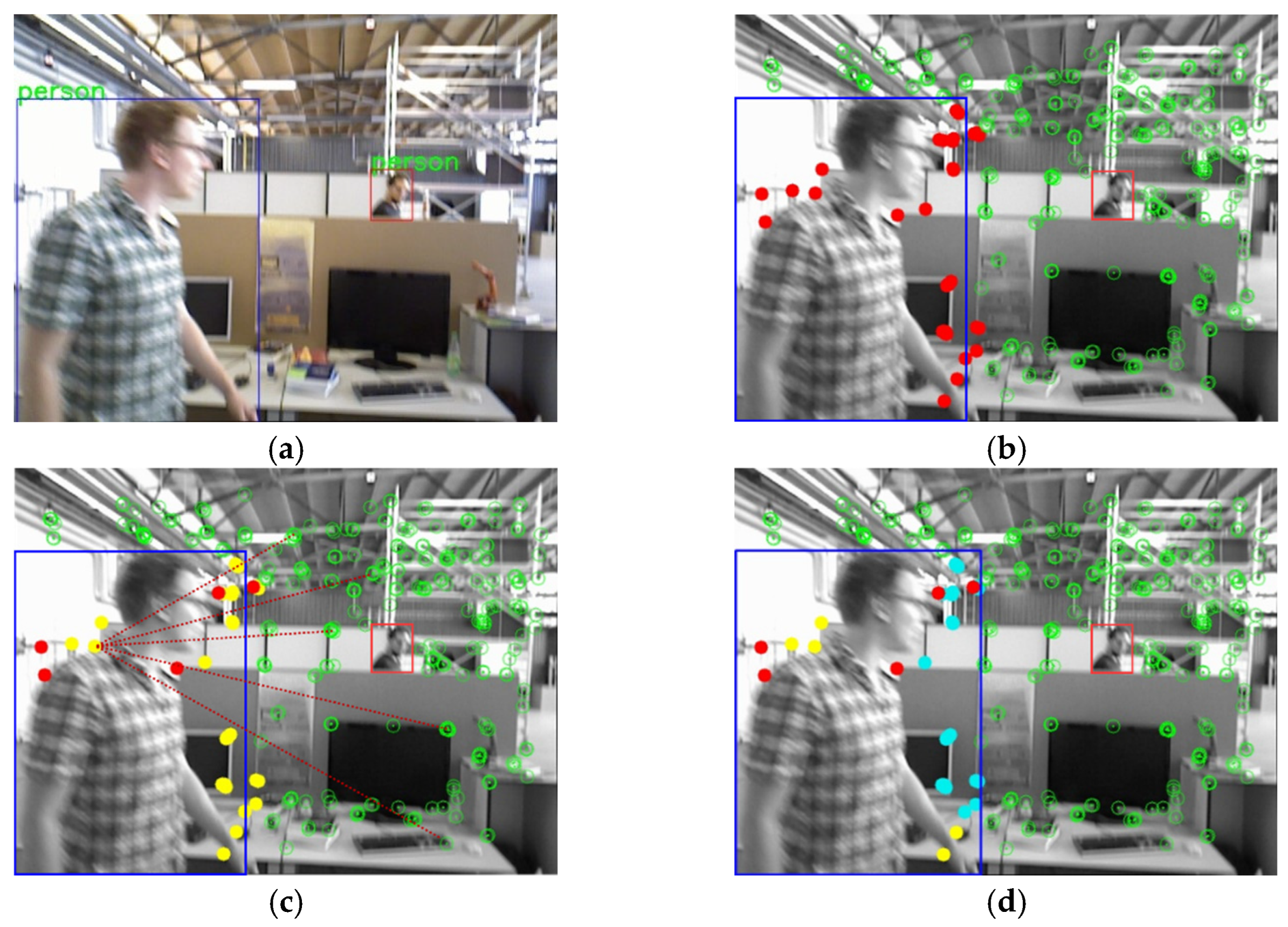
In this context, OLi represents static points within the target frame, K refers to the camera’s intrinsic parameters, and Pw corresponds to the three-dimensional coordinates in the world coordinate system of matching points from the current frame to the previous frame. Figure 4 illustrates the main process of the dynamic interference point removal algorithm. Figure 4a shows target detection and differentiation between large and small targets. Figure 4b addresses the classification processing of feature points among different targets, where the green circles represent static feature points extracted from the static background-these points are initially identified as potential reliable features before interference removal. Figure 4c displays the feature points after the first removal, colored in yellow, and Figure 4d shows the feature points after the second removal, colored in blue. Clearly, this mechanism effectively eliminates motion ambiguity caused by dynamic objects. Its design principle aligns with risk management frameworks for complex systems. Similar to how large-group failure mode analysis identifies and mitigates critical risks, the dynamic feature removal strategy isolates abnormal motion cues to preserve pose estimation stability.

3.3. Long-Distance Point Filtering

Feature points with large depth values (often greater than 30 m) provide weak geometric constraints, while their depth errors increase nonlinearly with distance. Large depth values introduce noise, and small depth values reduce feature sufficiency. To balance this trade-off, ADEmono-SLAM adopts a probabilistic filtering strategy. As the core of probabilistic filtering strategy, the long-distance point filtering module proposed in this paper, which is described in Algorithm 1 (Distant point filtering algorithm). Depth values are obtained from the absolute depth estimation network and a threshold of Zth = 30 m is applied. Then, 50% of the feature points will be randomly filtered using a time-based random seed when Z > Zth. This approach is able to significantly preserve sufficient constraints while reducing noise.
By avoiding both over-filtering and under-filtering, this strategy stabilizes pose estimation in large-scale outdoor scenes, anchored in two complementary theoretical pillars. Firstly, dynamic noise mitigation from sequence modeling can filter noisy medical data to boost diagnostic reliability [38]. The probabilistic filtering targets distant feature noise and suppresses irrelevant signals to stabilize convergence. This noise-controlled system can enhance the geometric pose estimation. Secondly, a hybrid feature prioritization from geophysical inversion can balance local–global features for resistivity inversion by prioritizing trustworthy inputs. The proposed method filters long-range points while retaining geometrically stable features. By bridging these two domains, the proposed strategy harmonizes noise resilience and feature reliability.
Algorithm 1: Distant point filtering algorithm
Input:Image to be processed M
Set Depth Threshold fd
Output:Filter to get reliable feature points for feature matching
1:All feature points KP of the monocular image M output in the previous stage
2: M predicts each pixel of the current image through the absolute depth estimation network to obtain a depth map D
3:Set a random seed with respect to time
4: for   the i feature point:
5: Calculate the corresponding depth value di according to the two-dimensional pixel coordinates of the feature point
6: if(di > fd)
7: Obtain a random number num i from 0 to 1
8: if num i   <   0.5
9: Eliminate long-distance feature points with unreliable depth values KP i
10: else ;
11: else ;
12: Return KP     KP i

4. Experiment and Analysis

In order to evaluate the performance of the proposed method, some experiments were carried out on the outdoor public dataset KITTI [6], the indoor public dataset TUM RGBD [7] and a mobile robot platform. To eliminate random errors in the system, each experiment was repeated 5 times, and the median was used as the final result. The experimental environment was as follows: an Intel Core i9-9900 CPU (Intel Corporation, Santa Clara, CA, USA) with 3.1 GHz, memory with 64 G and NVIDIA Quadro P2200 GPU (NVIDIA Corporation, Santa Clara, CA, USA). All experiments were conducted in the Ubuntu18.04 operating system (Canonical Ltd., London, UK).
To fairly compare the results of various methods, we adopted the measurement method of pose and trajectory evaluation commonly used in SLAM, which is consistent with the absolute translation root mean square error (RMSE) t a b s used in ORB-SLAM2 [11]. The calculation method of this index is shown in Equation (14).
  t a b s = 1 N · i = 1 N | | t r a n s F i   | | 1 / 2
where   F i   = T g t , i 1 · S · T e s t , i , T g t   represents the ground truth trajectory, T e s t represents the estimated trajectory, S represents the similarity transformation matrix between T g t   and T e s t , F i   represents the absolute trajectory error of step i , and t r a n s F i   represents the scalar value of the translation part in the brackets.

4.1. Experiments on KITTI Odometer Image Dataset

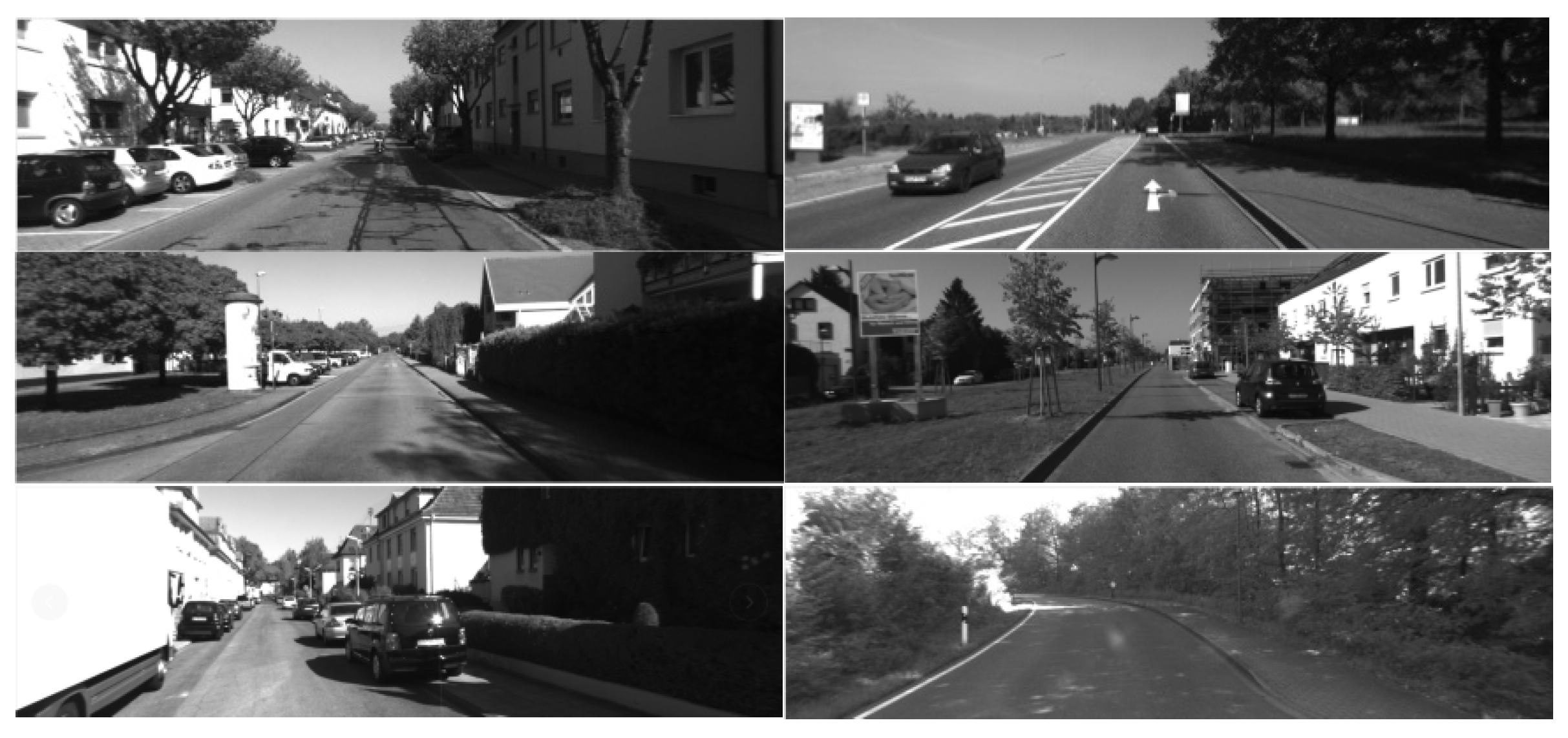
The KITTI odometer image dataset is a public outdoor dataset commonly used in the field of autonomous driving and SLAM [6]. It typically includes some cities and highway scenes in Germany. The dataset was recorded by a vehicle-mounted stereo camera with an image resolution of 1240 × 376. The odometer data of the KITTI dataset organizes images and trajectory information for different sequences. Different sequences contain different real-life scenarios. For example, the sequence 00–10 is urban, highway, urban, country, country, country, urban, urban, urban, urban, and country, respectively, as shown in Figure 5. In our experiment, nine sequences were employed, among which sequences 00, 02, 05, 06, 07, and 09 contained loop closure.
In order to measure the performance of our approach, we compared ADEmono-SLAM with some typical geometric methods including ORB-SLAM2 and ORB-SLAM3 variants. ORB-SLAM3 includes two variants: ORB-SLAM3 (short version) and ORB-SLAM3 (full version). ORB-SLAM3 (short version) does not have loop detection, while ORB-SLAM3 (full version) and ORB-SLAM2 have loop detection. ADEmono-SLAM has no loop detection. Table 1 shows the results of different methods on various sequences.
The t a b s of ADEmono-SLAM on sequences 08 and 10 are 14.51 and 4.06, respectively, which are the lowest values among these methods. The t a b s on the above two sequences was significantly reduced by 72.06% and 48.15%, respectively, compared with ORB-SLAM3 (short version). On sequences 02, 05, and 06, the t a b s of ADEmono-SLAM are 22.99, 5.18, and 4.33, respectively, which are also the best results among these methods. Specifically, the t a b s of ADEmono-SLAM reduced by 16.30%, 1.70%, and 71.23% compared with ORB-SLAM3 (full version).
For sequence 00 and 07, the   t a b s of ADEmono-SLAM is 20.89 and 2.21, which is higher than ORB-SLAM3 (full version) and ORB-SLAM2, among which ORB-SLAM2 achieved the lowest absolute translation RMSE of 6.20 and 1.88, respectively. On sequence 03 and 09, the t a b s of ADEmono-SLAM is 3.70 and 9.88, which is higher than ORB-SLAM3 (full version) that achieved the best result. The reason may be the fact that most of these sequences contain loop closure, while our method does not have loop detection. In addition, most of these sequence images are in urban areas, where environmental and lighting interference is significant. Nevertheless, the average t a b s of the proposed method is 9.75 in all sequences, which is the lowest among these methods. Compared with ORB-SLAM3 (short version), it has also been greatly improved on some sequences. The experimental results show that the traditional method has a large absolute translation RMSE in large-scale outdoor scenes due to scale drift.
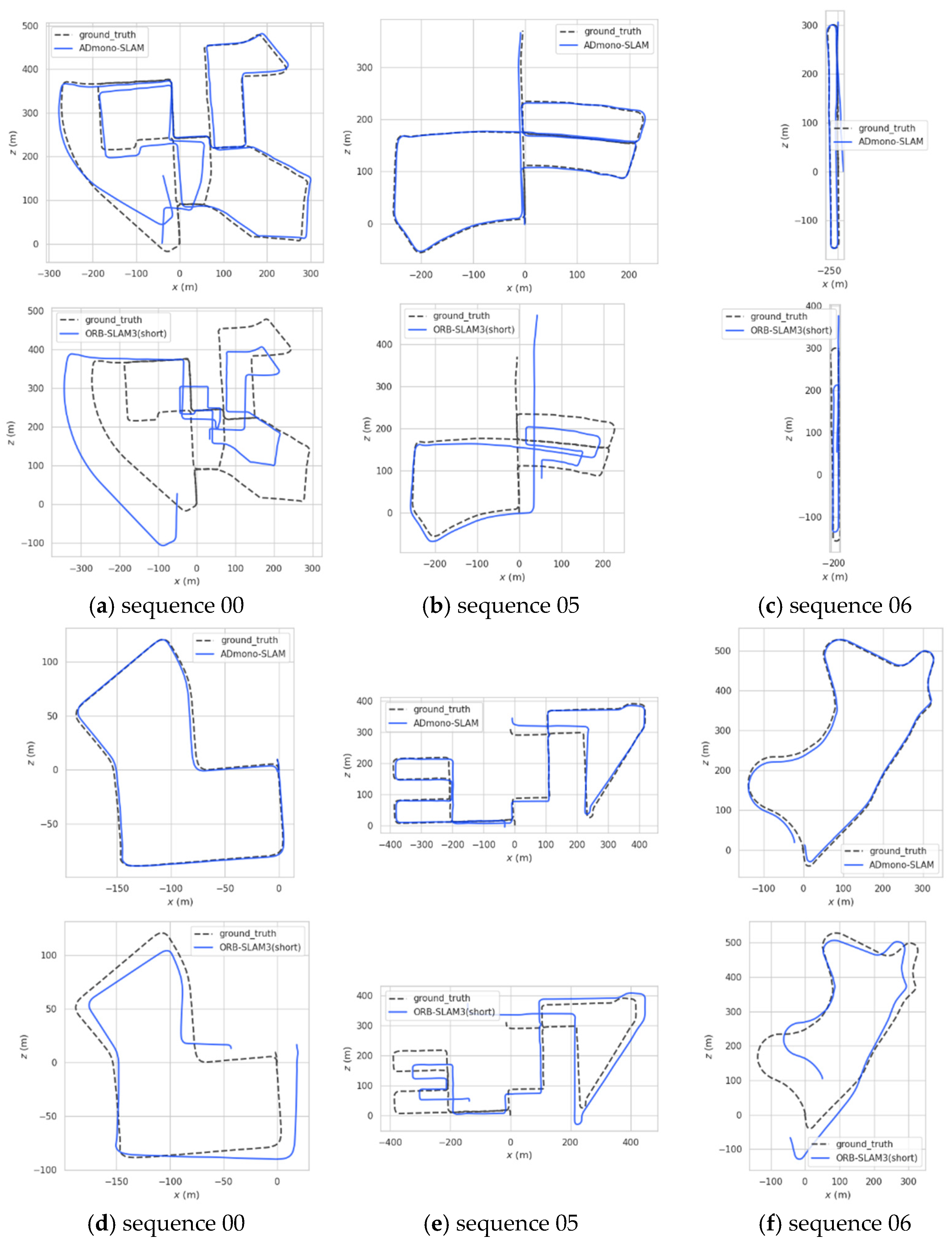
In order to qualitatively analyze the trajectory results of our approach, a trajectory comparison of ADEmono-SLAM and ORB-SLAM3 (short version) was carried out on sequences 00, 05, 06, 07, 08, and 09. The results are shown in Figure 6. The gray dotted line represents the real trajectory, and the blue line represents the method of comparison. Figure 6a–f show the trajectory of sequences 00, 05, 06, 07, 08, and 09. The upper row in each subplot represents the trajectory of ADEmono-SLAM. The second row in each subplot represents the trajectory of ORB-SLAM3 (short version). From these results, ADEmono-SLAM is obviously closer to the real trajectory than ORB-SLAM3 (short version), which implies that the proposed approach has quite good robustness.
To further validate the performance of our approach, we compared ADEmono-SLAM with the popular deep learning methods ESP-VO [17], UndeepVO [18], LSTM-VO [19], DSOD [23], DeepAVO [22], RAUM-VO [20], and TSformer-VO [21]. Among these methods, ESP-VO applies recurrent convolutional networks for probabilistic visual odometry. UndeepVO recovers scale using unsupervised deep learning. LSTM-VO leverages recurrent neural networks for motion learning. DSOD integrates semantic segmentation with direct methods. DeepAVO refines pose with feature distillation. RAUM-VO adjusts rotation via epipolar constraints. TSformer-VO employs transformers for feature extraction. The results are shown in Table 2. t_rel denotes the average translational RMSE drift (%) at a length of 100 m–800 m. r_rel represents the average rotational RMSE drift (°/100 m) at a length of 100 m–800 m. The best results are highlighted in bold. ‘-’ denotes that the paper did not provide experimental results.
On sequence 03, 05, 06, 07, 08, and 10, the average translational RMSE drift of ADEmono-SLAM is 2.55, 1.73, 1.89, 1.51, 2.97, and 2.09, respectively, which is obviously lower than other deep learning methods. For sequence 00, 02, and 09, ADEmono-SLAM achieved the second-lowest accuracy. Specifically, the average translational RMSE drift of ADEmono-SLAM is 3.20, 3.58, and 3.09, which is slightly higher than RAUM-VO, which achieved the lowest t_rel. However, ADmono-SLAM achieved the lowest average value of t_rel among these methods.
For average rotational RMSE drift, ADmono-SLAM achieved the best results on sequences 02, 03, 05, 06, 07, 08, and 10. Specifically, the rrel is 0.47, 0.27, 0.33, 0.60, 0.31, 0.44, and 0.44, respectively, for these sequences. The RAUM-VO method achieved the best rrel values on sequence 00 and 09 at 0.77 and 0.31, respectively. The reason may be that RAUM-VO is a frame-to-frame motion estimation method based on a model-free epipolar constraint, which can utilize deep networks to match 2D keypoints between consecutive frames, while training the network for depth and pose estimation using an unsupervised training protocol. However, the average rrel is 0.46 on all sequence images, which is obviously lower than the other methods.
We then measured the absolute translation RMSE for three popular methods on all sequence images. The tabs of ADmono-SLAM is 5.18, 4.33, 2.21, 14.5, and 4.06 on sequence 05, 06, 07, 08, and 10, respectively, which is lower than the other methods. RAUM-VO achieved the lowest tabs on sequence 00, 02, 03, and 09. The reason may be the good performance of RAUM-VO in addressing issues such as scale drift and degeneracy motion. The average tabs of ADmono-SLAM is 9.72, which is also the best result among these methods. From above experimental results, ADEmono-SLAM tended to achieve the lowest average error across most sequences, which suggests that the proposed method outperforms both end-to-end and hybrid approaches.

4.2. Experiments on TUM RGBD Dataset

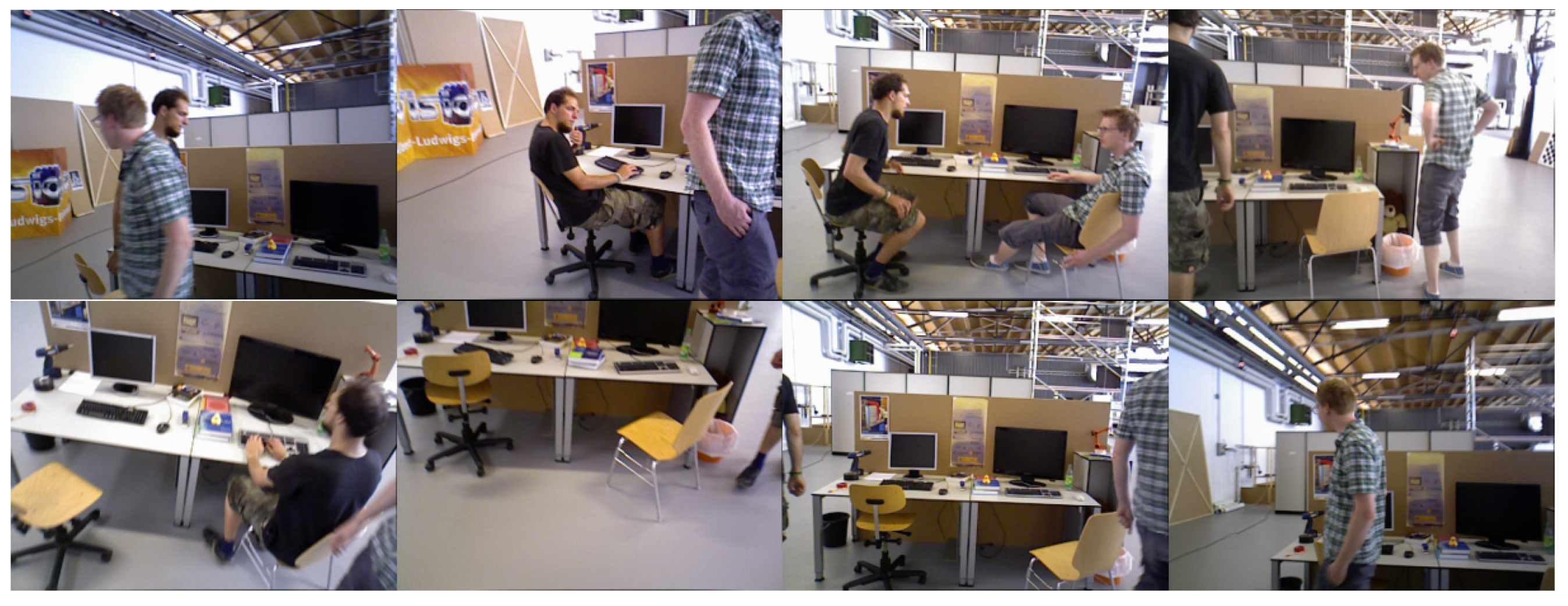
The TUM RGBD dataset contains indoor RGB images and depth maps at a resolution of 640 × 480 [7]. This dataset includes sequences with handheld motion, robot motion, dynamic objects, and validation files. Four image sequences were used in our experiments. In sequence freiburg3_walking_static, two persons walk through an office scene. The Asus Xtion sensor (AsusTek Computer Inc., Taipei, Taiwan, China) is kept in place manually. This sequence is intended to evaluate the robustness of visual SLAM and odometry algorithms to quickly moving dynamic objects in large parts of the visible scene. In sequence freiburg3_walking_xyz, two persons walk through an office scene. The Asus Xtion sensor is manually moved along three directions (xyz) while keeping the same orientation. This sequence is intended to evaluate the robustness of visual SLAM and odometry algorithms to quickly moving dynamic objects in large parts of the visible scene. In sequence freiburg3_walking_halfsphere, two persons walk through an office scene. The Asus Xtion sensor is moved on a small half-sphere of approximately one meter diameter. This sequence is intended to evaluate the robustness of visual SLAM and odometry algorithms to quickly moving dynamic objects in large parts of the visible scene. In sequence freiburg3_walking_rpy, two persons walk through an office scene. The Asus Xtion sensor is rotated along the principal axes (roll–pitch–yaw) at the same position. This sequence is intended to evaluate the robustness of visual SLAM and odometry algorithms to quickly moving dynamic objects in large parts of the visible scene. Some typical images are shown in Figure 7.
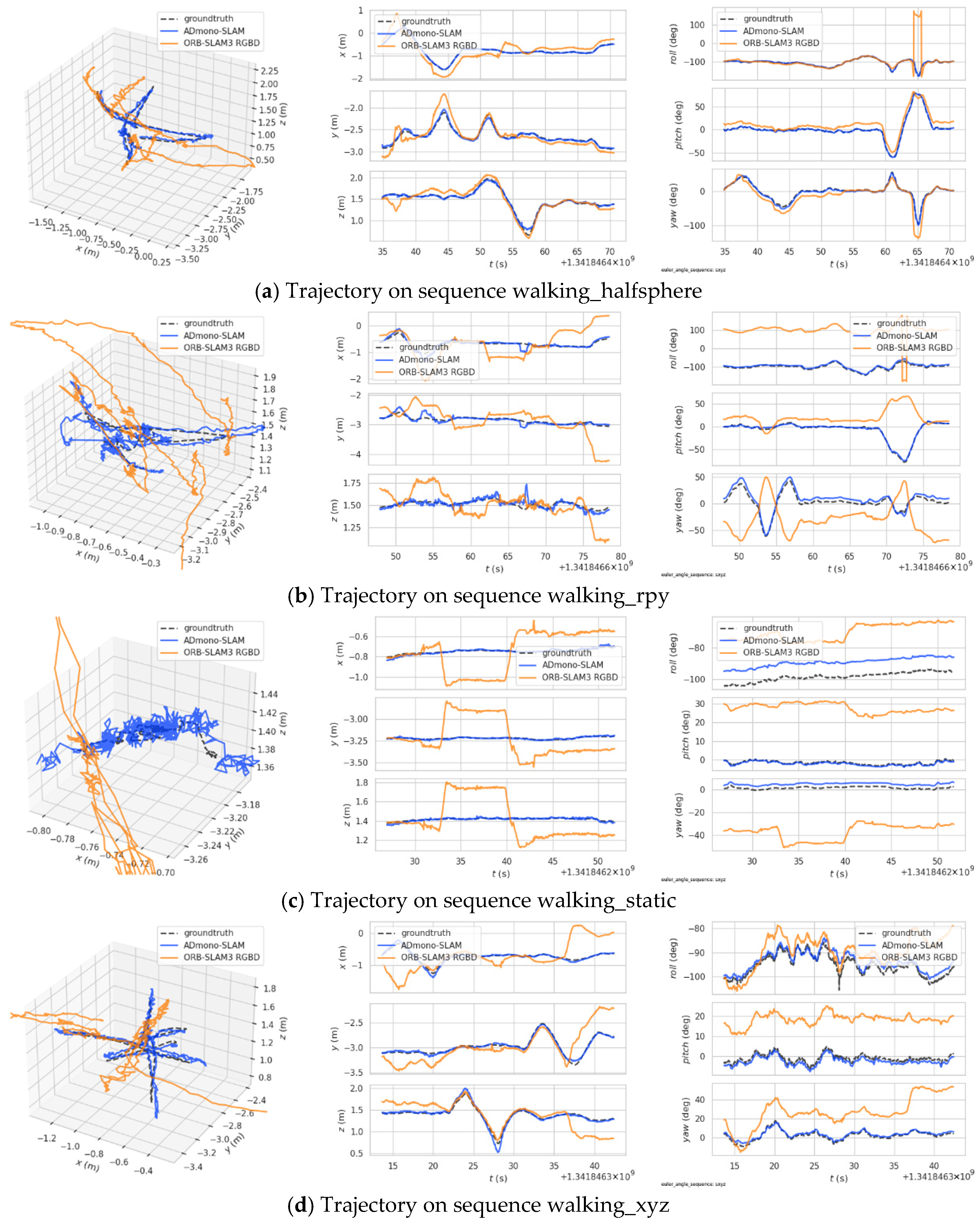
Dynamic scene sequences were selected to compare ADEmono-SLAM with popular ORB-SLAM3 RGBD [19]. We employed absolute translation RMSE to evaluate performance. The trajectories of both methods are not scaled, and neither has loop closure detection. Table 3 shows some comparison results for the TUM RGBD dataset. The tabs of ADEmono-SLAM on sequence walking_halfsphere, walking_rpy, walking_static, and walking_xyz is 0.043, 0.109, 0.014, and 0.066, respectively. These experimental values are typically lower than ORB-SLAM3 RGBD. Basically, ADEmono-SLAM reduces error by at least 80% compared with ORB-SLAM3 RGBD. The comparison results suggest that ADEmono-SLAM has excellent performance in tracking the trajectories of dynamic targets.
Some qualitative comparisons are illustrated in Figure 8. In these experiments, our approach remains close to the ground truth even in the presence of dynamic interference. At the same time, each sequence includes a comparison of camera motion trajectories, variations in camera coordinates over time, and changes in camera Euler angles. The yellow curve represents ORB-SLAM3 RGBD, the blue curve represents ADEmono-SLAM, and the gray dotted line represents the real trajectory. The leftmost sub-figure of each graph represents the comparison of camera trajectories, the middle sub-figure shows the changes in camera coordinates over time, and the rightmost sub-figure illustrates the changes in camera Euler angles over time. From the three comparative figures of each sequence, it can be seen that the ORB-SLAM3 RGB-D method experiences significant drift, both in static and dynamic states, whereas the algorithm presented in this paper maintains strong robustness against interference, even in the presence of multiple dynamic objects, and the computation of camera pose is more accurate and stable. The experimental results suggest that ADEmono-SLAM involving dynamic interference suppression can not only effectively perform feature point detection, but also remove dynamic features. This mechanism is able to effectively improve robustness in dynamic environments. This also indicates that dynamic interference point removal is very important, as various types of dynamic interference exist in real-world environments, which can reduce system robustness.
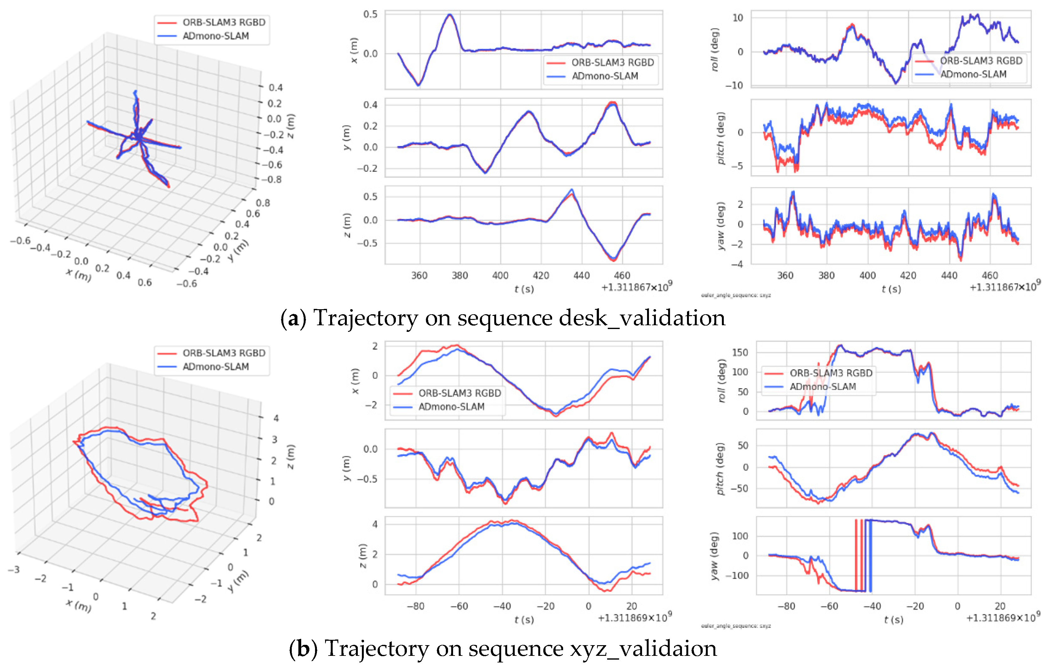
To further verify scale stability, validation sequences without ground-truth trajectories from the TUM RGB-D dataset were selected for testing. The experimental results are shown in Figure 9. The red curve represents ORB-SLAM3 RGBD, and the blue curve represents ADEmono-SLAM. The leftmost sub-figure of each graph represents the comparison of camera trajectories, the middle sub-figure shows the changes in camera coordinates over time, and the rightmost sub-figure illustrates the changes in camera Euler angles over time. It is not difficult to conclude from the six comparative figures that, without any scaling of the trajectories, the scales of the two trajectories are similar, which indicates that the scale of the method proposed in this paper has good determinacy and stability. The reason is that ADEmono-SLAM incorporating an absolute depth estimation network is able to resolve the inherent scale ambiguity of monocular vision and significantly reduces scale drift in long-distance motion. By changing the camera’s coordinate position and Euler angles, the issue of simulating target scale uncertainty is expected to be addressed. Despite changes in target scale, ADEmono-SLAM was still able to achieve stable trajectories, indicating that the absolute depth estimation network played a significant role. The experimental results reveal that ADEmono-SLAM maintains consistent scale compared with ORB-SLAM3 RGBD.

4.3. Experiments on Mobile Robot Platform

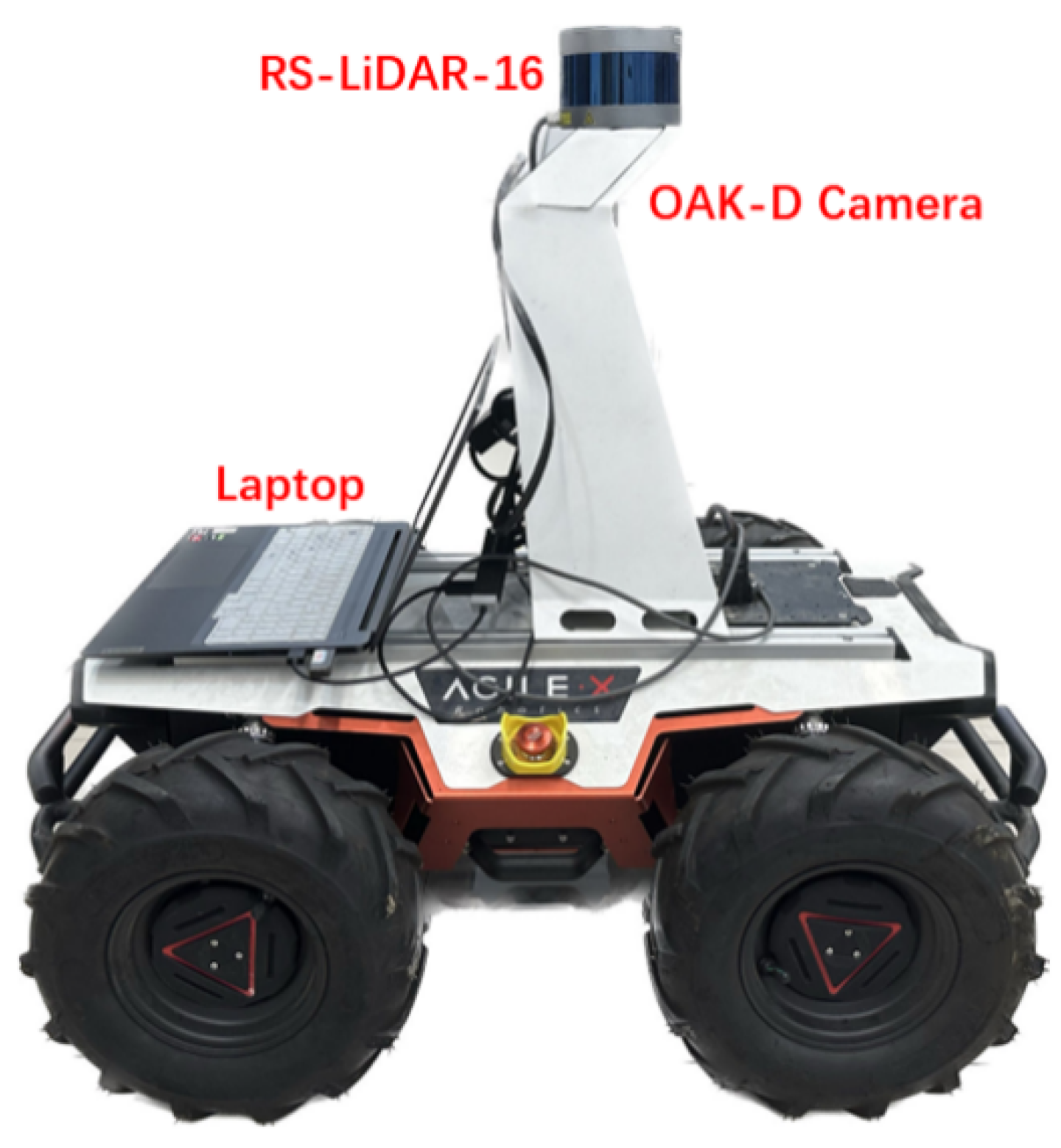
To further validate the generalization ability of the proposed approach beyond public benchmarks, we built a mobile robot platform (shown in Figure 10). We implemented the ADEmono-SLAM algorithm on the mobile robot platform. The mobile robot platform is equipped with an OAK-D RGB camera (Luxonis, Pittsburgh, PA, USA) (640 × 360, 5–6 Hz), an RS-LiDAR-16 sensor (RoboSense, Shenzhen, Guangdong, China) (10 Hz) for ground-truth acquisition, and a laptop with an AMD Ryzen 7 5800H processor (Advanced Micro Devices, Inc., Santa Clara, CA, USA) (3.1 GHz) and 16 GB RAM. Ground-truth trajectories are generated using Lego-LOAM [43]. RGB images are captured using an OAK-D camera with a Sony IMX378 RGB module (Sony Semiconductor Solutions Corporation, Tokyo, Japan) (12 MP) and built-in Myriad X vector processing unit (VPU) for edge vision processing. Though only RGB monocular input is used, calibrated intrinsic and distortion parameters ensure reliable depth estimation and reconstruction. High-precision 6 degrees of freedom (6DoF) trajectories generated by a Robosense RS-LiDAR-16 (RoboSense, Shenzhen, Guangdong, China) combined with the Lego-LOAM algorithm serve as ground truth. Lego-LOAM, widely used for laser SLAM truth acquisition due to its robustness and real-time performance, enabled the validation of our method’s localization accuracy in large dynamic scenes via visual–laser trajectory comparisons.
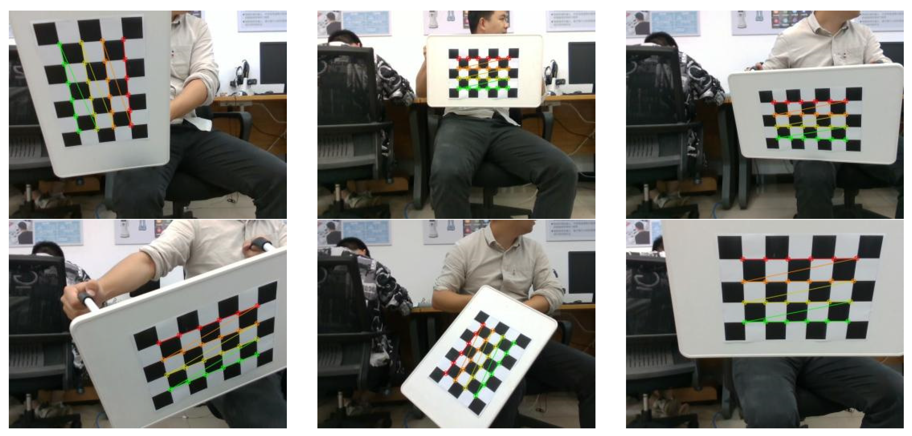
The mobile robot platform can provide a reproducible system for integrating absolute depth estimation with SLAM in both indoor and outdoor scenarios. This setup demonstrates the feasibility of deploying the proposed system in real-world conditions, bridging the gap between simulation and practice. Camera intrinsic parameter calibration was performed using the calibration functions included in OpenCV library 4.5.1, by capturing multiple images of a 7 × 5 chessboard and taking the average. Some images after capturing and calibration processing are shown in Figure 11.
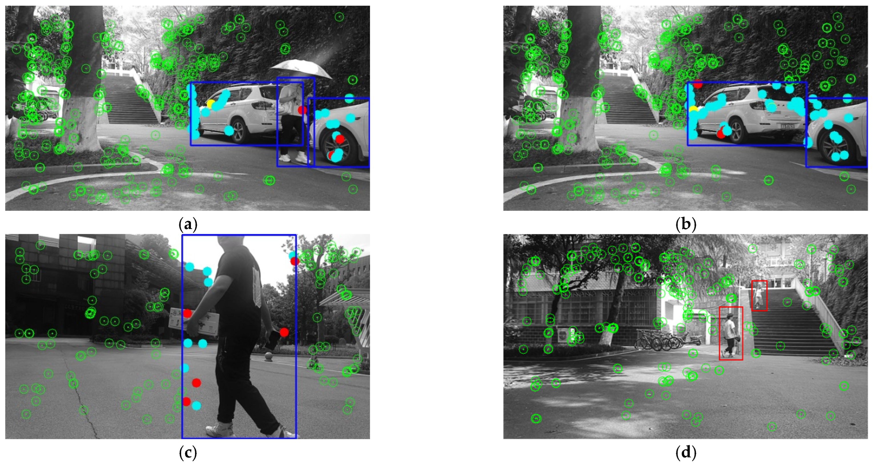
To quantitatively assess the contribution of dynamic removal to SLAM localization and mapping quality, evaluate the impact of long-distance filtering on localization, and analyze the interaction between the two modules, some ablation experiments were conducted using the mobile robot platform. Figure 12 shows the feature point detection results of the method in an outdoor environment, in this figure, the green circles represent key static feature points retained after screening, when a significant number of feature points appear within the bounding box of potential dynamic objects, the moving feature points are recognized as dynamic points, while the feature points in the background are static points. Figure 12a shows that when both static and dynamic objects appear in the scene (vehicles at rest and pedestrians in motion), most of the feature points extracted from static objects are identified as static points (light blue points), while dynamic targets can still detect dynamic points (red points), even if they have fewer feature points. Figure 12b presents the feature point detection results for static objects, where it can be seen that a large number of feature points are detected in the static vehicle area. Figure 12c shows the feature point detection results for dynamic targets; when a significant number of feature points appear within the bounding box of potential dynamic objects, the moving feature points are recognized as dynamic points, while the feature points in the background are static points. Figure 12d illustrates that when small dynamic objects are present, regardless of whether these objects are in motion or at rest, all feature points need to be eliminated. In real scenarios, some small dynamic points are long-range feature points, and these long-range feature points are relatively less important for trajectory generation. ADEmono-SLAM involving a probabilistic distant feature filtering module has noise-aware selectivity in terms of long-distance points, which can significantly balance noise suppression and feature completeness.
The quantitative results for the absolute translation RMSE are summarized in Table 4. The tabs of ADEmono-SLAM is 0.381 and 1.209 in the indoor and outdoor environment, respectively. ORB-SLAM3 RGBD achieved 0.419 and 2.165 of tabs, respectively. From this result, ADEmono-SLAM achieves comparable accuracy to ORB-SLAM3 (short) [43] and significantly outperforms it in the outdoor dataset, where long-distance feature filtering becomes critical. Further, we measured the trajectory accuracy using ADEmono-SLAM without the dynamic interference point removal module and long-distance point filtering module. The tab of ADEmono-SLAM without dynamic interference point removal is 0.507 and 1.986. ADEmono-SLAM without long-distance point filtering achieved tabs values of 0.466 and 2.372, respectively. When dynamic interference point removal and long-distance point filtering are not used, the tabs is quite high at 1.131 and 4.625, respectively.
From the ablation experiments, dynamic removal should significantly reduce absolute errors and map noise in high-dynamic scenarios. However, if it is too aggressive, it may inadvertently delete static features, leading to incomplete maps or degraded localization. In scenes with long-distance noise, long-distance filtering can improve matching stability and reduce computational costs, but filtering too many stable features at long distances can impair relocalization ability. The two modules are complementary in most scenarios, but in close-range situations, the impact of long-distance filtering may be minimal, requiring adaptive switching or threshold adjustments based on the scene.
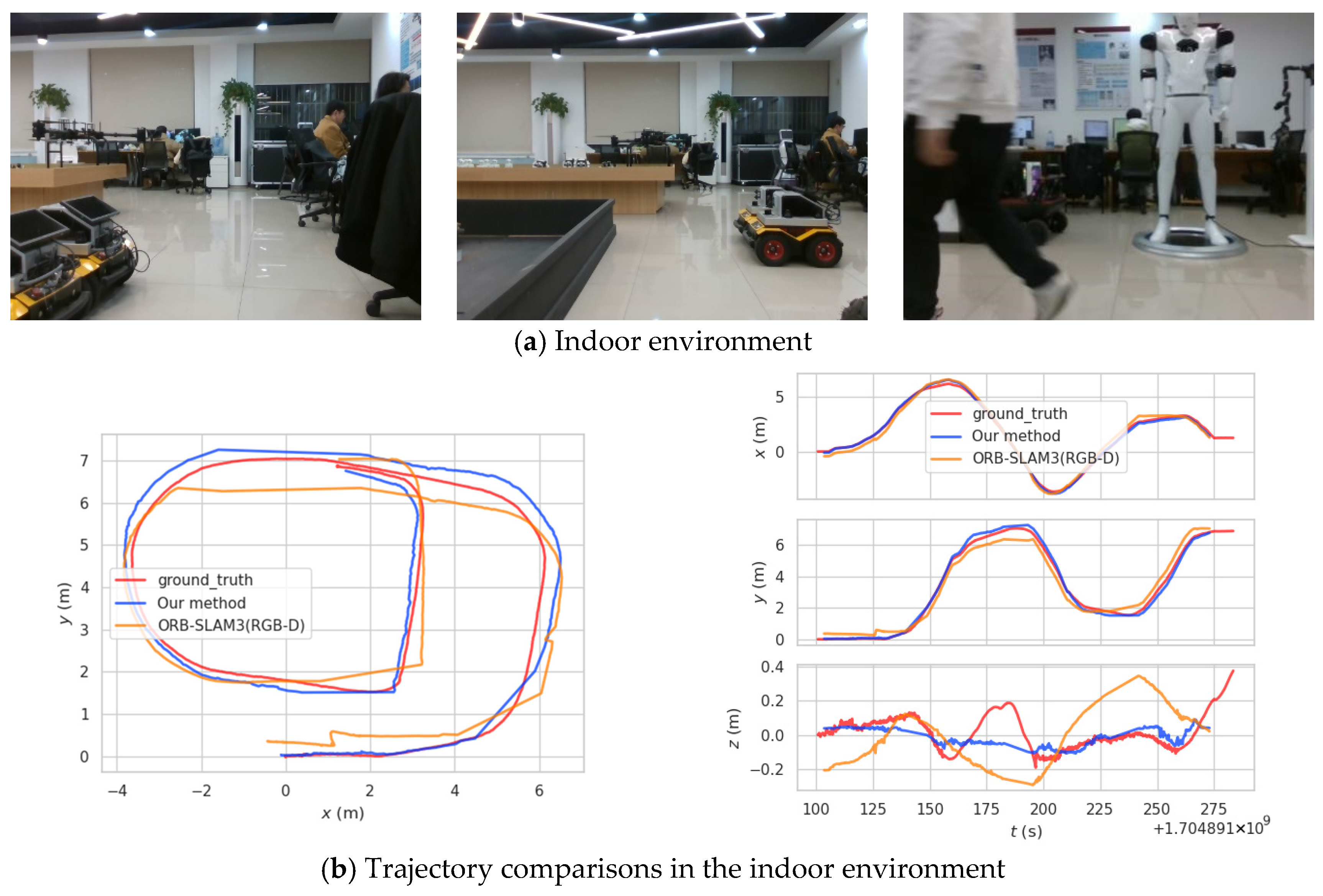
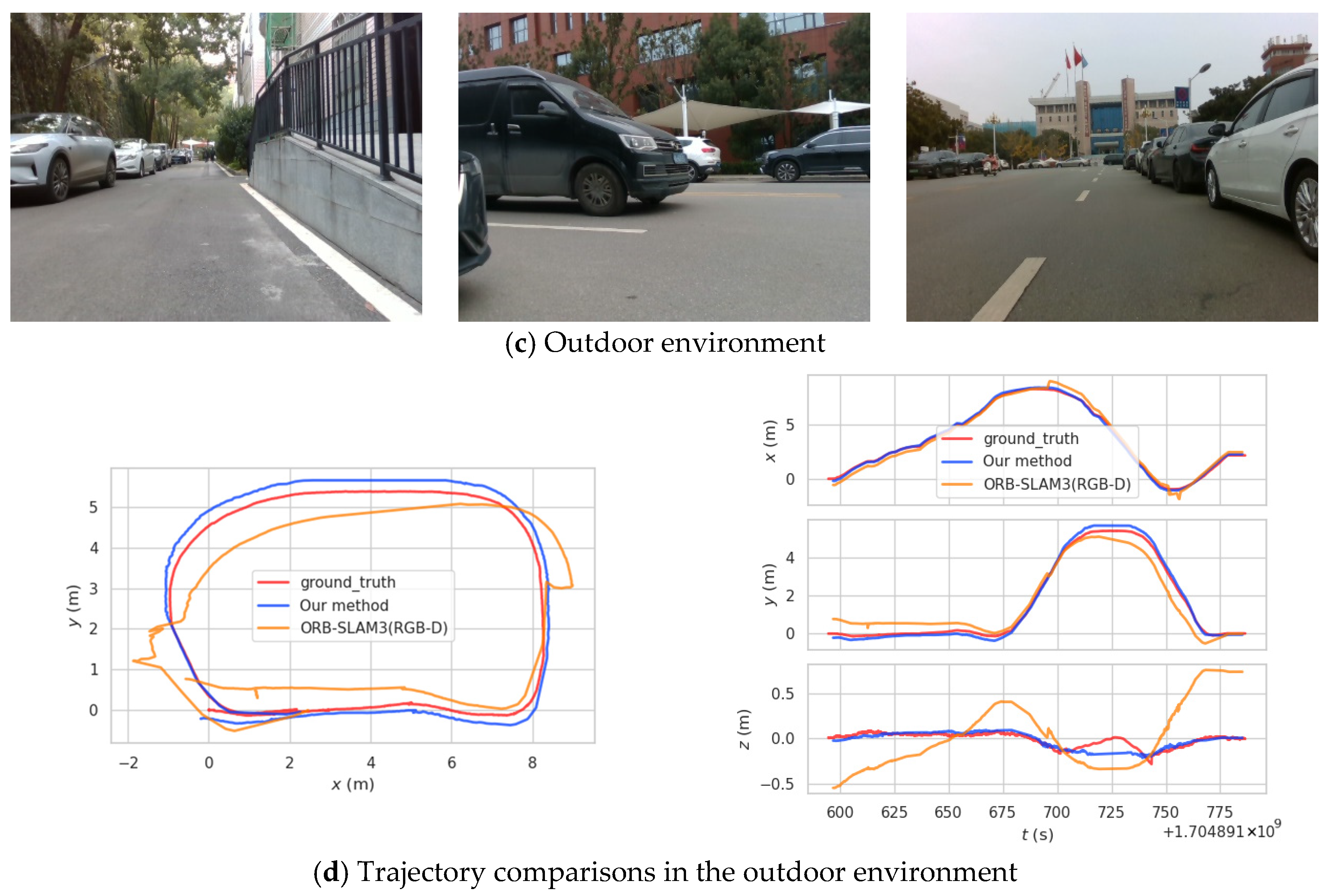
To provide a more intuitive comparison, Figure 13 displays the trajectory comparisons of two algorithms in indoor and outdoor environments without scaling. Figure 13a shows the indoor environment image, while Figure 13b’s left column presents the comparison of the ground truth trajectory, the proposed algorithm, and the ORB-SLAM3 planar trajectory. The right column of Figure 13b shows the variation in the camera’s 3D coordinates over time. Figure 13c depicts the outdoor environment image, and Figure 13d’s left column compares the ground truth trajectory, the proposed algorithm, and the ORB-SLAM3 planar trajectory, while the right column of Figure 13d illustrates the change in the camera’s 3D coordinates over time. In the experiments, both comparison algorithms were only aligned with the true trajectory without scaling and did not utilize loop closure detection.
From Figure 13, it can be seen that the planar coordinates of the proposed algorithm are closer to the true trajectory, while the trajectory of the ORB-SLAM3 algorithm is significantly affected by the environment, resulting in considerable deviation and frequent jitter. Furthermore, the x-axis and y-axis coordinates of the proposed algorithm remain highly consistent with the true values. Notably, due to the laboratory floor being level without significant height differences, there are even drifts in the true values along the z-axis, while the proposed algorithm demonstrates a relatively smooth performance, remaining at around 0 m throughout the process.
We also measured the runtime of our approach on the mobile robot platform. The absolute depth estimation network can process images at a speed of 15 frames per second, which is almost real-time computational efficiency. The time of YOLOv5 detection is 100 ms for a 640 × 360 image. The ORB feature extraction algorithm uses the rotation-invariant BRIEF descriptor to generate binary strings by comparing the grayscale values of pixel pairs in the neighborhood of feature points. Therefore, the ORB feature extraction algorithm is very fast, with a computation time of about 10 ms for a 640 × 360 image. Basically, all of the algorithms can meet real-time SLAM requirements.

5. Conclusions

In this paper, we addressed the problems of scale uncertainty and dynamic environment interference in monocular SLAM. We proposed the ADEmono-SLAM approach that integrates an absolute depth estimation network with geometric optimization. The integration of an object detection network enables dynamic interference removal, enhancing system stability in complex scenarios. A long-distance feature point filtering strategy was designed to improve feature matching quality and back-end optimization robustness. Experimental results on both public datasets and mobile robot platform demonstrate that ADEmono-SLAM can usually achieve quite good performance, while showing significant advantages in large-scale environments. Although the proposed method can handle dynamic interference targets and trajectory generation tasks with partial occlusion, its robustness under special visual conditions such as reflections, transparent surfaces, and complex occlusions still needs to be verified. Furthermore, ADEmono-SLAM includes modules for absolute depth estimation, dynamic interference removal, and long-distance feature point filtering, but the integrated optimization framework requires further design to better validate its feasibility for application on embedded platforms.

Author Contributions

Conceptualization, K.Z.; methodology, X.Z.; software, P.T. and H.L.; validation, Z.Y. and Y.Y.; writing—original draft preparation, P.T.; manuscript revision, H.L.; writing—review and editing, visualization, H.L., Z.Y. and Y.Y. All authors have read and agreed to the published version of the manuscript.

Funding

This work was partly supported by the Major Program of Xiangjiang Laboratory (23XJ01009, 22XJ01002).

Data Availability Statement

The original contributions presented in this study are included in the article.

Conflicts of Interest

The authors declare no conflicts of interest.

References

  1. Durrant-Whyte, H.; Bailey, T. Simultaneous localization and mapping: Part I. IEEE Robot. Autom. Mag. 2006, 13, 99–110. [Google Scholar] [CrossRef]
  2. Bailey, T.; Durrant-Whyte, H. Simultaneous localization and mapping (SLAM): Part II. IEEE Robot. Autom. Mag. 2006, 13, 108–117. [Google Scholar] [CrossRef]
  3. Fuentes-Pacheco, J.; Ruiz-Ascencio, J.; Rendon-Mancha, J.M. Visual simultaneous localization and mapping: A survey. Artifificial Intell. Rev. 2015, 43, 55–81. [Google Scholar] [CrossRef]
  4. Chen, Y.; Zhou, Y.; Lv, Q.; Deveerasetty, K.K. A review of V-SLAM. In Proceedings of the 2018 IEEE International Conference on Information and Automation (ICIA), Wuyishan City, China, 11–13 August 2018; IEEE: New York, NY, USA, 2018; pp. 603–608. [Google Scholar]
  5. Gao, X.; Zhang, T. The Fourteen Lectures on Visual SLAM; Publishing House of Electronics Industry: Beijing, China, 2017; pp. 16–18. [Google Scholar]
  6. Geiger, A.; Lenz, P.; Urtasun, R. Are we ready for autonomous driving? The KITTI vision benchmark suite. In Proceedings of the 2012 IEEE Conference on Computer Vision and Pattern Recognition, Providence, RI, USA, 16–21 June 2012; IEEE: New York, NY, USA, 2012; pp. 3354–3361. [Google Scholar]
  7. Sturm, J.; Engelhard, N.; Endres, F.; Burgard, W.; Cremers, D. A benchmark for the evaluation of RGB-D SLAM systems. In Proceedings of the 2012 IEEE International Conference on Intelligent Robots and Systems, Vilamoura-Algarve, Portugal, 7–12 October 2012; pp. 573–580. [Google Scholar]
  8. Davison, A.J.; Reid, I.D.; Molton, N.D.; Stasse, O. MonoSLAM: Real-Time Single Camera SLAM. IEEE Trans Pattern Anal. Mach. Intell. 2007, 29, 1052–1067. [Google Scholar] [CrossRef]
  9. Klein, G.; Murray, D. Parallel Tracking and Mapping for Small AR Workspaces. In Proceedings of the IEEE International Symposium on Mixed & Augmented Reality, Cambridge, UK, 15–18 September 2008. [Google Scholar]
  10. Mur-Artal, R.; Montiel, J.M.M.; Tardos, J.D. ORB-SLAM: A versatile and accurate monocular SLAM system. IEEE Trans. Robot. 2015, 31, 1147–1163. [Google Scholar] [CrossRef]
  11. Mur-Artal, R.; Tardós, J.D. ORB-SLAM2: An open-source SLAM system for monocular, stereo, and RGB-D cameras. IEEE Trans. Robot. 2017, 33, 1255–1262. [Google Scholar] [CrossRef]
  12. Campos, C.; Elvira, R.; Rodríguez, J.J.G.; Montiel, J.M.M.; Tardos, J.D. ORB-SLAM 3: An accurate open-source library for visual, visual–inertial, and multimap SLAM. IEEE Trans. Robot. 2021, 37, 1874–1890. [Google Scholar] [CrossRef]
  13. Engel, J.; Koltun, V.; Cremers, D. Direct sparse odometry. IEEE Trans. Pattern Anal. Mach. Intell. 2017, 40, 611–625. [Google Scholar] [CrossRef]
  14. Qi, L.; Wang, R.; Hu, C.; Li, S.; Xu, X. Time-Aware Distributed Service Recommendation with Privacy-Preservation. Inf. Sci. 2018, 480, 354–364. [Google Scholar] [CrossRef]
  15. Lu, Y.W.; Lu, G.Y. An unsupervised approach for simultaneous visual odometry and single image depth estimation. In Proceedings of the 2022 International Joint Conference on Neural Networks (IJCNN), Padua, Italy, 18–23 July 2022. [Google Scholar]
  16. Wang, S.; Clark, R.; Wen, H.; Trigoni, N. Deepvo: Towards end-to-end visual odometry with deep recurrent convolutional neural networks. In Proceedings of the 2017 IEEE International Conference on Robotics and Automation (ICRA), Singapore, 29 May–3 June 2017; IEEE: New York, NY, USA, 2017; pp. 2043–2050. [Google Scholar]
  17. Wang, S.; Clark, R.; Wen, H.; Trigoni, N. End-to-end, sequence-to-sequence probabilistic visual odometry through deep neural networks. Int. J. Robot. Res. 2018, 37, 513–542. [Google Scholar] [CrossRef]
  18. Li, R.; Wang, S.; Long, Z.; Gu, D. Undeepvo: Monocular visual odometry through unsupervised deep learning. In Proceedings of the 2018 IEEE International Conference on Robotics and Automation (ICRA), Brisbane, Australia, 21–25 May 2018; IEEE: New York, NY, USA, 2018; pp. 7286–7291. [Google Scholar]
  19. Zhao, C.Q.; Yen, G.G.; Sun, Q.Y.; Zhang, C.Z.; Tang, Y. Masked GAN for unsupervised depth and pose prediction with scale consistency. IEEE Trans. Neural Netw. Learn. Syst. 2021, 32, 5392–5403. [Google Scholar] [CrossRef] [PubMed]
  20. Cimarelli, C.; Bavle, H.; Sanchez-Lopez, J.L.; Voos, H. RAUM-VO: Rotational Adjusted Unsupervised Monocular Visual Odometry. Sensors 2022, 22, 2651. [Google Scholar] [CrossRef] [PubMed]
  21. Françani, A.O.; Maximo, M.R.O.A. Transformer-based model for monocular visual odometry: A video understanding approach. arXiv 2023, arXiv:2305.06121. [Google Scholar] [CrossRef]
  22. Zhu, R.; Yang, M.; Liu, W.; Song, R.; Yan, B.; Xiao, Z. DeepAVO: Efficient pose refining with feature distilling for deep visual odometry. Neurocomputing 2022, 467, 22–35. [Google Scholar] [CrossRef]
  23. Ma, P.; Bai, Y.; Zhu, J.; Wang, C.; Peng, C. DSOD: DSO in dynamic environments. IEEE Access 2019, 7, 178300–178309. [Google Scholar] [CrossRef]
  24. Bhat, S.F.; Birkl, R.; Wofk, D.; Wonka, P.; Muller, M. Zoedepth: Zero-shot transfer by combining relative and metric depth. arXiv 2023, arXiv:2302.12288. [Google Scholar]
  25. Liang, W.; Chen, X.H.; Huang, S.; Xiong, G.; Yan, K.; Zhou, X. Federated Learning Edge Network Based Sentiment Analysis Combating Global COVID-19. Comput. Commun. 2023, 204, 33–42. [Google Scholar] [CrossRef]
  26. Zhou, X.; Zheng, X.; Cui, X.; Shi, J.; Liang, W.; Yan, Z.; Yang, L.T.; Shimizu, S.; Wang, K.I.-K. Digital Twin Enhanced Federated Reinforcement Learning with Lightweight Knowledge Distillation in Mobile Networks. IEEE J. Sel. Areas Commun. 2023, 41, 3191–3211. [Google Scholar] [CrossRef]
  27. Meng, F.; Chen, X.H. Generalized Archimedean Intuitionistic Fuzzy Averaging Aggregation Operators and Their Application to Multicriteria Decision-Making. Int. J. Inf. Technol. Decis. Mak. 2016, 15, 1437–1463. [Google Scholar] [CrossRef]
  28. Zhang, P.; Wang, J.; Li, W. A Learning Based Joint Compressive Sensing for Wireless Sensing Networks. Comput. Netw. 2020, 168, 107030. [Google Scholar] [CrossRef]
  29. Ranftl, R.; Lasinger, K.; Hafner, D.; Schindler, K.; Koltun, V. Towards robust monocular depth estimation: Mixing datasets for zero-shot cross-dataset transfer. IEEE Trans. Pattern Anal. Mach. Intell. 2020, 44, 1623–1637. [Google Scholar] [CrossRef] [PubMed]
  30. Zou, Y.; Ji, P.; Tran, Q.H.; Huang, J.-B.; Chandraker, M. Learning Monocular Visual Odometry via Self-Supervised Long-Term Modeling; ECCV 2020; Springer: Berlin/Heidelberg, Germany, 2020; pp. 710–727. [Google Scholar]
  31. Wang, Q.; Zhang, H.; Liu, Z.; Li, X. Information Theoretic Learning-Enhanced Dual-Generative Adversarial Networks with Causal Representation for Robust OOD Generalization. IEEE Trans. Neural Netw. Learn. Syst. 2023, 34, 1632–1646. [Google Scholar]
  32. Wightman, R. Pytorch image models. Available online: https://github.com/liyanhui607/rwightman_pytorch-image-models (accessed on 10 April 2024).
  33. Bhat, S.F.; Alhashim, I.; Wonka, P. LocalBins: Improving Depth Estimation by Learning Local Distributions. In Proceedings of the ECCV 2022: 17th European Conference, Tel-Aviv, Israel, 23–27 October 2022. [Google Scholar]
  34. Zhang, L.; Li, H.; Wang, Q. Point-by-point feature extraction of artificial intelligence images based on the internet of things. Comput. Commun. 2020, 155, 1–9. [Google Scholar]
  35. Qi, L.; Zhang, X.; Dou, W.; Hu, C.; Yang, C.; Chen, J. A Two-Stage Locality-Sensitive Hashing Based Approach for Privacy-Preserving Mobile Service Recommendation in Cross-Platform Edge Environment. Future Gener. Comput. Syst. 2018, 88, 636–643. [Google Scholar] [CrossRef]
  36. Chen, Z.S.; Chen, J.Y.; Chen, Y.H.; Yang, Y.; Jin, L.; Herrera-Viedma, E.; Pedrycz, W. Large-Group Failure Mode and Effects Analysis for Risk Management of Angle Grinders in the Construction Industry. Inf. Fusion 2023, 97, 101803. [Google Scholar] [CrossRef]
  37. Rahima, K.; Muhammad, H. What is YOLOv5: A deep look into the internal features of the popular object detector. arXiv 2024, arXiv:2407.20892. [Google Scholar] [CrossRef]
  38. Zhou, X.; Li, Y.; Liang, W. CNN-RNN Based Intelligent Recommendation for Online Medical Pre-Diagnosis Support. IEEE Trans. Comput. Biol. Bioinform. 2021, 18, 912–921. [Google Scholar] [CrossRef]
  39. Lv, P.Q.; Wang, J.K.; Zhang, X.Y.; Shi, C.F. Deep supervision and atrous inception-based U-Net combining CRF for automatic liver segmentation from CT. Sci. Rep. 2022, 12, 16995. [Google Scholar] [CrossRef]
  40. Zhang, J.; Bhuiyan, M.Z.A.; Xu, X.; Hayajneh, T.; Khan, F. Anticoncealer: Reliable Detection of Adversary Concealed Behaviors in EdgeAI-Assisted IoT. IEEE Internet Things J. 2022, 9, 22184–22193. [Google Scholar] [CrossRef]
  41. Zhou, X.; Liang, W.; Yan, K.; Li, W.; Wang, K.I.-K.; Ma, J.; Jin, Q. Edge-Enabled Two-Stage Scheduling Based on Deep Reinforcement Learning for Internet of Everything. IEEE Internet Things J. 2023, 10, 3295–3304. [Google Scholar] [CrossRef]
  42. Liu, C.; Kou, G.; Zhou, X.; Peng, Y.; Sheng, H.; Alsaadi, F.E. Time-Dependent Vehicle Routing Problem with Time Windows of City Logistics with a Congestion Avoidance Approach. Knowl. Based Syst. 2020, 188, 104813. [Google Scholar] [CrossRef]
  43. Shan, T.; Englot, B. Lego-loam: Lightweight and ground-optimized lidar odometry and mapping on variable terrain. In Proceedings of the 2018 IEEE International Conference on Intelligent Robots and Systems (IROS), Madrid, Spain, 1–5 October 2018; IEEE: New York, NY, USA, 2018; pp. 4758–4765. [Google Scholar]
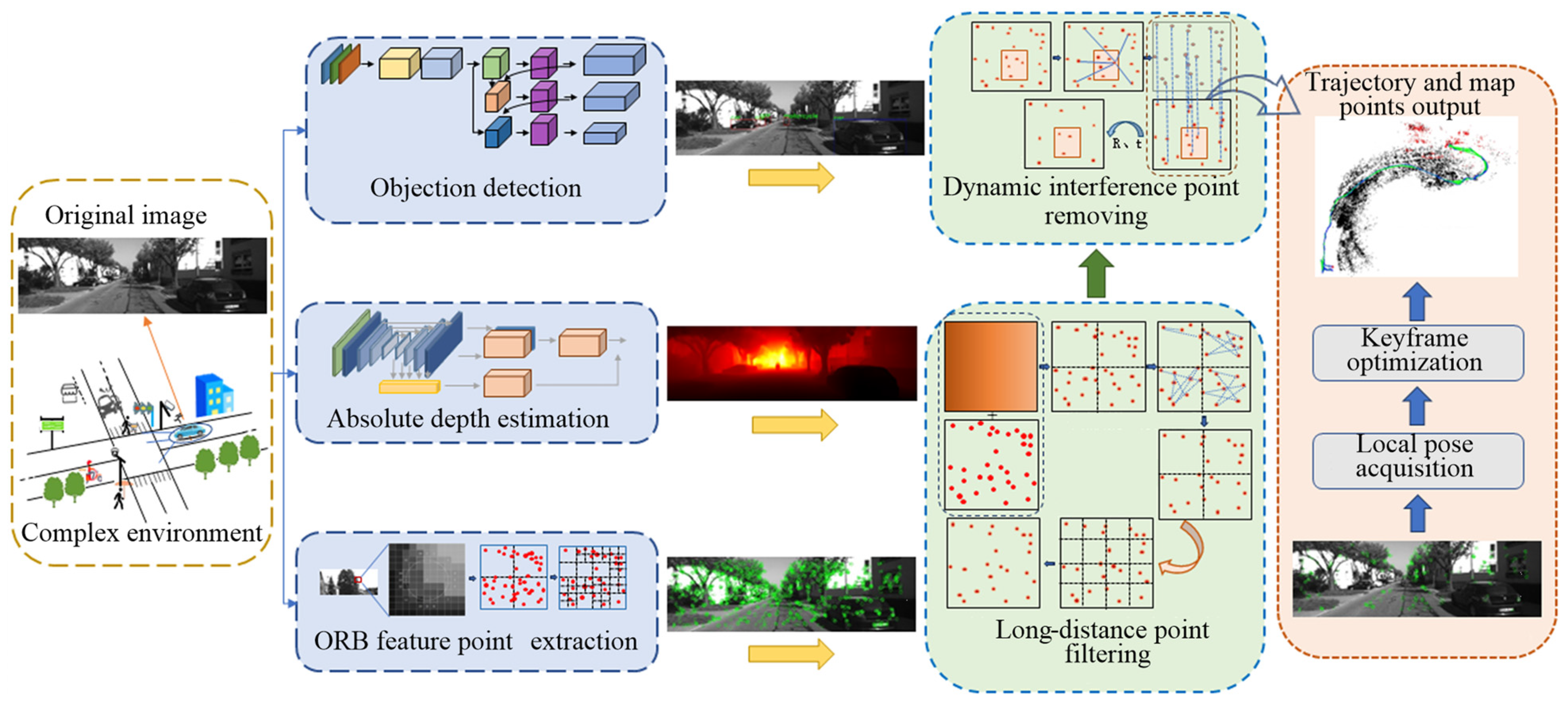
Figure 1. Overall framework of ADEmono-SLAM.
Electronics 14 04126 g001
Figure 2. Framework of the absolute depth estimation network.
Electronics 14 04126 g002
Figure 3. Feature point enhancement algorithm process.
Electronics 14 04126 g003
Figure 4. The processing of dynamic interference point removal. (a) Object detection; (b) different object classification; (c) first stage of interference point removal; (d) second stage of interference point removal.
Electronics 14 04126 g004
Figure 5. KITTI image dataset.
Electronics 14 04126 g005
Figure 6. Trajectory of ADEmono-SLAM and ORB-SLAM3 (short version) on several sequences.
Electronics 14 04126 g006
Figure 7. TUM RGBD dataset.
Electronics 14 04126 g007
Figure 8. Trajectory comparison on four sequences.
Electronics 14 04126 g008
Figure 9. Comparison results on two sequences without real trajectories.
Electronics 14 04126 g009
Figure 10. Mobile robot platform.
Electronics 14 04126 g010
Figure 11. Camera calibration on checkerboard.
Electronics 14 04126 g011
Figure 12. Feature point detection in the outdoor environment. (a) Feature point detection that simultaneously exists for static and dynamic targets; (b) static target feature point detection; (c) feature point detection of dynamic targets; (d) detection of feature points of small dynamic objects.
Electronics 14 04126 g012
Figure 13. The trajectory comparison of the two algorithms.
Electronics 14 04126 g013aElectronics 14 04126 g013b
Table 1. t a b s of several methods on KITTI dataset.
SequenceADEmono-SLAMORB-SLAM3 (Short Version) [12]ORB-SLAM3 (Full Version) [12]ORB-SLAM2 [11]
0020.8981.856.956.20
0222.9938.1727.4729.97
033.701.691.310.97
055.1841.985.275.20
064.3350.6115.0513.27
072.2117.423.171.88
0814.5151.9456.9751.83
099.8857.467.6862.17
104.067.837.337.61
Average t a b s 9.7538.7714.5819.90
Bold values in Table 1 highlight the relatively optimal t a b s results for each sequence or the average among the compared methods, facilitating quick comparison and identification of superior performance.
Table 2. Comparison results of deep learning methods on the KITTI dataset.
MethodSequenceAverage Value
000203050607080910
trel
%
UndeepVO [18]4.145.58-3.40-3.154.08--4.07
ESP-VO [17]--6.723.357.243.52--9.776.12
LSTMVO [19]11.96.91-7.15-8.757.65--8.47
DSOD [23]-15.016.314.414.615.515.113.813.514.7
DeepAVO [22]--3.642.574.963.36--5.494.00
RAUM-VO [20]2.542.573.213.043.032.393.632.925.843.24
TSformer-VO [21]4.644.7312.812.528.922.94.325.4516.012.47
ADmono-SLAM3.203.582.551.731.891.512.973.092.092.51
r r e l ° UndeepVO [18]1.922.44-1.50-2.481.79--2.03
ESP-VO [17]--2.761.211.501.71--2.041.84
LSTMVO [19]4.291.99-2.36-3.541.97--2.83
DeepAVO [22]--1.891.161.342.15--2.491.80
RAUM-VO [20]0.770.581.331.150.831.031.070.310.680.86
TSformer-VO [21]1.891.565.755.138.8311.51.672.085.164.84
ADmono-SLAM0.930.470.270.330.600.310.440.350.440.46
t a b s ( m ) RAUM-VO [20]16.216.12.6017.49.232.1616.38.6612.211.20
TSformer-VO [21]46.555.214.161.388.331.426.423.622.641.04
ADmono-SLAM20.822.93.705.184.332.2114.59.884.069.72
Bold values in the table indicate the best performance among the compared methods for each sequence, facilitating quick identification of optimal results.
Table 3. t a b s on TUM RGBD dataset.
SequenceADEmono-SLAMORB-SLAM3 RGBD [19]
fr3/walking_halfsphere0.0430.319
fr3/walking_rpy0.1090.671
fr3/walking_static0.0140.361
fr3/walking_xyz0.0660.622
Bold values in Table 3 represent the performance values of the proposed ADEmono-SLAM method, which are highlighted to facilitate the quick identification of its superior results compared with ORB-SLAM3 RGBD.
Table 4. t a b s   on mobile robot platform.
MethodIndoor EnvironmentOutdoor Environment
ADEmono-SLAM0.3811.209
ORB-SLAM3 RGBD [19]0.4192.165
ADEmono-SLAM without dynamic interference point removal0.5071.986
ADEmono-SLAM without long-distance point filtering0.4662.372
ADEmono-SLAM without dynamic interference point removal and long-distance point filtering1.1314.625
Bold values in Table 4 represent the performance values of the proposed ADEmono-SLAM method, which are highlighted to facilitate the quick identification of its superior results in different environments compared with other methods or variants.
Disclaimer/Publisher’s Note: The statements, opinions and data contained in all publications are solely those of the individual author(s) and contributor(s) and not of MDPI and/or the editor(s). MDPI and/or the editor(s) disclaim responsibility for any injury to people or property resulting from any ideas, methods, instructions or products referred to in the content.