Abstract
Traditional ISAR imaging algorithms are based on the “stop-and-go” assumption and lack theoretical analysis, accurate simulation, and effective compensation regarding the high-speed motion of the target or the platform. In response to this issue, a theoretical analysis of the high-speed motion of the target or the platform in ISAR imaging is first conducted, indicating that when a chirp is transmitted, the echo from a scatterer can be approximated as a chirp with its central frequency and chirp rate changed, and this will lead to the shift and the blurring of the scatterer in range. A method is then proposed to estimate the central frequency and the chirp rate, which are used to adjust the central frequency and the chirp rate of the matched filter. The central frequency is estimated to maximize the normalized correlation of the amplitude spectrum and its nominal form, and the chirp rate is derived from the central frequency. Moreover, in order to show the rationality of our theoretical analysis and the effectiveness of our compensation method, a scheme is presented to simulate the received signal under the high-speed motion of the target or the platform. This scheme assumes that the target and the platform move continuously with time and reflects the effects of the high-speed motion on the received signal accurately.
1. Introduction
The inverse synthetic aperture radar (ISAR) uses the motion between the radar and the target to image the target. The radar can be ground based, airborne, or space borne. The platform can be stationary or moving. The beam tracks moving targets of interest.
There are various algorithms for ISAR imaging [1]. In this paper, we only discuss the range-Doppler algorithm, which applies to a small rotational angle. For a large rotational angle, typical algorithms include the sub-aperture algorithm, the sub-patch algorithm, the polar-format algorithm, and the back-projection algorithm. Additionally, we assume that the target scene has a rigid projection on the imaging plane. Otherwise, different motion compensations are needed for different targets or different components of a single target. This can be achieved if different targets or different components of a single target can be separated somehow [2,3]. Moreover, we assume that no echoes are missing or damaged in data acquisition. Otherwise, the imaging can be achieved by methods based on Bayesian learning [4,5,6] or deep learning [7,8,9].
The range-Doppler algorithm is the most widely used algorithm for ISAR imaging. First, the scatterers with different ranges are resolved using their differences in time delay. Usually, a wide-band technique, such as the matched-filter technique, the stretch technique, or the stepped-frequency technique, is used to improve range resolution [10,11]. Then, translation compensation is used to remove the effect of the translation between the radar and the target in range. Finally, in each range bin, the scatterers with different azimuths are resolved using their differences in Doppler frequency. The most widely used method is the Fourier transform. Other methods include modern spectral estimation [12] and time-frequency representation [13].
Translation compensation is a key step in ISAR imaging. It usually consists of range alignment and phase adjustment. In range alignment, the signals from the same scatterer are aligned in range by shifting the echoes. If no prior knowledge is available about the translation, range alignment can be achieved using the similarity of the envelopes of the echoes. Typical methods include the peak method [14], the maximum-correlation method [14], the frequency-domain method [14], the Hough-transform method [15], the minimum-entropy method [16], and the global method [17,18]. Phase adjustment is used to remove the translational Doppler phase. Typical methods for phase adjustment include the dominant-scatterer method [14], the scattering-centroid method [11], the phase-gradient method [19,20], the time-frequency method [21], and the sharpest-image method [16,22,23,24,25,26,27,28,29]. These methods apply even if no prior knowledge is available about the translation. Additionally, range alignment and phase adjustment can also be implemented together in the domain of slow time and the frequency in respect to fast time. The minimum-entropy translation compensation, which applies even with no prior knowledge about the translation, is based on this scheme [10].
Recently, with the development of hypersonic equipment, ISAR under the high-speed motion of the target or the platform has received much attention. For example, when dealing with a missile group or an aircraft group, which contains different targets, the ISAR installed on a missile may obtain information about the size and the shape of each target, classify each target, and destroy high-value targets first.
The traditional ISAR imaging algorithms are based on the “stop-and-go” assumption and may not work well when the target or the platform moves at an extremely high speed. Various methods have been presented to compensate for the effects of the high-speed motion in ISAR imaging. These methods can be divided into two categories. One category is based on the parameter estimation of the signal. The parameters of the signal and therefore the velocity of the target to the radar are estimated using the fractional Fourier transform [30,31], the integrating cubic phase functions [32], etc. This category is not robust against noise and target scintillation. The other category is based on the focus quality of the range profile. The chirp rate and therefore the velocity of the target to the radar are estimated by optimizing the focus quality of the range profile [33,34,35]. However, the accuracy of this category is limited because the change of the chirp rate is usually insensitive to the high-speed motion, unlike the central frequency.
This paper studies the effects and the compensation of the high-speed motion of the target or the platform in ISAR imaging. Theoretical analysis shows that when a chirp is transmitted, the echo from a scatterer can be approximated as a chirp with its central frequency and chirp rate changed, and this will lead to the shift and the blurring of the scatterer in range. A method is then proposed to estimate the central frequency and the chirp rate, which are used to adjust the central frequency and the chirp rate of the matched filter. In this method, the central frequency is estimated to maximize the normalized correlation of the amplitude spectrum and its nominal form, and the chirp rate is derived from the central frequency. In addition, in order to show the rationality of the theoretical analysis and the effectiveness of the compensation method, a scheme is presented to simulate the received signal under the high-speed motion of the target or the platform. This scheme assumes that the target and the platform move continuously with time and reflects the effects of the high-speed motion on the received signal accurately.
2. Analysis of ISAR Imaging
2.1. Analysis of ISAR Imaging Under Low-Speed Motion
ISAR usually utilizes chirps (linear frequency-modulated pulses) to obtain a fine resolution in range. The chirp transmitted by the radar can be represented as
where t′ is time, fc is the carrier frequency, α is the chirp rate, P is the pulse width, and t is the central time. The signal from a scatterer is
where σ is the scattering coefficient of the scatterer, rc is the range from the scatterer to the radar, and c is the speed of light. Equation (2) is the expression of the signal from a scatterer. It follows the “stop-and-go” assumption, i.e., the position changes of the target and the platform are ignorable in a pulse repetition interval (PRI). This assumption is rational when the speeds of the target and the platform are much smaller than the speed of light. Under this assumption, the delay in Equation (2) is independent of fast time τ and only depends on the range rc between the scatterer and the platform at slow time t. After the in-phase and quadrature demodulation, the signal becomes
Letting τ = t′ − t, one obtains
τ and t are called fast time and slow time, respectively.
A matched filter is used to compress the received chirps into narrow pulses to improve the resolution in range. According to the principle of stationary phase, the Fourier transform of s3(τ) is
Here, the constants in the amplitude and the phase are ignored because they are trivial in subsequent processing. The frequency response of the matched filter is
After the matched filtering, S3(ξ) becomes
By performing the inverse Fourier transform of Equation (7), the time-domain expression of S4(ξ) can be obtained, i.e.,
2.2. Analysis of ISAR Imaging Under High-Speed Motion
If the target or the radar moves at an extremely high speed, the “stop-and-go” assumption may not hold and the motion of the target or the radar in a PRI should be taken into account. In this case, s3(τ) should be modified into
where r(τ) is the equivalent range between the scatterer and the radar (a half of the wave-propagation range from the radar to the scatterer and back to the radar). Note that r(τ) is a function of τ, while rc in Equation (2) is independent of τ. We approximate r(τ) as its first-order Taylor series, i.e.,
where rc is the range between the scatterer and the radar under the “stop-and-go” assumption, and v is the radial speed between the scatterer and the radar. Substituting Equation (10) into Equation (9), we obtain
Equation (11) shows that when a chirp is transmitted, if the target or the radar moves at an extremely high speed, the signal from a scatterer can be approximated as a chirp with its central frequency and chirp rate changed. The central frequency of s3(τ) is 0, but the central frequency of s5(τ) becomes
The chirp rate of s3(τ) is α, but the chirp rate of s5(τ) becomes
The change of the central frequency and the chirp rate will cause the shift and the blurring of the scatterer in range. According to the principle of stationary phase, the Fourier transform of s5(τ) is
After the matched filtering, S5(ξ) becomes
By performing the inverse Fourier transform of Equation (15), the time-domain expression of S6(ξ) can be obtained, i.e.,
The comparison of Equations (8) and (16) shows that there are two significant differences between s4(τ) and s6(τ). First, compared with s4(τ), s6(τ) is shifted by −f0/α′ because s4(τ) is centered at 2rc/c but s6(τ) is centered at 2rc/c − f0/α′. Second, compared with s4(τ), s6(τ) is blurred because s4(τ) is a sinc function but s6(τ) is still a chirp.
2.3. Compensation of High-Speed Motion in ISAR Imaging
According to the above analysis, when a chirp is transmitted, if the target or the radar moves at an extremely high speed, the signal from a scatterer can be approximated as a chirp with its central frequency and chirp rate changed, and this will lead to the shift and the blurring of the scatterer in range. To remove the effects, the matched filter should be adjusted to match the changed chirp. According to (14), the frequency response of the matched filter should be modified into
After the matched filtering, S5(ξ) becomes
By performing the inverse Fourier transform of Equation (18), the time-domain expression of S7(ξ) can be obtained, i.e.,
It can be seen that the shift and the blurring of the scatterer in range are removed. However, in order to achieve the compensation, f0 and α′ need to be estimated.
f0 is estimated to maximize the normalized correlation of the amplitude spectrum and its nominal form. Here, the nominal form of the amplitude spectrum is a rectangular window, i.e.,
The normalized correlation of the amplitude spectrum and its nominal form is defined as
where A(ξ) is the amplitude spectrum. Evidently, when f0 is correctly estimated, A(ξ) and Rect(ξ, f0) are most similar, and thus E(f0) is maximized. Actually, A(ξ) can be taken as the average amplitude spectrum of all the echoes, and Equation (21) can be simplified as
In implementation, a full search is carried out by letting f0 = k/(NT), −N/2 ≤ k < N/2, to find the f0 that maximizes E′ (f0), where T is the sampling interval, and N is the number of range bins.
This algorithm is robust against noise because its integration operation will suppress noise significantly. In fact, this algorithm is similar to the nominal-spectrum algorithm for clutter lock in SAR imaging, although the former is carried out with a rectangular window in the fast-frequency domain, and the latter is carried out with a tapering window in the slow-frequency domain. Reference [36] makes a thorough analysis of the accuracy and the robustness of such algorithms.
From Equations (12) and (13), we obtain
So, after f0 is estimated, α′ can be estimated from f0. This is significant because α′ is usually insensitive to high-speed motion, unlike f0. Once estimated, f0 and α′ are used to adjust the matched filter according to (17). Figure 1 shows the flowchart of this algorithm.
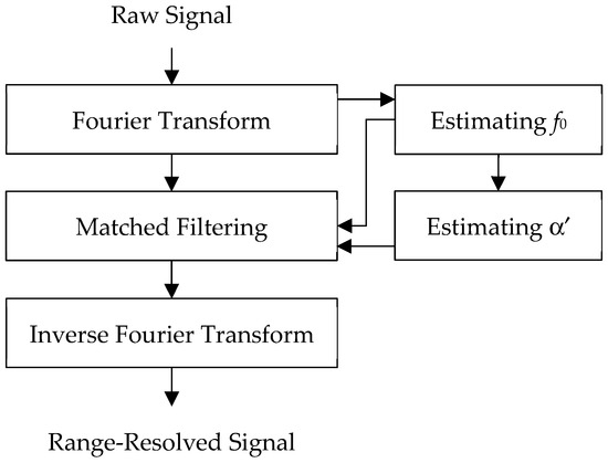
Figure 1.
Compensation of high-speed motion.
3. Simulation of ISAR Signals Under High-Speed Motion
In order to show the rationality of our theoretical analysis and the effectiveness of our compensation method, a scheme is presented to simulate the received signal under the high-speed motion of the target or the platform. This scheme assumes that the target and the platform move continuously with time and reflects the effects of the high-speed motion on the received signal accurately.
Figure 2 shows the geometry in the simulation. The radar moves along the dashed trajectory with velocities vr,x, vr,y, and vr,z in the x-axis, y-axis, and z-axis, respectively, and reaches the origin at time 0. The target moves with velocity vt,x in the x-axis.
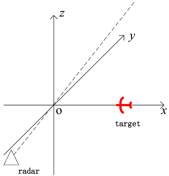
Figure 2.
Geometric relationship between platform and target in simulation.
The received signal is simulated echo by echo. Each echo is simulated by adding the pulses from all the scatterers when a chirp is transmitted. When a chirp is transmitted, the pulse from a scatterer is simulated in the following steps.
First, determine the indexes of samples where this pulse exists. This can be achieved once the start time and the end time of this pulse are found. Assume that t1 is the start time of the transmitted chirp, and this scatterer is located at position (xt, yt, zt) at time 0. Then, when the start edge of the chirp propagates from the radar to this scatterer, its delay τ1 can be found from
Here, the first equation is the motion equation of the start edge of the chirp when it propagates in a spherical wave, and other equations are the motion equations of this scatterer. The substitution of other equations into the first equation yields
where
The solution to this equation is
Assume that t2 is the time when the start edge of the chirp reaches the scatterer, that is, t1 + τ1. Then, when the start edge of the chirp propagates from this scatterer back to the radar, its delay τ2 can be found from
Here, the first equation is the motion equation of the start edge of the chirp when it propagates in a spherical wave, and other equations are the motion equations of the radar. The substitution of other equations into the first equation yields
where
The solution to this equation is
Next, the start time of this pulse can be found, that is, t2 + τ2. The end time of this pulse can be found similarly. Once the start time and the end time of this pulse are found, one can determine which indexes this pulse exists in in the echo.
Second, calculate the sample of this pulse at each index determined in the first step. Assume that a sample of the transmitted chirp is converted into the sample of this pulse at an index. Then, the sample of this pulse at this index can be calculated from this sample of the transmitted chirp if only the time for this sample of the transmitted chirp is found. This sample of the chirp propagates from the radar to this scatterer and then from the scatterer back to the radar. Assume that t3 is the time when this sample of the chirp returns to the radar. Then, when this sample of the chirp propagates from this scatterer back to the radar, its delay τ3 can be found from
Here, the first equation is the motion equation of this sample of the chirp when it propagates in a spherical wave, and other equations are the motion equations of the radar. The substitution of other equations into the first equation yields
where
The solution to this equation is
Assume that t4 is the time when this sample of the chirp reaches the scatterer, that is, t3 − τ3. Then, when this sample of the chirp propagates from the radar to this scatterer, its delay τ4 can be found from
Here, the first equation is the motion equation of this sample of the chirp when it propagates in a spherical wave, and other equations are the motion equations of this scatterer. The substitution of other equations into the first equation yields
where
The solution to this equation is
Next, the time for this sample of the transmitted chirp can be found, that is, t4 − τ4. So, the sample of this pulse at the given index can be calculated from this sample of the transmitted chirp.
4. Results and Discussion
A series of signals are simulated to show the rationality of the theoretical analysis and the effectiveness of the compensation method for the high-speed motion of the target or the radar in ISAR imaging. The geometry in simulation is shown in Figure 2. The radar transmits chirps with a carrier frequency of 10 GHz, a pulse width of 1 μs, a bandwidth of 250 MHz, and a pulse repetition frequency (PRF) of 500 Hz. The sampling frequency is 300 MHz. The target is an aircraft with a length of 15 m and a width of 9 m. Its components are simulated using lines, each consisting of discrete points. The aircraft flies at a speed of 200 m/s in the negative x-axis.
After acquiring a signal through simulation, the range-Doppler algorithm is used for ISAR imaging. First, a matched filter is used for range resolving. A Hamming window is used to suppress sidelobes in the matched filtering. Then, the global method [9,10] is used to carry out range alignment, and the sharpest-image method [18,19,20] is used to carry out phase adjustment. Finally, the Fourier transform is used for azimuth resolving. Figure 3 shows the overall processing flowchart.
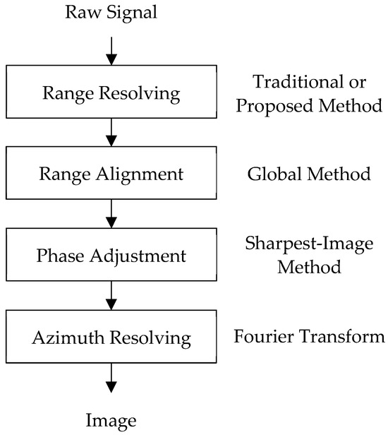
Figure 3.
Overall processing flowchart.
Each image has 512 × 512 pixels originally. In such an image, the target is too small to see clearly. For a clear view, the central 64 × 64 pixels of each image are taken and enlarged to show. In addition, the grayscales of each image are reversed in order that weak details can be seen more clearly. Thus, in each image, weak scatterers have high grayscales, and strong scatterers have low grayscales.
In the first case, the radar moves at velocities 3 km/s, 3 km/s, and 3 km/s in the x-axis, the y-axis, and the z-axis, respectively. Figure 4a shows the image when the signal is simulated under the “stop-and-go” assumption. This image is ideal but unreal because the signal is simulated under the “stop-and-go” assumption and contains no effects of the high-speed motion. Figure 4b shows the image when the signal is accurately simulated. This image is real because the signal is accurately simulated and thus contains the effects of the high-speed motion. However, as we see, this image is almost the same as the image in Figure 4a. This means that the effects of the high-speed motion are ignorable. Figure 4c shows the image when the signal is accurately simulated but the compensation of the high-speed motion is applied. Since the effects of the high-speed motion are imperceptible, the effectiveness of the compensation is imperceptible.
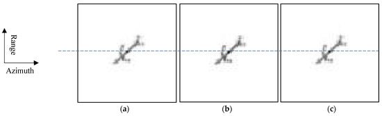
Figure 4.
Images when the radar moves at velocities 3 km/s, 3 km/s, and 3 km/s in the x-axis, the y-axis, and the z-axis, respectively. (a) Image under “stop-and-go” assumption (ideal but unreal); (b) image with accurate simulation (the effects of the high-speed motion are imperceptible); (c) and image with accurate simulation and high-speed compensation (the effectiveness of the compensation is imperceptible).
In the second case, the radar moves at velocities 20 km/s, 20 km/s, and 20 km/s in the x-axis, the y-axis, and the z-axis, respectively. Figure 5a shows the image when the signal is simulated under the “stop-and-go” assumption. The image is ideal but unreal because the signal is simulated under the “stop-and-go” assumption and contains no effects of the high-speed motion. Figure 5b shows the image when the signal is accurately simulated. The image is real because the signal is accurately simulated and thus contains the effects of the high-speed motion. It can be seen that this image has a shift in range, although its blurring in range is ignorable. Figure 5c shows the image when the signal is accurately simulated but the compensation of high-speed motion is applied. This compensation removes the shift of the image in range approximately, although its improvement of the focus quality of the image is imperceptible.
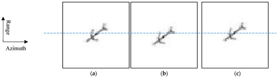
Figure 5.
Images when the radar moves at velocities 20 km/s, 20 km/s, and 20 km/s in the x-axis, the y-axis, and the z-axis, respectively. (a) Image under “stop-and-go” assumption (ideal but unreal); (b) image with accurate simulation (its shift in range can be seen although its blurring in range is imperceptible); and (c) image with accurate simulation and high-speed compensation (the compensation removes the shift in range approximately, although its improvement of the focus quality is imperceptible).
In the third case, the radar moves at velocities 50 km/s, 50 km/s, and 50 km/s in the x-axis, the y-axis, and the z-axis, respectively. Figure 6a shows the image when the signal is simulated under the “stop-and-go” assumption. The image is ideal but unreal because the signal is simulated under the “stop-and-go” assumption and contains no effects of the high-speed motion. Figure 6b shows the image when the signal is accurately simulated. The image is real because the signal is accurately simulated and thus contains the effects of the high-speed motion. It can be seen that this image has a significant shift in range, but its blurring in range is still ignorable. Figure 6c shows the image when the signal is accurately simulated but the compensation of high-speed motion is applied. This compensation removes the shift of the image in range, but its improvement of the focus quality of the image is still imperceptible.
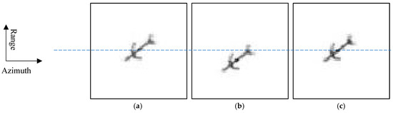
Figure 6.
Images when the radar moves at velocities 50 km/s, 50 km/s, and 50 km/s in the x-axis, the y-axis, and the z-axis, respectively. (a) Image under “stop-and-go” assumption (ideal but unreal); (b) image with accurate simulation (its shift in range is significant although its blurring in range is imperceptible); and (c) image with accurate simulation and high-speed compensation (the compensation removes its shift in range approximately, although its improvement of the focus quality is imperceptible).
Table 1 shows the range indexes of the strongest scatterer, which is located at the center of the target, in three schemes when the radar moves in different velocities. The theoretical shift in range is found according to Equation (16). It can be seen that the shift of the target in range can be clearly observed when the velocities of the radar in the x-axis, the y-axis, and the z-axis attain 4 km/s or higher, and it increases when the velocities of the radar in the x-axis, the y-axis, and the z-axis increase. It can also be seen that the compensation of high-speed motion removes the shift of the target in range.

Table 1.
Range indexes of strongest scatterer in different cases.
Entropy can be used to measure the focus quality of an image. Smaller entropy means better focus quality. Let g (m, n), where 0 ≤ m ≤ M − 1 and 0 ≤ n ≤ N − 1, be the complex image. The entropy of the image is defined as
Table 2 shows the entropies of the images in three schemes when the radar moves in different velocities. It can be seen that the entropy of the image steadily grows, that is, the focus quality of the image steadily degrades, when the velocities of the radar in the x-axis, the y-axis, and the z-axis attain 20 km/s or higher. In these cases, the compensation of high-speed motion decreases the entropy of the image and thus improves the focus quality of the image.
Table 2.
Entropies of images in different cases.
5. Conclusions
Deep research is carried out on the effects and the compensation of the high-speed motion of the target or the radar in ISAR imaging. Theoretical analysis shows that when a chirp is transmitted, the echo from a scatterer can be approximated as a chirp with its central frequency and chirp rate changed, which results in the shift and the blurring of the scatterer in range. As an important contribution, a method is presented to estimate the central frequency and the chirp rate, which are used to adjust the central frequency and the chirp rate of the matched filter. In this method, the central frequency is estimated to maximize the normalized correlation of the amplitude spectrum and its nominal form, and the chirp rate is derived from the central frequency. Moreover, to show the rationality of the theoretical analysis and the effectiveness of the compensation method, a scheme is presented to simulate the received signal under the high-speed motion of the target or the radar. This scheme assumes that the target and the radar move continuously with time and reflects the effects of the high-speed motion on the received signal accurately.
The motion of the target and the radar can be decomposed into the translation between the target and the radar and the rotation of the target. Our method can compensate the effects caused by the linear translation only. When the nonlinear translation and the rotation are also considered, the echoes from different scatterers will have different signal modes and thus need different matched filters for range resolving. Such effects cannot be compensated for by our method or other existing methods. Fortunately, generally, the effects of the nonlinear translation and the rotation are much smaller than the effects of the linear translation and thus can be neglected.
Author Contributions
Conceptualization, Z.W. and J.W.; methodology, Z.W. and J.W.; software, Z.W. and J.W.; validation, Z.W. and J.W.; formal analysis, Z.W. and J.W.; investigation, Z.W. and J.W.; data curation, J.W.; writing—original draft preparation, Z.W. and J.W.; writing—review and editing, Z.W. and J.W.; visualization, Z.W. and J.W.; supervision, J.W.; project administration, J.W.; and funding acquisition, J.W. All authors have read and agreed to the published version of the manuscript.
Funding
This work was supported by the National Natural Science Foundation of China (U2031127) and the Shanghai Academy of Spaceflight Technology Foundation (USCAST2022-30).
Data Availability Statement
Data are contained within the article.
Conflicts of Interest
The authors declare no conflicts of interest.
References
- Ausherman, D.A.; Kozma, A.; Walker, J.L.; Jones, H.M. Development in radar imaging. IEEE Trans. Aerosp. Electron. Syst. 1984, 20, 363–400. [Google Scholar] [CrossRef]
- Yang, S.; Li, S.; Fan, H.; Liu, Y. High-resolution ISAR imaging of maneuvering targets based on azimuth adaptive partitioning and compensation function estimation. IEEE Trans. Geosci. Remote Sens. 2023, 61, 5222115. [Google Scholar] [CrossRef]
- Li, H.; Li, X.; Xu, Z.; Jin, X.; Gao, J.; Su, F. An end-to-end multidomain interaction deep unrolling network based on block-aware optimization model for ISAR multitarget separation. IEEE Trans. Geosci. Remote Sens. 2025, 63, 5104813. [Google Scholar] [CrossRef]
- Zhang, L.; Qiao, Z.; Xing, M.; Sheng, J.; Guo, R.; Bao, Z. High-resolution ISAR imaging by exploiting sparse apertures. IEEE Trans. Antennas Propag. 2012, 60, 997–1008. [Google Scholar] [CrossRef]
- Zhang, S.; Liu, Y.; Li, X.; Bi, G. Joint sparse aperture ISAR autofocusing and scaling via modified Newton method-based variational Bayesian inference. IEEE Trans. Geosci. Remote Sens. 2019, 57, 4857–4869. [Google Scholar] [CrossRef]
- Zhang, Y.; Bai, X.; Liu, S.; Zhou, F. Joint translational motion compensation and high-resolution ISAR imaging based on sparse Bayesian learning. IEEE Trans. Comput. Imag. 2025, 11, 1115–1127. [Google Scholar] [CrossRef]
- Gao, J.; Deng, B.; Qin, Y.; Wang, H.; Li, X. Enhanced radar imaging using a complex-valued convolutional neural network. IEEE Geosci. Remote Sens. Lett. 2019, 16, 35–39. [Google Scholar] [CrossRef]
- Hu, C.; Wang, L.; Li, Z.; Zhu, D. Inverse synthetic aperture radar imaging using a fully convolutional neural network. IEEE Geosci. Remote Sens. Lett. 2020, 17, 1203–1207. [Google Scholar] [CrossRef]
- Wang, Y.; Bai, X.; Zhou, F. Robust joint translational motion compensation and high-resolution ISAR imaging based on TMC-EADMM-Net. IEEE Trans. Aerosp. Electron. Syst. 2025, 61, 1–15. [Google Scholar] [CrossRef]
- Wehner, D.R. High Resolution Radar, 2nd ed.; Artech House: Norwood, MA, USA, 1994. [Google Scholar]
- Prickett, M.J.; Chen, C.C. Principle of inverse synthetic aperture radar (ISAR) imaging. In Proceedings of the EASCON 1980; Electronics and Aerospace Systems Conference, Arlington, VA, USA, 1 October 1980; pp. 340–345. [Google Scholar]
- Pastina, D.; Farina, A.; Gunning, J.; Lombardo, P. Two-dimensional super-resolution spectral analysis applied to SAR images. IEE Proc. Radar Sonar Navig. 1998, 145, 281–290. [Google Scholar] [CrossRef]
- Chen, V.C. Joint time-frequency transform for radar range-Doppler imaging. IEEE Trans. Aerosp. Electron. Syst. 1998, 34, 486–499. [Google Scholar] [CrossRef]
- Chen, C.C.; Andrews, H.C. Target-motion-induced radar imaging. IEEE Trans. Aerosp. Electron. Syst. 1980, 16, 2–14. [Google Scholar] [CrossRef]
- Sauer, T.; Schroth, A. Robust range alignment algorithm via Hough transform in an ISAR imaging system. IEEE Trans. Aerosp. Electron. Syst. 1995, 31, 1173–1177. [Google Scholar] [CrossRef]
- Li, X.; Kozma; Liu, G.; Ni, J. Autofocusing of ISAR images based on entropy minimization. IEEE Trans. Aerosp. Electron. Syst. 1999, 35, 1240–1251. [Google Scholar]
- Wang, J.; Kasilingam, D. Global range alignment for ISAR. IEEE Trans. Aerosp. Electron. Syst. 2003, 39, 351–357. [Google Scholar] [CrossRef]
- Wang, J.; Liu, X. Improved global range alignment for ISAR. IEEE Trans. Aerosp. Electron. Syst. 2007, 43, 12–17. [Google Scholar] [CrossRef]
- Eichel, P.H.; Ghiglia, D.C.; Jakowatz, C.V. Speckle processing method for synthetic aperture radar phase correction. Opt. Lett. 1989, 14, 1–5. [Google Scholar] [CrossRef]
- Wahl, D.E.; Eichel, P.H.; Ghiglia, D.C.; Jakowatz, C.V. Phase gradient autofocus—A robust tool for high resolution SAR phase correction. IEEE Trans. Aerosp. Electron. Syst. 1994, 30, 827–835. [Google Scholar] [CrossRef]
- Barbarossa, S.; Farina, A. A novel procedure for detecting and focusing moving objects with SAR based on the Wigner-Ville distribution. In Proceedings of the IEEE International Radar Conference, Arlington, VA, USA, 7–10 May 1990. [Google Scholar]
- Berizzi, F.; Cosini, G. Autofocusing of inverse synthetic radar images using contrast optimization. IEEE Trans. Aerosp. Electron. Syst. 1996, 32, 1191–1197. [Google Scholar] [CrossRef]
- Bocker, R.P.; Henderson, T.B.; Jones, S.A.; Frieden, B.R. A new inverse synthetic aperture radar algorithm for translational motion compensation. In Stochastic and Neural Methods in Signal Processing, Image Processing, and Computer Vision; SPIE: Bellingham, WA, USA, 1991; Volume 1569, pp. 298–310. [Google Scholar]
- Fienup, J.R. Synthetic-aperture radar autofocus by maximizing sharpness. Opt. Lett. 2000, 25, 221–223. [Google Scholar] [CrossRef]
- Fienup, J.R.; Miller, J.J. Aberration correction by maximizing generalized sharpness metrics. J. Opt. Soc. Am. A 2003, 20, 609–620. [Google Scholar] [CrossRef] [PubMed]
- Wang, J.; Liu, X.; Zhou, Z. Minimum-entropy phase adjustment for ISAR. IEE Proc. Radar Sonar Navig. 2004, 151, 203–209. [Google Scholar] [CrossRef]
- Wang, J.; Liu, X. Measurement of sharpness and its application in ISAR imaging. IEEE Trans. Geosci. Remote Sens. 2013, 51, 4885–4892. [Google Scholar] [CrossRef]
- Wang, J. Convergence of the fixed-point algorithm in ISAR imaging. Remote Sens. Lett. 2023, 14, 993–1001. [Google Scholar] [CrossRef]
- Zeng, T.; Wang, R.; Li, F. SAR image autofocus utilizing minimum-entropy criterion. IEEE Geosci. Remote Sens. Lett. 2013, 10, 1552–1556. [Google Scholar] [CrossRef]
- Min, C.; Fu, Y.; Jiang, W.; Li, X.; Zhuang, Z. High resolution range profile imaging of high speed moving targets based on fractional Fourier transform. In Proceedings of the MIPPR 2007: Automatic Target Recognition and Image Analysis; and Multispectral Image Acquisition, Wuhan, China, 15–17 November 2007. [Google Scholar]
- Zhang, S.; Sun, S.; Zhang, W.; Zong, Z.; Yeo, T. High-resolution bistatic ISAR image formation for high-speed and complex-motion targets. IEEE J. Sel. Top. Appl. Earth Obs. Remote Sens. 2015, 8, 3520–3531. [Google Scholar] [CrossRef]
- Tian, B.; Chen, Z.; Xu, S.; Liu, Y. ISAR imaging compensation of high speed targets based on integrated cubic phase function. In Proceedings of the 8th Symposium on Multispectral Image Processing and Pattern Recognition (MIPPR)—Multispectral Image Acquisition, Processing, and Analysis, Wuhan, China, 26–27 November 2013. [Google Scholar]
- Guo, B.; Li, Z.; Xiao, Y.; Shi, L.; Han, N.; Zhu, X. ISAR Speed Compensation Algorithm for High-speed Moving Target Based on Simulate Anneal. In Proceedings of the 2019 IEEE 19th International Conference on Communication Technology (ICCT), Xi’an, China, 16–19 November 2019. [Google Scholar]
- Sheng, J.; Fu, C.; Wang, H.; Liu, Y. High Speed Motion Compensation for Terahertz ISAR Imaging. In Proceedings of the 2017 International Applied Computational Electromagnetics Society Symposium (ACES), Suzhou, China, 1–4 August 2017. [Google Scholar]
- Li, J.; Zhang, Y.; Yin, C.; Xu, C.; Li, P.; He, J. A Novel Joint Motion Compensation Algorithm for ISAR Imaging Based on Entropy Minimization. Sensors 2024, 13, 4332. [Google Scholar] [CrossRef]
- Bamler, R. Doppler frequency estimation and the Cramer-Rao bound. IEEE Trans. Geosci. Remote Sens. 1991, 29, 385–390. [Google Scholar] [CrossRef]
Disclaimer/Publisher’s Note: The statements, opinions and data contained in all publications are solely those of the individual author(s) and contributor(s) and not of MDPI and/or the editor(s). MDPI and/or the editor(s) disclaim responsibility for any injury to people or property resulting from any ideas, methods, instructions or products referred to in the content. |
© 2025 by the authors. Licensee MDPI, Basel, Switzerland. This article is an open access article distributed under the terms and conditions of the Creative Commons Attribution (CC BY) license (https://creativecommons.org/licenses/by/4.0/).