Article

An Adaptive PID Controller for Longitudinal Velocity and Yaw Rate Tracking of Autonomous Mobility Based on RLS with Multiple Constraints

1
School of Automotive Engineering, Kyungpook National University, Sangju 37311, Republic of Korea
2
School of ICT, Robotics & Mechanical Engineering, Hankyong National University, Anseong 17579, Republic of Korea
*
Author to whom correspondence should be addressed.
Electronics 2025, 14(20), 4111; https://doi.org/10.3390/electronics14204111
Submission received: 14 September 2025 / Revised: 17 October 2025 / Accepted: 17 October 2025 / Published: 20 October 2025
(This article belongs to the Special Issue Automated Driving Systems: Latest Advances and Prospects)

Abstract

Recently, various forms and purposes of autonomous mobility have been widely developed and commercialized. To control the various iterations of shaped and purposeful mobility, control technology that can adapt to the dynamic characteristics of the mobility and environmental changes is essential. This study presents an adaptive proportional–integral–derivative (PID) controller for longitudinal velocity and yaw rate tracking in autonomous mobility, addressing the aforementioned issue. To design the adaptive PID controller, error dynamics have been designed using error and control input with two coefficients. It is designed that the two coefficients are estimated in real time by recursive least squares with multiple constraints and forgetting factors. The estimated coefficients are used to compute PI gains based on the Lyapunov direct method with constant derivative gain. Multiple constraints, such as value and rate limits, have been incorporated into the RLS algorithm to enhance the control stability. The performance evaluation is conducted through the co-simulation of MATLAB/Simulink and CarMaker under integrated control scenarios, such as longitudinal velocity and yaw rate tracking, for mobility.

1. Introduction

Autonomous driving has rapidly advanced in recent years, driven by advances in computing power and the proliferation of sensor and ADAS technologies. Research has shown that autonomous driving systems generally have a lower accident rate than human-driven vehicles, and the risk is relatively low in straight-line and regular driving situations. However, research has also shown that autonomous vehicles are no less dangerous than human drivers during dawn and dusk or cornering conditions [1]. Research continues to ensure the comfort, fuel efficiency, and, most importantly, driving safety of autonomous vehicles.
Fundamentally, the key components of autonomous driving performance can be categorized into perception, localization, path planning, and path tracking [2,3]. Perception and localization rely heavily on sensor performance, such as radar, cameras, and lidar, and thus active research is being conducted to improve sensor levels. In contrast, path-planning-based path-tracking control directly influences the vehicle’s actual behavior. This crucial function is closely linked to the vehicle’s physical dynamics.
Path-tracking control can be defined as a function that comprehensively controls the vehicle’s position along a predetermined local path, considering factors such as environmental awareness, the global map, and the vehicle’s position, while simultaneously considering stability, precision, and ride comfort. In short, it performs control to minimize errors so that the vehicle follows a predetermined path in both the longitudinal and lateral directions.
Much research has been conducted on path tracking, with the Pure Pursuit model [4] and the Stanley model [5], introduced at the DARPA Urban Challenge, being representative early models. The Pure Pursuit model is a path-tracking algorithm that uses only the vehicle’s dynamic equations and the geometry of a reference path. It assumes the vehicle to be a bicycle or an Ackermann model and uses the center of the rear wheel as a reference point. However, it suffers from reduced control accuracy at large curvatures. Unlike the Pure Pursuit model, which is based on the center of the rear wheel, the Stanley model uses the front axle as a reference point. It improves path-tracking precision by calculating the steering angle and considering the position error to the target point and the vehicle’s heading error. Because these two models are based on a kinematic model of the vehicle, they are simple and easy to implement, and have been widely applied. However, they have limitations in ensuring autonomous vehicles’ driving stability and robust control performance. Consequently, active research has been conducted on feedback controller design and stability/robustness verification, which considers vehicle dynamics, nonlinearity, and uncertainty.
One of the main research trends is an increasing focus on path-tracking performance, considering the limits of handling performance at high speeds. Funke et al. [6] proposed an integrated MPC that simultaneously considers the potentially conflicting control objectives of collision avoidance, path following, and vehicle stabilization. In a real-world rear-wheel-drive electric vehicle test, the proposed controller successfully utilized the vehicle performance to avoid and stabilize the vehicle, even when obstacles appeared or suddenly appeared in the middle of a curve. However, the discussion of vehicle uncertainty and real-time constraints is only suggestive.
He, Z. et al. [7] proposed a hierarchical controller for lateral path-following control of autonomous vehicles. The upper-level controller generates an optimal steering angle to ensure vehicle stability by considering vehicle dynamics and tire slip angle constraints, and the lower-level controller applies an RBFNN-based adaptive PID controller. They demonstrated that vehicle stability is significantly improved while maintaining the path-following performance by adaptively adjusting PID control parameters, by identifying nonlinearities and time variations in the steering system online.
Menhour et al. [8] proposed a model-free control technique for longitudinal and lateral vehicle control and verified its performance through experiments and simulations. They proposed a technique for identifying state variables in real time through algebraic estimation, which estimates system nonlinearities and uncertainties, including vehicle behavior and disturbances, and generates intelligent PID-type control signals based on these state variables.
Lee, K. et al. [9] proposed an LQG controller that automatically provides the optimal path-following performance without separate tuning, unlike traditional Stanley and Pure-Pursuit controllers, adaptively adjusting the Q-matrix of the LQG controller to changes in vehicle speed and driving conditions, thereby maintaining consistent path-following characteristics without vibration under various vehicle conditions.
Ahn, J. et al. [10] proposed a new method for adjusting the look-ahead point by considering the geometric relationship between the vehicle and the path to address the performance limitations of the Pure Pursuit method, a widely used path-following method. Gong et al. [11] applied imitation learning to initial policy learning to solve existing data-driven problems such as data quality issues and learning costs, and introduced the concept of “life-long learning” to safely update policies and improve the performance by utilizing operation data gradually accumulated online.
Marino et al. [12] designed a standard PID control for two outputs (lateral offset and yaw rate) and one input to ensure system robustness. Their architecture, consisting of two independent control loops, demonstrated theoretical robustness and a superior performance compared to model predictive control methods, especially in scenarios involving speed variations and uncertain vehicle parameters. Ma, Y. et al. [13] proposed a control strategy that improved the path-following performance and yaw stability of autonomous vehicles by applying a port-Hamiltonian model and an energy shaping-based IDA-PBC (interconnection and damping assignment passivity-based Control) technique.
Liang, Y. et al. [14] simulated path following and dynamic stability integration in 4WID/4WIS autonomous vehicles through LMI-based kinematic control, a prediction-based cooperative mechanism, and hierarchical torque and force distribution. This paper’s prediction-based yaw rate control is based on simple extrapolation (polynomial extrapolation) and threshold values at fixed time intervals. However, it was pointed out that sensor noise, signal delay, actuator nonlinearity, and delay characteristics can be significant issues in actual hardware. Wang, X. et al. [15] proposed an algorithm that dynamically controls the steering angle and speed of a vehicle by applying fuzzy logic. They applied multiple look-ahead distances to reduce the noise impact of path estimation and achieved stable lateral control under various driving conditions (forward and backward, various curvature paths, etc.). However, designing fuzzy rules and membership functions requires a lot of time and effort, which can be a burden when applied to vehicles.
Since then, various studies have applied techniques, including PID control, to path and trajectory stabilization problems. Various motion-planning algorithms that reflect the inherent nonholonomic constraints of vehicles and feedback control techniques that satisfy them in real time have been developed. In particular, model predictive control (MPC), which considers a vehicle dynamics model, has been actively applied recently [16].
Yao, Q. et al. [17] proposed an MPC controller that compensates for longitudinal velocity changes within the prediction interval, thereby improving the prediction error caused by the constant velocity assumption of conventional MPC. Polynomial approximation and linearization techniques were utilized for this purpose. Lin F et al. [18] proposed adaptive model predictive control (AMPC), which can adapt to external environmental changes such as vehicle speed and road surface conditions. To achieve this, a real-time recursive least square (RLS)-based estimator was designed to estimate the tire cornering stiffness and road friction coefficient in real time, and the estimated vehicle dynamics model and control constraints were dynamically updated. K Zhu et al. [19] proposed a new recursive least squares identification algorithm with variable-direction forgetting to enhance the parameter estimation performance under non-persistent excitation. P Sarhadi et al. [20] developed an adaptive control algorithm with a dynamic anti-windup compensator for an autonomous underwater vehicle. In the study, a modern AW technique was employed to cope with the saturation problem. O Garpinger et al. [21] developed a new software-based method for optimal PID and filter design with robustness and noise sensitivity constraints. The authors visualized the performance, robustness, and noise sensitivity trade-offs for a representable process type.
Chu, D et al. [22] proposed a path-planning system utilizing an improved artificial potential field and a feedback control structure combining model predictive control (MPC) and PID control. This approach addressed the model simplification issues of conventional MPC-based control (especially the increased accumulated error on curves), the tuning burden, and the lack of scalability of pure PID controllers.
Using a model-free approach, Liu et al. [23] applied artificial flow guidance (AFG) to a 4WS vehicle. This method simultaneously tracks the center points of the front and rear axles of the vehicle using a pre-generated two-dimensional velocity field, ensuring path following and driving stability. It utilizes only position and velocity information as inputs, eliminating the need for complex vehicle models or parameter tuning, resulting in lightweight and easy real-time implementation.
Tork et al. [24] proposed an adaptive neural network-based lateral–longitudinal control system. To address vehicle dynamic nonlinearity and uncertainty issues, they used interval type-2 fuzzy sets (IT2FS) as an activation function, improving the simultaneous lateral and longitudinal control performance, a key area overlooked in previous studies.
Considering the practicality of PID controllers, numerous studies have been conducted to improve their stability and performance. The first approach is the integration of MPC with conventional nonlinear control, and the second is the integration with learning based models. Shan, Y. et al. [25] emphasized the importance of balancing safety (tracking accuracy) and ride comfort (passenger experience). They proposed a hybrid steering control method (combining Pure Pursuit and PID controllers), incorporating a reinforcement learning model and a rough-to-fine velocity adaptation method. The hybrid structure (PP_PID) combining Pure Pursuit geometric controllers and PID controllers was designed to automatically adjust to changing conditions by applying reinforcement learning (Proximal Policy Optimization, PPO).
Tang, M. et al. [26] proposed a novel prediction-based path-following control method that combines a visual prediction model with multi-process control (MPC) and includes a PID stabilization controller to address high nonlinearity and longitudinal–lateral coupling issues in tracking control. Simulation results confirmed that the proposed method optimizes the vehicle tracking performance and improves accuracy under various road conditions and high-speed driving environments.
Zeng, D. et al. [27] compared various lateral control techniques, such as LQR, MPC, and NISMC, based on a 3-DOF vehicle model. In lateral control, MPC showed the best performance in the simulation results, and especially on low-adhesion roads, it recorded the highest overall performance score, demonstrating an excellent tracking performance, resistance to interference, and robustness. Although LQR has a slightly lower overall performance than MPC, it offers advantages in real-time processing and computational complexity. It effectively maintains control stability, but can result in excessive front wheel steering angle output. NISMC (nonlinear integral sliding mode control) has an excellent accuracy and response time under optimal and typical road conditions. However, its control effectiveness decreases significantly when road conditions become severe or curvature changes significantly, recording the lowest overall performance score on low-adhesion roads. PID was recommended as the preferred choice for a longitudinal speed tracking controller in longitudinal control, as it responds quickly and accurately to the reference speed in step speed-tracking tests. At the same time, MPC was found to have limitations such as a jittering effect during speed changes due to parameter constraints and other issues, slow braking response, higher requirements for system modeling accuracy, and higher computational complexity.
Some research has also been conducted to improve vehicle path-tracking control by improving the PID controller. Simorgh et al. [28] proposed an adaptive PID (proportional–integral–derivative) control system for longitudinal speed control of autonomous vehicles. To ensure that the vehicle speed accurately tracks the target speed under realistic road conditions and disturbances such as air resistance, the PID parameters were adjusted using a robust update rule and σ-modification technique to compensate for disturbances and nonlinearities. The performance was verified through CarSim analysis.
Previous research suggests that vehicle path-tracking control has evolved from a simplified kinematic model-based approach to model predictive control (MPC), which considers vehicle dynamics and performance indicators. Simultaneously, model-free and learning-based approaches are also actively being studied. However, MPC still suffers from limitations in robustness due to the computational burden, vehicle model uncertainty, and external environmental uncertainty.
Consequently, this study proposes a self-tuning PID control approach, rather than a model-based approach, for application to autonomous vehicle path-tracking control. PID control can guarantee system robustness by optimizing gains according to system conditions, and real-time performance can be achieved relatively easily through model-based methods. Furthermore, because it relies less on system modeling, it can be applied to any vehicle model. However, due to its dependence on system feedback states, a gain-tuning method is required to ensure both speed and stability.
The area of self-adaptive PID control, which this study explores, is still actively being studied in various industrial applications, including processes, robotics, and mechanical systems. Early research [29] focused on proving global stability. Using a variable-structure PID, Jafarov et al. [30] demonstrated the utility of a PID sliding-mode controller that does not require equivalent control terms requiring dynamic knowledge. Future research will expand to include intelligent gain-tuning techniques that ensure system control stability simultaneously.
Toru Yamamoto [31] proposed a novel PID controller design method using data-driven modeling, addressing the high learning costs of existing neural network and genetic algorithm-based methods. The effectiveness and practicality of the proposed method were verified through simulation examples and experiments on a pilot-scale temperature control system. Li, X. H. [32] proposed an optimal PID controller based on Lyapunov theory. They transformed the optimal control problem into a nonlinear constrained optimization (NLCO) problem and solved it. Their simulation results demonstrated that this approach provided a superior control performance and stability compared to existing empirical tuning methods.
Norlund, F. [33] proposed a novel configuration where an MPC controller is designed based on the PID closed loop to enable a smooth transition between unconstrained PID operation and MPC-dominated control. The proposed controller was demonstrated using a relevant process industrial application. Saat, S. [34] developed an enhanced safe experimentation dynamics algorithm to address the issue that control performance can be limited by the fixed probability coefficient. The algorithm was validated using simulations on multi-input, multi-output systems, with a focus on tracking performance and computational efficiency.
In this study, we address the potential performance degradation of model-based adaptive controllers due to model uncertainty and the need for a disturbance estimator to overcome this. Applying a disturbance estimator, however, increases computational complexity and, if model uncertainty is relatively high, reduces the utility of the estimated disturbance. Therefore, we propose a stable, mathematical model and system parameter-independent adaptive proportional–integral–derivative control algorithm that can be applied universally to diverse mechanical and electrical systems including mobility.
The remainder of this paper is organized as follows. Section 2 describes an adaptive PID control algorithm based on multiple constraints, and Section 3 provides some performance evaluation results with its analysis. Section 4 provides a discussion, concluding remarks, and limitation analysis with future works.

2. Adaptive PID Controller Based on RLS with Multiple Constraints

Figure 1 shows a block diagram of this study’s proposed adaptive PID control algorithm with a gain self-tuning algorithm.
The algorithm consists of two blocks, such as a PID control input and gain self-tuning block. In the gain self-tuning block, proportional and integral gains are self-tuned based on the estimated coefficients and control error. The self-tuned proportional and integral gains compute the control input in the PID control input block. In this study, the derivative gain is set to a constant value, and it is assumed that the derivative gain can be determined reasonably either empirically or theoretically.

2.1. Adaptive PID Controller Design with Gain-Self Tuning

The error dynamics for PI gain self-tuning are given by Equation (1). Here, a, b, and e are coefficients estimated online by RLS and control error, respectively.
e ˙ = a e + u k d e ˙ + b 0 t e d t ,
The error dynamic equation is designed so that the derivative and integral action terms influence the dynamics as a disturbance of the dynamics. The design form in Equation (1) means PI gains update reasonably. It is designed so that the coefficients a and b are estimated in real time based on recursive least squares with multiple forgetting factors. Equation (1) can be rewritten as the following equation.
1 + k d e ˙ u = e 0 t e d t a b ,
Equations (3)–(5) are the output, regressor, and estimate, respectively. The output can be calculated using the derivative gain, the time derivative of error, and the total PID control input u. The regressor matrix ϕ consists of the control error and its integration. The estimate matrix θ consists of coefficients a and b used to design error dynamics.
y = 1 + k d e ˙ u ,
ϕ = e 0 t e d t T ,
θ = a b T ,
Based on the above Equations (3)–(5), the RLS algorithm has been designed with multiple forgetting factors for real-time estimation of coefficients. The following Equations (6)–(9) are the equations for gain, covariance, and estimate update [35].
y = ϕ T θ ,
L k = P k 1 ϕ k λ + ϕ k T P k 1 ϕ k 1 ,
θ k = θ k 1 + L k y ϕ k T θ k 1 ,
P k = I L k ϕ k T P k 1 / λ ,
L , P , and λ represent the update gain, covariance, and forgetting factor, respectively. It is designed that the above equations are computed for every sequence for real-time estimation of coefficients a and b. To evaluate the parameter identifiability based on a sensitivity analysis of the regressor matrix defined in Equation (4), the condition number has been analyzed theoretically with a pseudo inverse and Euclidean norm (2-norm). By using Equation (6), the condition number of the regressor matrix can be derived based on the Euclidean norm and pseudo inverse as in the following process.
θ 2 θ 2 ϕ 2 ϕ + 2 y 2 y 2 ,
C o n d ϕ T = ϕ 2 ϕ + 2 = e 0 t e d t T 2 e 0 t e d t T + 2 ,
C o n d ϕ = e 2 + 0 t e d t 2 e 2 + 0 t e d t 2 e 2 + 0 t e d t 2 = 1 ,
It is shown that the value of the condition number of the regressor matrix is always equal to one regardless of the control error and its integral term. In this study, the typical PID control input is used, shown as follows.
u = k p e + k i 0 t e d t + k d e ˙ ,
k p , k i , and k d are the proportional, integral, and derivative gains. It is assumed that the derivative gain can be determined reasonably, and the gain is set to be constant in this study. The self-tuning algorithm of the proportional and integral gains has been designed with the following integrated error value using weighting factor w.
s = e + w 0 t e d t ,
Based on the above-defined integrated error S, the cost function has been defined to design the self-tuning algorithm for proportional and derivative gains.
J = 1 2 s 2 ,
In this study, the Lyapunov direct method has been used to derive a self-tuning rule based on the defined cost function in Equation (15). The following equation is the time derivative of the defined cost function. The time derivative of the integrated error can be derived from the Equation (15), and it can be rewritten as follows.
J ˙ = s s ˙ = s e ˙ + w e ,
The asymptotic stability condition has been applied so the control error converges to zero asymptotically, and the following equation is the applied condition.
J ˙ = α J ,
α is the reduction rate for the cost function, and its value has been defined by a positive value. Based on the asymptotic stability condition, the time derivative of the cost function can be rewritten using the control error and its integration.
a + k p + w + a / 2 e = k i b α w / 2 0 t e d t ,
To meet the equality condition of the above Equation (18) for asymptotic stability, the following conditions in Equations (19) and (20) have been designed. The first condition in Equation (19) is that the equation in parentheses on the left term is defined as integrating the control error. The second condition in Equation (20) is that the equation in parentheses on the right-hand term is defined as the control error.
a + k p + w + α 2 = 0 t e d t ,
k i b α w 2 = e ,
From the defined conditions in Equations (19) and (20), the proportional and integration gains can be derived, and the derived gains are shown in Equations (21) and (22). Because the coefficients a and b are self-tuned by the RLS algorithm, and the control error and its integrated value are changed in real time, gains are self-tuned in real time.
k p = a ^ w α 2 + 0 t e d t ,
k i = b ^ α w 2 e ,

2.2. Multiple Constraints

Figure 2 shows the detailed block diagram of the gain self-tuning block in Figure 1; the block diagram consists of two blocks, such as RLS with forgetting and rate limiter blocks for a constrained RLS.
Here, a ^ and b ^ are estimated coefficients, respectively, and a ^ R L and b ^ R L are rate-limited estimated coefficients as constraints of the RLS algorithm. In the RLS with a forgetting block, coefficients a and b used for gain self-tuning are estimated based on the recursive least squares method with multiple forgetting. The change rate of the estimated coefficients is limited by the rate limiter block to avoid a sudden change in coefficients’ values. The rate limit value was determined empirically through an iterative tuning process. This study has applied two external conditions to the RLS algorithm as constraints to prevent the self-tuned gains from taking on negative values as follows.
k p = a ^ w α 2 + 0 t e d t 0 ,
k i = b ^ α w 2 e 0 ,
To ensure the stability of the RLS and control algorithms, determining the initial estimate value of the RLS algorithm is important. Therefore, the initial estimate values of the coefficients are determined based on the following inequality conditions.
k p , i n i t = a ^ i n i t w α 2 + 0 t e d t = η p 0 ,
k i , i n i t = b ^ i n i t α w 2 e = η i 0 ,
η p and η i are relatively small positive values that can make the initial gains ( k p , i n i t , k i , i n i t ) positive. Equations (27) and (28) are the initial coefficients ( a ^ i n i t , b ^ i n i t ) used for the RLS algorithm when the algorithm is activated with initial error and its integration.
a ^ i n i t = w a 2 + 0 t e d t η p ,
b ^ i n i t = α w 2 e η i ,
In this study, multiple constraints such as the rate limit of the estimates, as shown in Figure 2, and non-negative conditions of k p and k i in Equations (23) and (24) are implemented to the RLS algorithm for the real-time calculation process.
It is worth noting that while projection-based RLS methods [19] directly enforce constraints within the parameter update law, this study applies constraints externally (non-negativity in Equations (23) and (24) and rate limiter in Figure 2). This design choice offers several advantages: (i) implementation simplicity—each constraint can be applied independently without modifying the core RLS recursion (Equations (6)–(9)), (ii) flexibility—individual constraint thresholds can be adjusted without re-deriving projection operators, and (iii) computational efficiency—avoiding matrix projections reduces the real-time computational burden, which is critical for embedded automotive control units.
Unlike K Zhu et al. [19], who uses variable-direction forgetting to handle non-persistent excitation, our approach combines a forgetting coefficient with several constraints (non-negativity and rate limiters) to ensure a stable parameter evolution. Similar to the anti-windup compensator of P Sarhadi et al. [20], the rate limiter in our study prevents abrupt parameter changes that could destabilize the system. The noise sensitivity constraint of O Garpinger et al. [21] can be viewed as analogous to the rate limiter filtering out measurement noise. Our direct Lyapunov-based gain synthesis (Section 2.1) maps the estimated coefficients directly to the PI gain, enabling model-agnostic adaptation without process identification. The next subsection describes the stability analysis of the proposed adaptive PID control algorithm.

2.3. Stability Analysis with Persistency of Excitation

The stability analysis has been conducted based on a theoretical approach and Lyapunov’s direct method. The following is the stability proof of the proposed controller.
Assumption 1.
Let e be the tracking error and s = e + w e d t with w > 0 , as in Equations (12) and (13). The control input is Equation (11) with a fixed k D 0 . Coefficients θ = a b T estimated online by RLS with a forgetting factor and rate-limited to avoid abrupt changes (see Figure 2and “Rate limiter” block). The initialization and non-negativity constraints, as specified in Equations (20)–(25), are enforced.
  • Signal boundedness:  e ˙ used in Equations (3) and (13) is obtained via a causal differentiator and is bounded; the reference and measured states remain bounded over the operating region.
  • RLS boundedness:  P 0 0 , λ     0,1 ,  and the regressor  ϕ = e 0 t e d t T is bounded.
  • Gain constraints:  k P ( t ) ,     k I ( t )  computed by Equations (21) and (22) satisfy Equations (23)–(28) for all  t .
  • Excitation for identification: There exists T ,     μ 1 ,     μ 2 > 0 such that μ 1 I t t + T ϕ ( τ ) ϕ ( τ ) d τ μ 2 I (persistently exciting condition with a locally integrable function ϕ ( t ) ).
Lemma 1.
(RLS with forgetting—boundedness/convergence). Under RLS boundedness and the rate-limit/constraint implementation, the RLS estimate  θ ^ ( t ) and covariance  P ( t )  remain bounded for bounded  ϕ . If excitation for identification also holds and measurement noise is zero, then  θ ^ ( t ) θ  exponentially. With bounded noise, the parameter error is bounded and  P ( t )  remains positive definite. (RLS Equations (6)–(9); see also [35].) Here,  θ  denotes the unknown ground-truth parameter vector of the error dynamics, i.e.,  θ * = [ a * b * ] T  satisfying y = ϕ θ ;  θ ^  is its RLS estimate and  θ ~ = θ ^ θ  is the estimation error.
Theorem 1.
(Closed-loop control stability).
Consider the PI update laws Equations (21) and (22) obtained by enforcing J ˙ = α J with α > 0 (cf. Equations (15)–(18)). Under signal boundedness and gain constraints, in the ideal case where θ ^ = θ (no estimation error), the system satisfied J ( t ) = J ( 0 ) e α t and e ( t ) 0 exponentially. In the presence of estimation/measurement errors, there exists a class- K L bound such that
J ( t )     J ( 0 ) e α t + β ( sup 0 τ t ( θ ~ ( τ ) + ν ( τ ) ) ) ,
where θ ^ = θ ^ θ , and ν collects bounded perturbations from numerical differentiation and sensors. Thus, the closed loop is input-to-state stable with respect to ( θ ^ , ν ) ; if θ ^ 0 , e.g., excitation for identification holds and noise is negligible, then e ( t ) 0 exponentially. Based on Lemma 1, the equality of the error dynamics in Equation (1) is approximately valid in the real-time process, and the covariance in Equation (9) converges to near zero with the forgetting factor value near 1. For all j 0 and k j , the following equation is defined to investigate the effect of persistent excitation and forgetting.
H j , k i = j k ϕ ( i ) ϕ ( i ) ,
Based on Lemma 1 with forgetting factor value 1 and positive definite P 0 1 , for all k 1 , the covariance P k can be written as follows using Equations (7), (9), and (30). T in Equation (32) represents the sampling time for the discrete sequence of the control algorithm.
P k 1 = H 0 , k + P 0 1 ,
k T / T + 1 μ 1 I + P 0 1 P k 1 k T / T + 1 μ 2 I + P 0 1 ,
Therefore, the covariance P k converges to zero as k goes to infinity. With the Lemma and Theorem, the time derivative of the Lyapunov function in Equation (16) can be rewritten as follows using the error dynamics, definition of s in Equation (14), and estimates a ^ and b ^ .
J ˙ = s s ˙ = s e ˙ + w e = s a ^ e + u k d e ˙ + b ^ 0 t e d t + w e ,
The above equation can be rewritten as follows using the PID control input in Equation (13) with the self-tuned PI gains in Equations (21) and (22).
J ˙ = s a ^ e + k p e + k i 0 t e d t + k d e ˙ k d e ˙ + b ^ 0 t e d t + w e ,
J ˙ = s a ^ e + a ^ w α 2 + 0 t e d t e + b ^ α w 2 e 0 t e d t + b ^ 0 t e d t + w e ,
J ˙ = s α 2 e α w 2 0 t e d t ,
The above Equation (36) can be simplified as follows with the definition of s, and it can be shown that the time derivative the cost function J is asymptotically stable with positive α .
J ˙ = α 1 2 s e + w 0 t e d t = α 1 2 s 2 = α J ,
Based on the above stability analysis with persistency of excitation, it is shown that the s variable always goes to zero asymptotically. Also, when combining Lemma 1 with Theorem 1, the proposed adaptive PI law with constraints Equations (21)–(26) yields asymptotic tracking in the noise-free PE case and practical tracking (bounded error) under bounded disturbances. The following section describes the performance evaluation results using the co-simulation technique of MATLAB/Simulink(2019a) and CarMaker (8.1) software and its analysis.

3. Performance Evaluation

The performance evaluation has been conducted under scenarios of longitudinal velocity and yaw rate tracking for path tracking of autonomous mobility. The S-curved path with a 50 m radius designed by a waypoint is used as a target path to be tracked. Figure 3 shows the target path and target states such as longitudinal velocity and yaw rate.
The target longitudinal velocity is determined as a constant velocity (80 kph), and the target yaw rate is derived using the radius of curvature derived from the waypoint near the mobility. The polynomial fitting method has been used to obtain the radius of curvature of the waypoint near the mobility, and the target yaw rate has been computed using the radius of curvature and the longitudinal velocity of the mobility. The following Equations (38) and (39) are the definition of control errors for target value tracking.
e v x = v x , t v x
e ψ ˙ = ψ ˙ t ψ ˙
ψ ˙ t and ψ ˙ are the target yaw rate and current yaw rate, and v x , t and v x are the target longitudinal velocity and current longitudinal velocity, respectively. The errors in Equations (38) and (39) represent the longitudinal velocity and yaw rate tracking errors, respectively. The tracking errors have been used to compute the equally distributed wheel torque and front wheel angle based on the proposed adaptive PID controller in this study. Figure 4 shows the overall block diagram and evaluation concept for performance evaluation of the proposed adaptive PID control algorithm with CarMaker software.
As depicted in Figure 4a, CarMaker software has been used for a reasonable performance evaluation. The main vehicle parameters are shown in Table 1.
Figure 4b shows the conducted evaluation concept. The performance evaluation was conducted iteratively to check the adaptability of the proposed control algorithm, and there were five iterations for evaluation. The evaluation algorithm is designed so that the final updated PI gain is used for the initial PI gain of the subsequent evaluation. The main control parameters used for evaluation are shown in Table 2 and Table 3.

3.1. Yaw Rate Tracking Results

Figure 5, Figure 6, Figure 7, Figure 8, Figure 9 and Figure 10 show the performance evaluation results for yaw rate tracking.
Figure 5 compares the measured yaw rate with the target after five iterations of the self-tuning PID. As the iterations progress, the transient oscillations shrink, and the trajectory reaches the target faster with fewer overshoots. The RLS estimator updates the PID gain set in real time, and the rate limiter prohibits sudden gain changes, thereby reducing mode excitation and smoothing the transients.
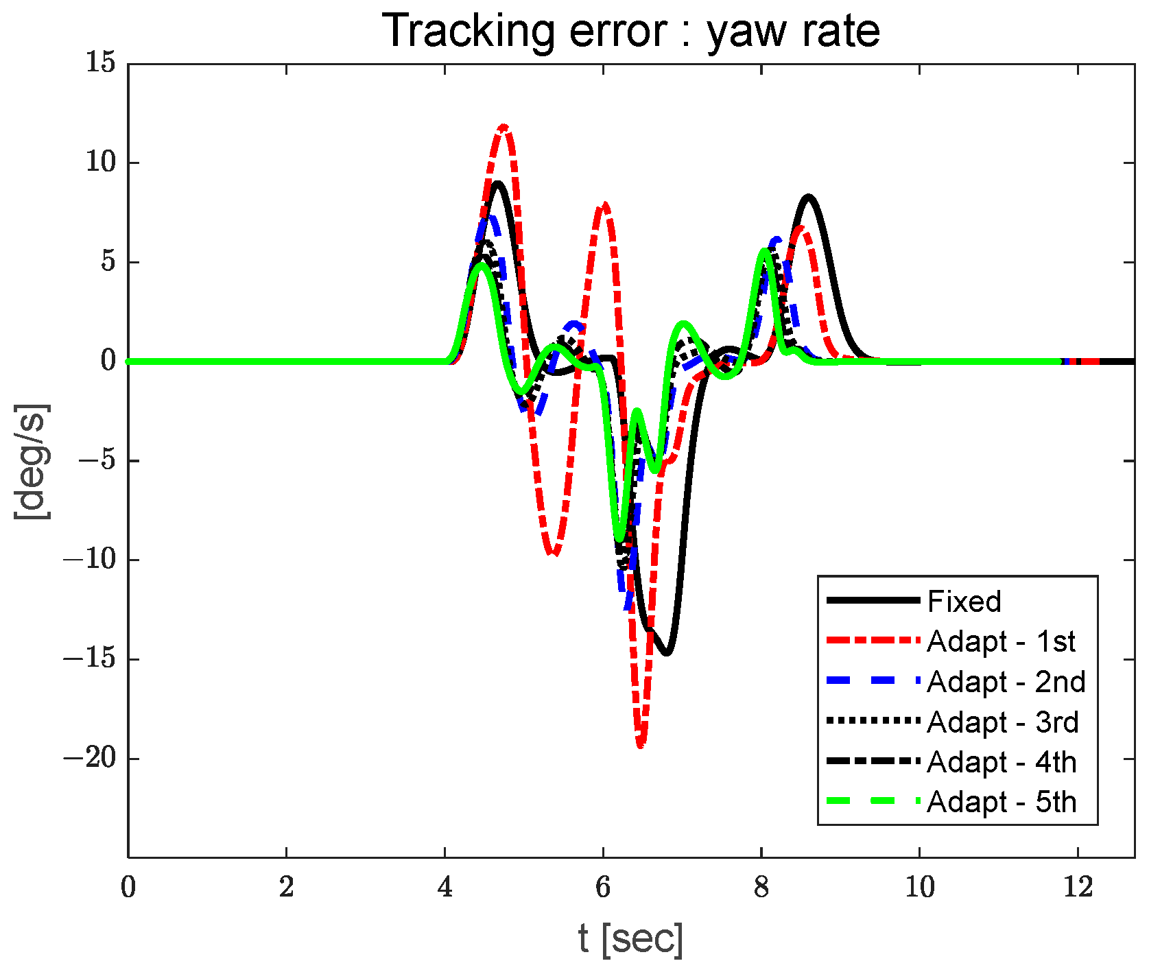
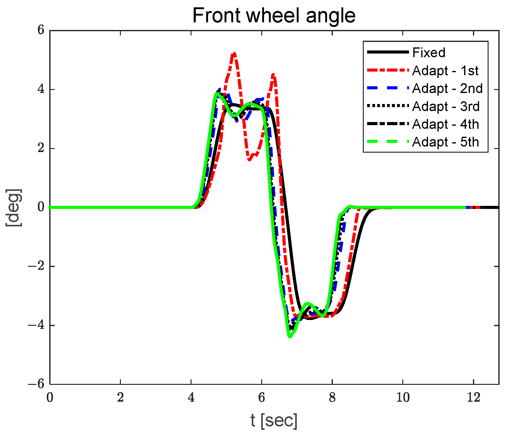
As shown in Figure 6, the yaw rate tracking error is decreased as the number of iterations for which evaluation increases. There is a relatively small overshoot phenomenon in the transient region of the target yaw rate, and the tracking error converges to zero after that region. Figure 7, Figure 8 and Figure 9 show the yaw rate tracking error, front wheel angle, and estimated coefficient.
It is observed that the oscillation phenomenon of the yaw rate tracking error and front wheel angle in Figure 7 and Figure 8 decreased as number of iterations for evaluation increased. In the case of the estimated coefficient b for yaw rate tracking, its value decreased as number of iterations for evaluation increased, and the oscillation phenomenon of the estimated value also decreased as number of iterations for evaluation increased. In case of the estimated coefficient a for yaw rate tracking, it was shown that there was a relatively large oscillation phenomenon in the transient region within 4~9 s. Figure 10 show the self-tuned proportional and integral gains.
The oscillation phenomenon of the yaw rate tracking error and front wheel angle can be observed in Figure 7 and Figure 8 to be decreased as the number of iterations for evaluation increases. In the case of the estimated coefficient b for yaw rate tracking, its value decreases as the number of iterations for evaluation increases, and the oscillation phenomenon of the estimated value also decreases as the number of iterations for evaluation increases. In the case of the estimated coefficient a for yaw rate tracking, it is shown that there is a relatively large oscillation phenomenon in the transient region within 4~9 s. Figure 10 shows the self-tuned proportional and integral gains.
The proportional gain is shown, revealing that there is a relatively large oscillation phenomenon in the transient region within 4~9 s, and the final gain values of each iteration for evaluation are around 0.2. It is shown that the oscillation phenomenon of the integral gain is decreased and gain value is the increased as number of iterations for evaluation is increased.
The proportional gain shows a relatively large oscillation phenomenon in the transient region within 4~9 s, and the final gain values of each iteration for evaluation are around 0.2.
As the iterative evaluations continued, the yaw rate tracking error and steering input oscillations steadily decreased (Figure 6, Figure 7 and Figure 8). Figure 6 shows a relatively small overshoot in the transient region, followed by a steady convergence to zero. Furthermore, Figure 7 and Figure 8 consistently show a gradual decrease in the tracking error and oscillations in the front wheel steering angle as the iterations progressed.
The changes in the estimated coefficients also showed consistent results. The estimated coefficient b decreased (shifted in the negative direction) with each iteration, reducing oscillations. Meanwhile, coefficient a showed relatively large fluctuations in the transient region (Figure 9). These coefficients and gain changes are well explained by the proposed self-tuning law (Equations (19)–(22)) and the trends in the estimated coefficients.
According to the derivation, k P is driven by the estimation coefficient a and the error integral e d t . In contrast, the other gains k I are driven by the estimation coefficient b and the immediate error e , respectively (Equations (21) and (22)). Due to iterative evaluation, the initial gain k P decreases after the transient period, naturally converging to a lower value. The other gains k I tend to increase proportionally with the decreasing estimation coefficients with each iteration (non-negativity constraints are applied in Equations (23) and (24)). Furthermore, the multi-forgetting RLS and rate limiter settings employed in this study effectively suppressed abrupt changes and fluctuations in gains and coefficients, thereby mitigating high-frequency gain oscillations and enhancing convergence across iterations despite the fluctuations observed during the transient period (Table 2).
In this experimental design, an iterative initialization approach was utilized in which the final PI gain obtained at the end of each iteration was used as the starting value for the following iteration. This strategy helped to accelerate the convergence process and effectively reduce oscillations in both the control signal and tracking error (Figure 4b). As a result, (i) a mitigation of error and steering input oscillation (Figure 6, Figure 7 and Figure 8), (ii) a stabilization of the estimation coefficients b and limited fluctuations a within the transient region (Figure 9), and (iii) a decrease k P and increase in the k I gain value (Figure 10) were causally linked, which enabled a fast convergence and low steady-state error after the transient region.

3.2. Longitudinal Velocity Tracking Results

Figure 11, Figure 12, Figure 13, Figure 14, Figure 15 and Figure 16 show the performance evaluation results for longitudinal velocity tracking.
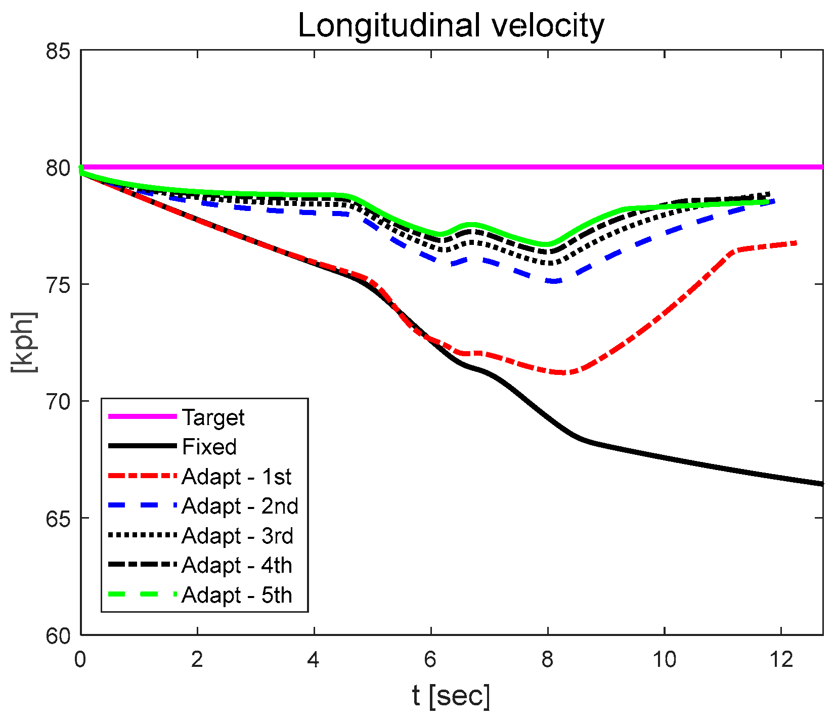
Figure 11 shows the longitudinal velocity of mobility according to the number of iterations for evaluation. It can be observed that the oscillation phenomenon of longitudinal velocity is decreased as the number of iterations for evaluation is increased. It can also be observed that the oscillation in longitudinal velocity decreases with an increasing number of evaluation iterations.
It is confirmed in Figure 12 that the longitudinal velocity tracking error is decreased as number of iterations for evaluation is increased. In the transient region within 2~9 s, there is a relatively large oscillation phenomenon, and tracking error convergence is decreased except for the transient region. Figure 13, Figure 14 and Figure 15 show the longitudinal velocity tracking error, front wheel torque, and estimated coefficient. There is a relatively large oscillation phenomenon in the transient region within 2~9 s, and the tracking error converges except for the transient region. Figure 13, Figure 14 and Figure 15 show the longitudinal velocity tracking error, front wheel torque, and estimated coefficient.
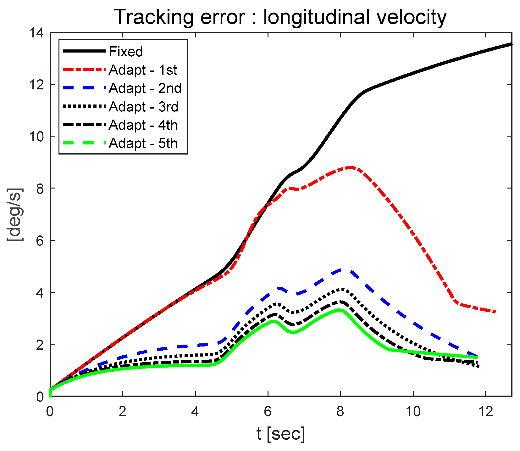
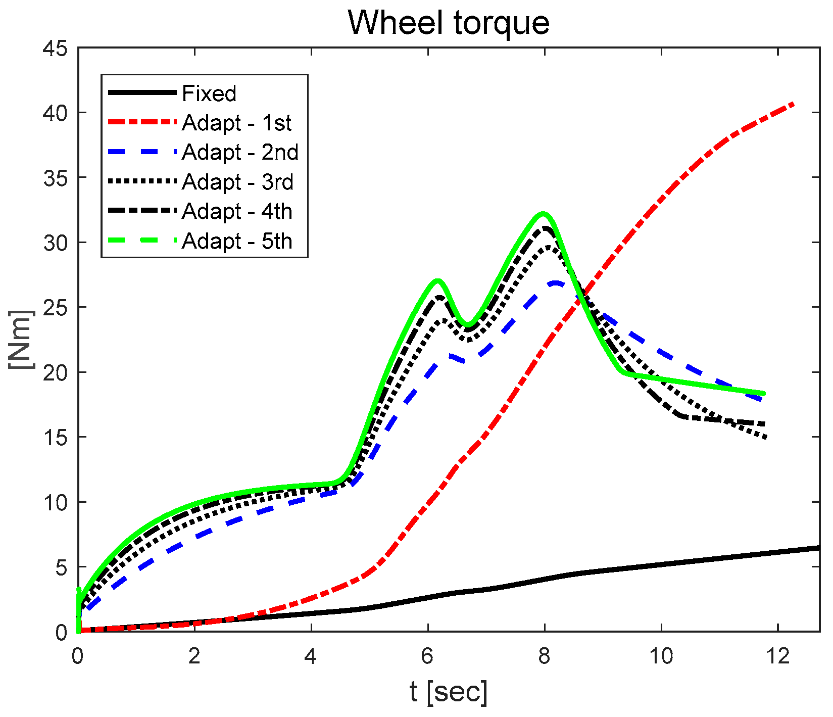
It can be observed in Figure 13 and Figure 14 that the tracking error of the longitudinal velocity is decreased and wheel torque is increased as number of iterations for evaluation is increased. In the case of the estimated coefficient a for longitudinal velocity tracking, its value is decreased as number of iterations for evaluation is increased, and there is a relatively small oscillation phenomenon of the estimated value for each iteration for evaluation. In the case of the estimated coefficient b for longitudinal velocity tracking, it is shown that there is no large difference between each iteration for evaluation, and final values are near −1.2. Figure 16 show the self-tuned proportional and integral gains.
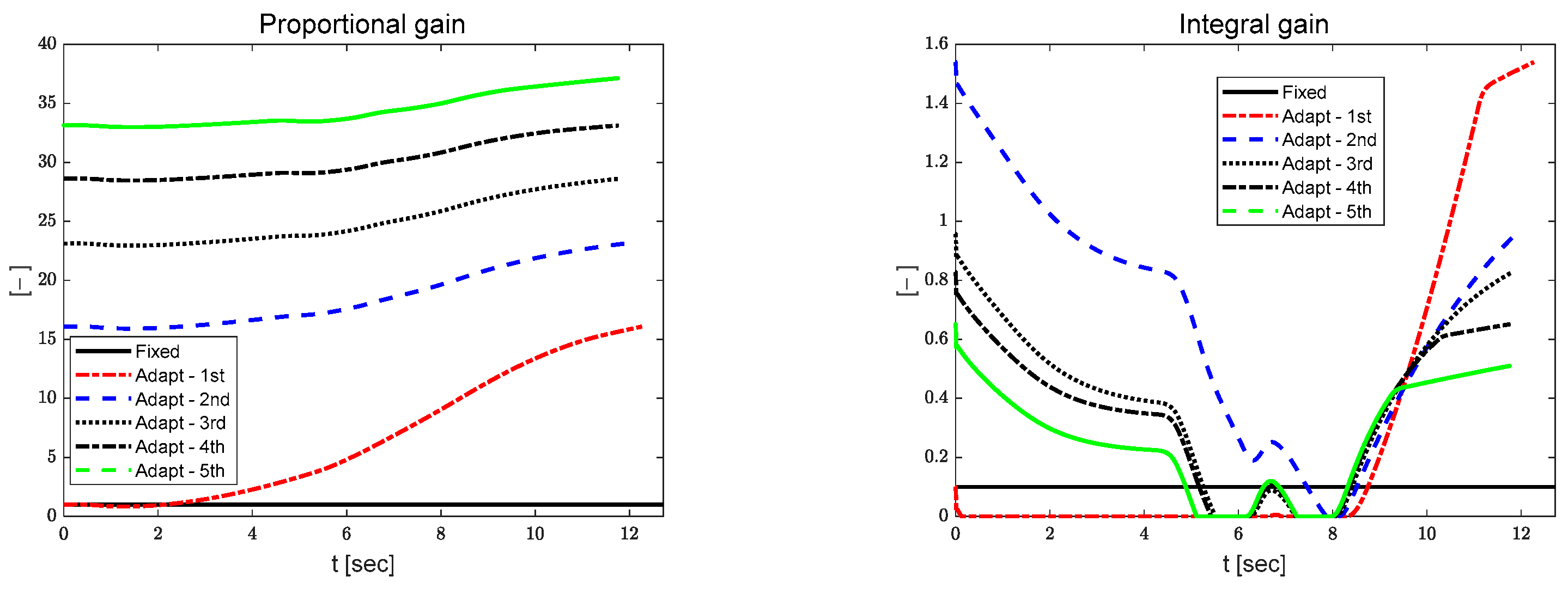
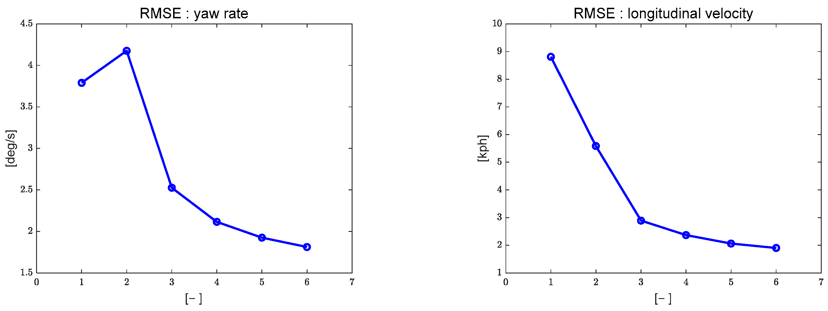
It is shown that the proportional gain is increased with the number of evaluation iterations, while the integral gain exhibits relatively large variations. Figure 17 presents the tracking error’s root mean square error (RMSE) for each evaluation iteration.
The horizon axis in Figure 17 represents the iteration for evaluation, and the vertical axis represents the yaw rate and longitudinal velocity tracking errors.
As the iterative evaluations progressed, longitudinal velocity oscillations were alleviated and tracking errors decreased (Figure 11, Figure 12 and Figure 13). Relatively large oscillations were observed, particularly in the transient period (2–9 s), but a clear trend of gradual convergence of errors was observed outside of this section. Furthermore, front-wheel drive torque exhibited an increasing trend with each iteration (Figure 14), which is consistent with the strengthening of the effective proportional action to suppress residual velocity errors after the transient. The changes in the estimated coefficients are causally linked to this phenomenon. In longitudinal velocity tracking, the coefficient a decreased with each iteration (resulting in relatively small oscillations). In contrast, coefficient b showed relatively small variation between iterations, converging to a final value of approximately −1.2 (Figure 15). The self-tuning gain (Figure 16) reflects this coefficient behavior, with k P increasing with each iteration and k I exhibiting relatively large variability. This is consistent with the structural consequence that a decreases with an increases k P , as seen in the gain-derived Equations (21) and (22).
In terms of quantitative metrics, the RMSE (Figure 17) confirms that the proposed self-tuning PID systematically improves the velocity-tracking performance. This evaluation concept uses the final PI gain from each iteration as the initial value for the next iteration (Figure 4b). The multi-forgetting RLS and rate limit settings (Table 3) suppress abrupt gain changes during the transient period, supporting the observed gradual increase in k P and the management of k I variability from a parameter design perspective.
In summary, we found the following: (i) error convergence after the transient period (2–9 s) (Figure 11, Figure 12 and Figure 13), (ii) that a decreased and b converged around −1.2 (Figure 15), (iii) that k P increased and there was k I variability (Figure 16), and (iv) iteration-based RMSE reduction (Figure 17). These form a consistent mechanism chain, showing that longitudinal velocity tracking is achieved faster and more stably as the iterative evaluation is repeated.

3.3. Yaw Rate Tracking Results with Disturbance and Noise

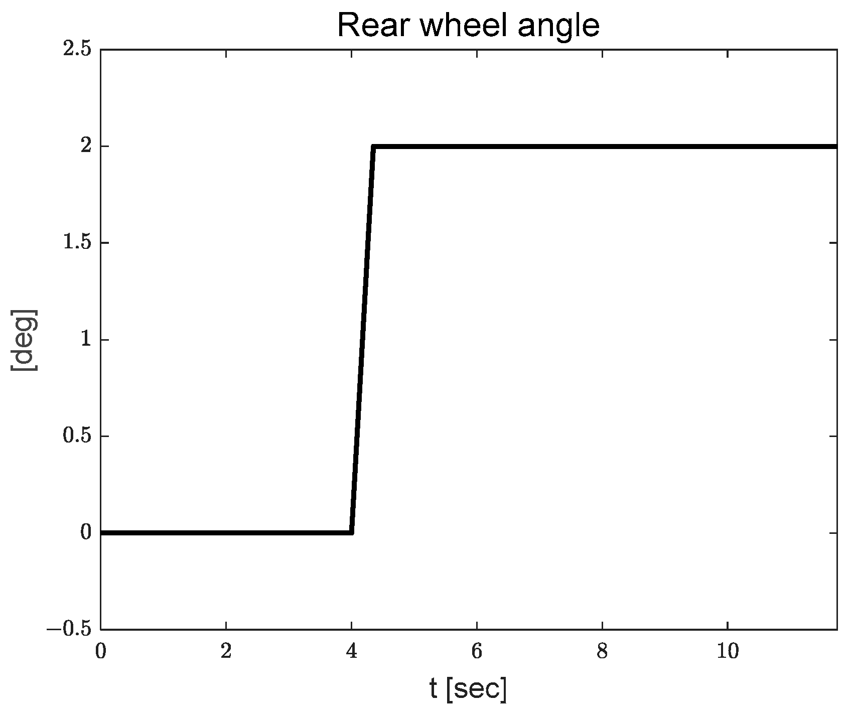
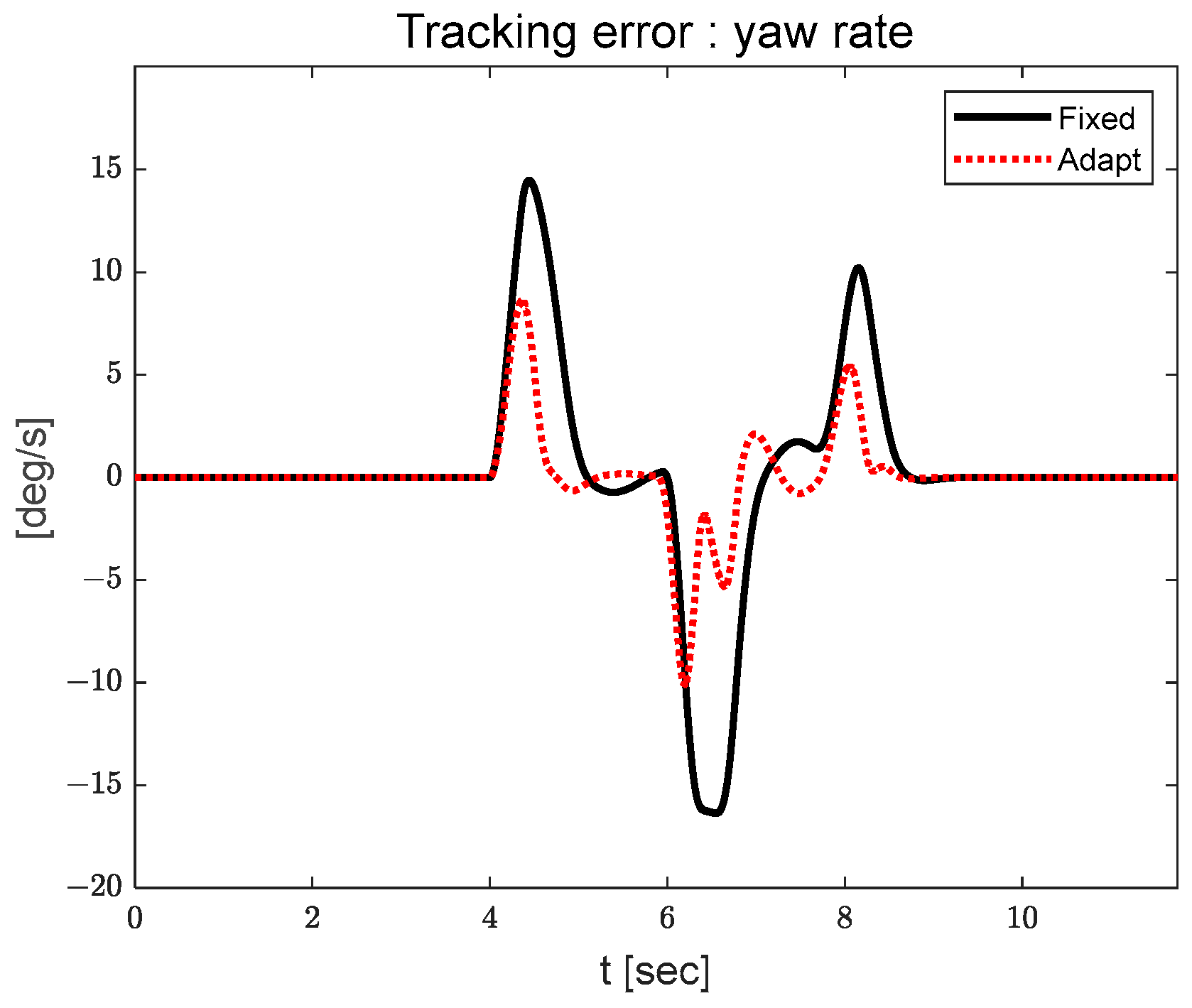
Performance evaluation of yaw rate tracking with disturbance was conducted, where the PID gains used for the fifth evaluation in the case of yaw rate tracking were used. The disturbance was designed so that the rear wheel angle was changed abruptly during evaluation. The disturbance applied to the evaluation is shown in Figure 18.
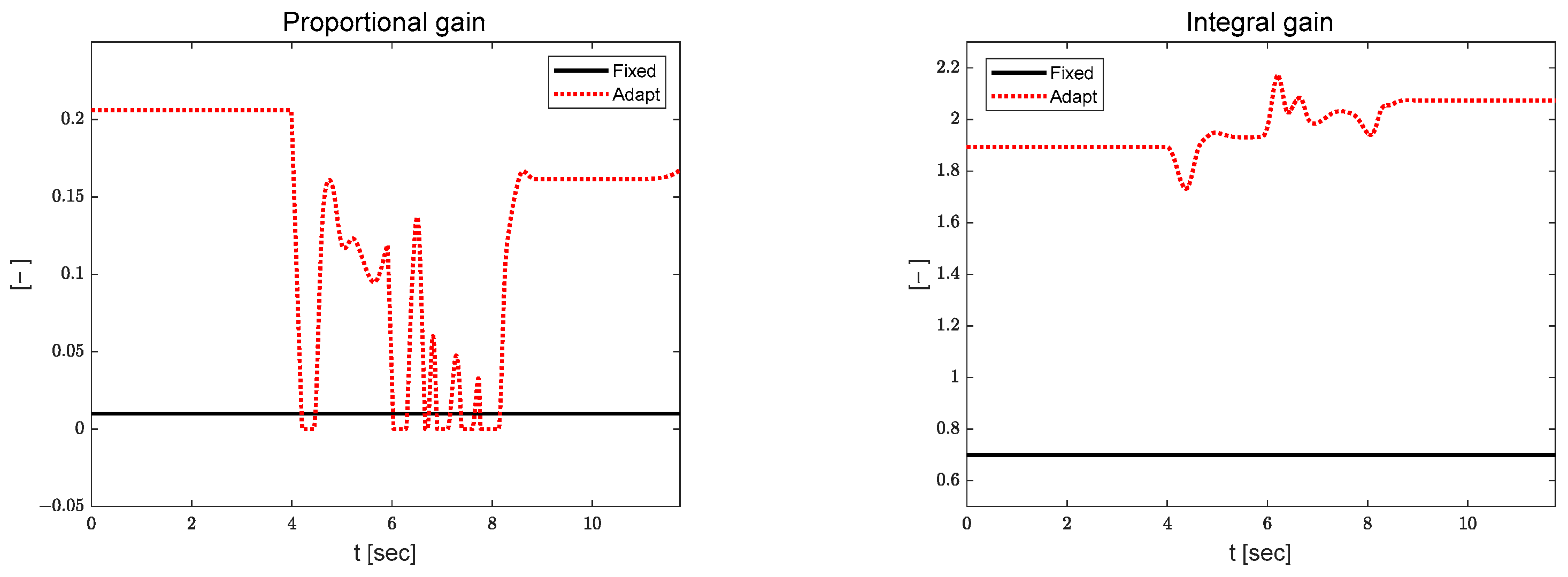
Figure 19 and Figure 20 show the performance evaluation results for yaw rate tracking with disturbance, depicting the tracking error and adapted PI gains, respectively.
As can be seen in Figure 19, the yaw rate tracking error in the case that is adapted is relatively smaller than in the case that is fixed despite the rear wheel angle disturbance. In Figure 20, it is shown that the proportional and integral gains are changed from 4 s with disturbance injection.

4. Conclusions

This study has presented an adaptive PID control algorithm that does not use a mathematical model for the yaw rate and longitudinal velocity tracking of various mobilities. To design the adaptive PID control algorithm, an error dynamic model was designed with coefficients to design the adaptive PID control algorithm, where the coefficients were estimated in real time by RLS with multiple forgetting factors. The Lyapunov direct method was used to derive proportional and integral gains with external conditions for the RLS. For a reasonable performance evaluation of the proposed adaptive PID control algorithm, the CarMaker software was used, and a path-tracking scenario was applied. The target yaw rate and longitudinal velocity were defined for path tracking, and two adaptive PID controllers were constructed for performance evaluation.
The S-curved path for tracking was used for evaluation, and iterative evaluation was conducted using the final gain from each evaluation as the initial gain for the subsequent evaluation. The evaluation results showed a reasonable tracking performance when using the proposed adaptive PID control algorithm. However, if there is signal noise and a delay, the control performance can be degraded, and the stability cannot be ensured. Therefore, the development of a derivative gain self-tuning algorithm with consideration of signal noise and delay effects is considered as a requirement for future work. Furthermore, because there are some limitations in the determination of the proper end point of gain self-tuning during iterations for evaluation and limited evaluation scenarios, evaluation under various scenarios and self-tuning decision algorithms based on optimization theories are also considered as future works of study. The proposed adaptive PID control framework, with appropriate modifications to the system model (Equation (1)) and regressor design (Equation (4)), can potentially be extended to a broader class of underactuated mechanical systems where Lyapunov-based gain mapping is applicable. However, the practical applicability depends on several conditions: (i) the error dynamics can be reasonably approximated by Equation (1), (ii) the PE condition is satisfied by the reference trajectory, and (iii) disturbances remain bounded within the ISS framework of Theorem 1. Further validation across diverse system types is necessary to establish general applicability.

Author Contributions

Conceptualization, J.L. and K.O.; Data Curation, J.L. and K.O.; Formal Analysis, J.L. and K.O.; Investigation, K.O.; Methodology, J.L. and K.O.; Resources, J.L. and K.O.; Software, J.L. and K.O.; Supervision, K.O.; Validation, J.L. and K.O.; Visualization, J.L. and K.O.; Writing—Original Draft, J.L. and K.O.; Writing—Review and Editing, J.L. and K.O. All authors have read and agreed to the published version of the manuscript.

Funding

This research received no external funding.

Data Availability Statement

The original contributions presented in this study are included in the article. Further inquiries can be directed to the authors.

Acknowledgments

The authors would like to thank the anonymous reviewers for their valuable comments and suggestions.

Conflicts of Interest

The authors declare no conflicts of interest.

Abbreviations

The following abbreviations are used in this manuscript:
PIDProportional Integral Derivative
RLSRecursive Least Squares
RLRate Limit

References

  1. Abdel-Aty, M.; Ding, S. A matched case-control analysis of autonomous vs. human-driven vehicle accidents. Nat. Commun. 2024, 15, 4931. [Google Scholar] [CrossRef]
  2. Jo, K.; Kim, J.; Kim, D.; Jang, C.; Sunwoo, M. Development of autonomous car—Part II: A case study on the implementation of an autonomous driving system based on distributed architecture. IEEE Trans. Ind. Electron. 2015, 62, 5119–5132. [Google Scholar] [CrossRef]
  3. Behere, S.; Törngren, M. A functional reference architecture for autonomous driving. Inf. Softw. Technol. 2016, 73, 136–150. [Google Scholar] [CrossRef]
  4. Coulter, R.C. Implementation of the Pure Pursuit Path Tracking Algorithm (No. CMURITR9201); The Robotics Institute Camegie Mellon University: Pittsburgh, PA, USA, 1992. [Google Scholar]
  5. Thrun, S.; Montemerlo, M.; Dahlkamp, H.; Stavens, D.; Aron, A.; Diebel, J.; Mahoney, P. Stanley: The robot that won the DARPA Grand Challenge. J. Field Robot. 2006, 23, 661–692. [Google Scholar] [CrossRef]
  6. Funke, J.; Brown, M.; Erlien, S.M.; Gerdes, J.C. Collision avoidance and stabilization for autonomous vehicles in emergency scenarios. IEEE Trans. Control. Syst. Technol. 2016, 25, 1204–1216. [Google Scholar] [CrossRef]
  7. He, Z.; Nie, L.; Yin, Z.; Huang, S. A two-layer controller for lateral path tracking control of autonomous vehicles. Sensors 2020, 20, 3689. [Google Scholar] [CrossRef]
  8. Menhour, L.; d’Andréa-Novel, B.; Fliess, M.; Gruyer, D.; Mounier, H. An efficient model-free setting for longitudinal and lateral vehicle control: Validation through the interconnected Pro-SiVIC/RTMaps prototyping platform. IEEE Trans. Intell. Transp. Syst. 2017, 19, 461–475. [Google Scholar] [CrossRef]
  9. Lee, K.; Jeon, S.; Kim, H.; Kum, D. Optimal path tracking control of autonomous vehicle: Adaptive full-state linear quadratic Gaussian (LQG) control. IEEE Access 2019, 7, 109120–109133. [Google Scholar] [CrossRef]
  10. Ahn, J.; Shin, S.; Kim, M.; Park, J. Accurate path tracking by adjusting look-ahead point in pure pursuit method. Int. J. Automot. Technol. 2021, 22, 119–129. [Google Scholar] [CrossRef]
  11. Gong, C.; Lu, C.; Li, Z.; Liu, Z.; Gong, J.; Chen, X. Beyond imitation: A life-long policy learning framework for path tracking control of autonomous driving. IEEE Trans. Veh. Technol. 2024, 73, 9786–9799. [Google Scholar] [CrossRef]
  12. Marino, R.; Scalzi, S.; Netto, M. Nested PID steering control for lane keeping in autonomous vehicles. Control. Eng. Pract. 2011, 19, 1459–1467. [Google Scholar] [CrossRef]
  13. Ma, Y.; Chen, J.; Wang, J.; Xu, Y.; Wang, Y. Path-tracking considering yaw stability with passivity-based control for autonomous vehicles. IEEE Trans. Intell. Transp. Syst. 2021, 23, 8736–8746. [Google Scholar] [CrossRef]
  14. Liang, Y.; Li, Y.; Zheng, L.; Yu, Y.; Ren, Y. Yaw rate tracking-based path-following control for four-wheel independent driving and four-wheel independent steering autonomous vehicles considering the coordination with dynamics stability. Proc. Inst. Mech. Eng. Part D J. Automob. Eng. 2020, 235, 260–272. [Google Scholar] [CrossRef]
  15. Wang, X.; Fu, M.; Ma, H.; Yang, Y. Lateral control of autonomous vehicles based on fuzzy logic. Control. Eng. Pract. 2015, 34, 1–17. [Google Scholar] [CrossRef]
  16. Paden, B.; Čáp, M.; Yong, S.Z.; Yershov, D.; Frazzoli, E. A survey of motion planning and control techniques for self-driving urban vehicles. IEEE Trans. Intell. Veh. 2016, 1, 33–55. [Google Scholar] [CrossRef]
  17. Yao, Q.; Tian, Y. A model predictive controller with longitudinal speed compensation for autonomous vehicle path tracking. Appl. Sci. 2019, 9, 4739. [Google Scholar] [CrossRef]
  18. Lin, F.; Chen, Y.; Zhao, Y.; Wang, S. Path tracking of autonomous vehicle based on adaptive model predictive control. Int. J. Adv. Robot. Syst. 2019, 16, 1729881419880089. [Google Scholar] [CrossRef]
  19. Zhu, K.; Yu, C.; Wan, Y. Recursive Least Squares Identification with Variable-Direction Forgetting via Oblique Projection Decomposition. IEEE/CAA J. Autom. Sin. 2021, 9, 547–555. [Google Scholar] [CrossRef]
  20. Sarhadi, P.; Noei, A.R.; Khosravi, A. Model reference adaptive PID control with anti-windup compensator for an autonomous underwater vehicle. Robot. Auton. Syst. 2016, 83, 87–93. [Google Scholar] [CrossRef]
  21. Garpinger, O.; Haggl, T. Software-based optimal PID design with robustness and noise sensitivity constraints. J. Process Control. 2015, 33, 90–101. [Google Scholar] [CrossRef]
  22. Chu, D.; Li, H.; Zhao, C.; Zhou, T. Trajectory tracking of autonomous vehicle based on model predictive control with PID feedback. IEEE Trans. Intell. Transp. Syst. 2022, 24, 2239–2250. [Google Scholar] [CrossRef]
  23. Liu, Q.; Gordon, T.; Rahman, S. Model-free autonomous control of four-wheel steering using artificial flow guidance. Veh. Syst. Dyn. 2023, 62, 1565–1586. [Google Scholar] [CrossRef]
  24. Tork, N.; Amirkhani, A.; Shokouhi, S.B. An adaptive modified neural lateral-longitudinal control system for path following of autonomous vehicles. Eng. Sci. Technol. Int. J. 2021, 24, 126–137. [Google Scholar] [CrossRef]
  25. Shan, Y.; Zheng, B.; Chen, L.; Chen, L.; Chen, D. A reinforcement learning-based adaptive path tracking approach for autonomous driving. IEEE Trans. Veh. Technol. 2020, 69, 10581–10595. [Google Scholar] [CrossRef]
  26. Tang, M.; Chen, X.; Tang, K.; Zhang, Y.; Wang, W. Longitudinal and Lateral Cooperative Control of Preview Intelligent Vehicles with Stabilization. J. Intell. Robot. Syst. 2024, 110, 156. [Google Scholar] [CrossRef]
  27. Zeng, D.; Pan, S.; Yu, Y.; Hu, Y.; Yang, J.; Zhang, P.; Gao, L. A comparative study on trajectory tracking control methods for automated vehicles. Sci. Rep. 2025, 15, 17073. [Google Scholar] [CrossRef]
  28. Simorgh, A.; Marashian, A.; Razminia, A. Adaptive pid control design for longitudinal velocity control of autonomous vehicles. In Proceedings of the 2019 6th International Conference on Control, Instrumentation and Automation (ICCIA), Sanandaj, Iran, 30–31 October 2019; pp. 1–16. [Google Scholar]
  29. Sun, D.; Hu, S.; Shao, X.; Liu, C. Global stability of a saturated nonlinear PID controller for robot manipulators. IEEE Trans. Control. Syst. Technol. 2009, 17, 892–899. [Google Scholar] [CrossRef]
  30. Jafarov, E.M.; Parlakçi, M.N.A.; Istefanopulos, Y. A new variable structure PID-controller design for robot manipulators. IEEE Trans. Control. Syst. Technol. 2005, 13, 122–130. [Google Scholar] [CrossRef]
  31. Yamamoto, T.; Takao, K.; Yamada, T. Design of a data-driven PID controller. IEEE Trans. Control. Syst. Technol. 2008, 17, 29–39. [Google Scholar] [CrossRef]
  32. Li, X.H.; Yu, H.B.; Yuan, M.Z. Design of an optimal PID controller based on Lyapunov approach. In Proceedings of the 2009 International Conference on Information Engineering and Computer Science, Los Angeles, CA, USA, 31 March–2 April 2009; pp. 1–5. [Google Scholar]
  33. Norlund, F.; Hagglund, T.; Soltesz, K. Seamless PID–MPC hybrid control. In Proceedings of the 4th IFAC Conference on Advances in Proportional-Integral-Derivate Control PID 2024, Almería, Spain, 12–14 June 2024; Volume 58, pp. 19–24. [Google Scholar]
  34. Saat, S.; Ahmad Mohd Ghazali, M. Data-driven brain emotional learning-based intelligent controller-PIDcontrol of MIMO systems based on a modified safe experimentation dynamics algorithm. Int. J. Cogn. Comput. Eng. 2025, 6, 74–99. [Google Scholar]
  35. Vahidi, A.; Stefanopoulou, A.; Peng, H. Recursive least squares with forgetting for online estimation of vehicle mass and road grade: Theory and experiments. Veh. Syst. Dyn. 2005, 43, 31–55. [Google Scholar] [CrossRef]
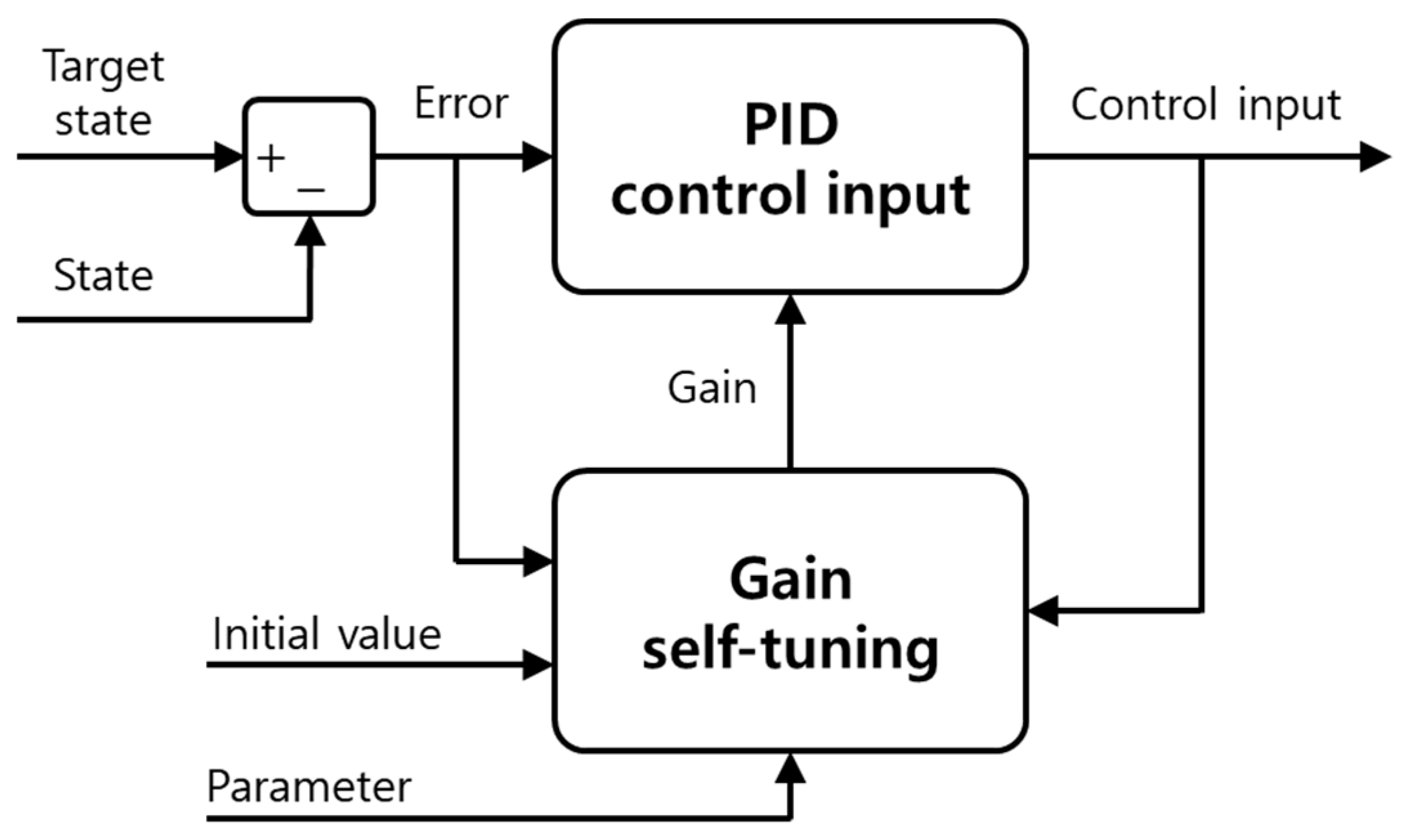
Figure 1. Block diagram of the proposed adaptive PID control algorithm.
Electronics 14 04111 g001
Figure 2. Detailed block diagram of the gain self-tuning algorithm with constraints.
Electronics 14 04111 g002
Figure 3. Target path (left) and target values (right): longitudinal velocity and yaw rate.
Electronics 14 04111 g003
Figure 4. Block diagram and evaluation concept for performance evaluation using CarMaker. (a) Overall diagram for evaluation. (b) Overall diagram for evaluation.
Electronics 14 04111 g004
Figure 5. Result: yaw rate.
Electronics 14 04111 g005
Figure 6. Results: target and current yaw rate ((a)—1st, (b)—2nd, (c)—3rd, (d)—4th, (e)—5th). (a) First driving. (b) Second driving. (c) Third driving. (d) Fourth driving. (e) Fifth driving.
Electronics 14 04111 g006aElectronics 14 04111 g006b
Figure 7. Result: yaw rate tracking error.
Electronics 14 04111 g007
Figure 8. Result: front wheel angle.
Electronics 14 04111 g008
Figure 9. Result: estimated coefficient for yaw rate tracking (left—a, right—b).
Electronics 14 04111 g009
Figure 10. Result: gain for yaw rate tracking (left—proportional, right—integral).
Electronics 14 04111 g010
Figure 11. Result: longitudinal velocity (target velocity—80 kph).
Electronics 14 04111 g011
Figure 12. Results: target and current velocity ((a)—1st, (b)—2nd, (c)—3rd, (d)—4th, (e)—5th). (a) First driving. (b) Second driving. (c) Third driving. (d) Fourth driving. (e) Fifth driving.
Electronics 14 04111 g012aElectronics 14 04111 g012b
Figure 13. Result: longitudinal velocity tracking error.
Electronics 14 04111 g013
Figure 14. Result: wheel torque.
Electronics 14 04111 g014
Figure 15. Result: estimated coefficient for longitudinal velocity tracking (left—a, right—b).
Electronics 14 04111 g015
Figure 16. Result: gain for longitudinal velocity tracking (left—proportional, right—integral).
Electronics 14 04111 g016
Figure 17. Result: RMSE for each evaluation (left—yaw rate error, right—longitudinal velocity).
Electronics 14 04111 g017
Figure 18. Disturbance: rear wheel angle (start changing from 4 s).
Electronics 14 04111 g018
Figure 19. Result: yaw rate tracking error (with disturbance).
Electronics 14 04111 g019
Figure 20. Result: gain (left—proportional, right—integral).
Electronics 14 04111 g020
Table 1. Main vehicle parameters.
ParameterValueUnit
Mass2275Kg
Wheel base2.975m
Distance between mass center and front axle1.324m
Distance between mass center and rear axle1.651m
Road surfaceDry asphalt-
Tire cornering stiffness (front/rear)75,000/140,000N/rad
Table 2. Main adaptive PID control parameters used for yaw rate tracking evaluation.
ParameterValueRemark
Initial estimate−0.025/−0.7Proportional/Integral
Initial covariance0.01-
Forgetting factor0.995/0.9995Proportional/Integral
Rate limit1/2Proportional/Integral
Weighting factor0.01-
Reduction rate0.01-
Fixed proportional gain0.01-
Fixed integral gain0.7-
Derivative gain0.0001-
Table 3. Main adaptive PID control parameters used for longitudinal velocity tracking evaluation.
ParameterValueRemark
Initial estimate−0.025/−0.7Proportional/Integral
Initial covariance0.01-
Forgetting factor0.995/0.9995Proportional/Integral
Rate limit1/2Proportional/Integral
Weighting factor0.01-
Reduction rate0.01-
Fixed proportional gain1-
Fixed integral gain0.1-
Derivative gain0.01-
Disclaimer/Publisher’s Note: The statements, opinions and data contained in all publications are solely those of the individual author(s) and contributor(s) and not of MDPI and/or the editor(s). MDPI and/or the editor(s) disclaim responsibility for any injury to people or property resulting from any ideas, methods, instructions or products referred to in the content.