Article

TTBCA+: An Enhanced Besiege and Conquer Algorithm with Three-Three Tactics and Collision Theory for Complex Optimization Problems

School of Management Science and Information Engineering, Jilin University of Finance and Economics, Changchun 130117, China
*
Author to whom correspondence should be addressed.
Electronics 2025, 14(20), 4051; https://doi.org/10.3390/electronics14204051
Submission received: 15 September 2025 / Revised: 6 October 2025 / Accepted: 13 October 2025 / Published: 15 October 2025
(This article belongs to the Special Issue AI Applications of Multi-Agent Systems)

Abstract

Besiege and Conquer Algorithm (BCA) is a swarm intelligence algorithm proposed in 2025 based on tactical concepts. However, its besiege and conquer strategies have some problems, such as insufficient diversity and local stagnation. To solve the above problems, this paper proposes an Enhanced Besiege and Conquer Algorithm with Three-Three Tactics and Collision Theory, referred to as TTBCA+. TTBCA+ has four innovations. Firstly, a three-three allocation mechanism of battlefield and roles is proposed to enhance its besiege capability; secondly, a three-three deployment mechanism of soldiers is proposed to enhance its conquer capability; thirdly, the balance factor between exploration and exploitation is modified for three-three tactics implementation; finally, the collision mechanism from collision theory is introduced to deal with soldiers beyond the search space. The performance of the proposed TTBCA+ is verified at the IEEE CEC 2017 and IEEE CEC 2022 benchmark functions, compared with 13 swarm intelligence algorithms, including classical algorithms, well-known algorithms such as JADE, lshade_rsp, AGWO, and recent 5 years algorithms, such as BCA, HOA, PLO, CFOA, HLOA, DBO, BOA. Meanwhile, the proposed algorithms are applied to two practical complex optimization problems. The results show that TTBCA+ effectively solved the limitations in BCA, and it is superior to other compared algorithms.

1. Introduction

In the process of solving complex optimization problems, swarm intelligence algorithms, as an important branch in the field of artificial intelligence, have gradually increased in importance [1]. Such algorithms are usually inspired by the behaviors of biological groups in nature, such as flocks of birds foraging [2], colonies of bees gathering nectar [3], tree seeds evolution [4], etc. In recent years, meta-heuristic algorithms have emerged in an endless stream, and an increasing number of scholars have improved the classical algorithms of swarm intelligence to enhance performance, such as MIAO [5], BWOA [6], MOBCA [7], fb-TSA [8],DTSA [9], and ADTSA [10]. These classic or improved algorithms often have inherent limitations due to the restricted cognitive capacity of search agency and cooperation mechanism [11]. However, war is cruel. Military tactical concepts are the crystallization of human wisdom, and the application of tactics often determines the direction and outcome of war. In the long term practice of war, human beings have accumulated a lot of war experience and summarized many tactical concepts full of wisdom. To this end, Jiang proposed the Besiege and Conquer Algorithm, named BCA in 2025 [12], which makes up for the deficiencies of swarm intelligence algorithms in the field of warfare by simulating military tactical concepts, and stood out among many algorithms. This algorithm is inspired by traditional warfare and simulates the combat behaviors of armies and soldiers on the battlefield, highlighting the tactical concept of concentrating superior forces to besiege the enemy, and the issue of balancing the front and the rear behind enemy lines was taken into consideration [12]. In addition, BCA also has the advantage of having fewer parameters, with only one balance factor—BCB. Meanwhile, the structure of BCA is very clear, which includes besiege strategy, conquer strategy, balance strategy, and feedback strategy. Finally, BCA is highly suitable for solving complex optimization problems, and it has been verified on multiple practical problems such as IEEE CEC benchmark functions and engineering examples, proving its significant superiority in exploration, exploitation, convergence capability, and application prospects [12].
However, BCA still mainly has the following problems. First, in the besiege strategy, the search mode of soldiers lacks diversity. All soldiers have the same generation mechanism with no role difference, resulting in insufficient population diversity. Hence, the coverage of the search space is not comprehensive. Second, in the conquer strategy, it is easy to fall into local optimum without a local-aware escape strategy. In BCA, the way to escape the local optimal solution depends on dynamic adjustment of balance factor BCB. However, the BCB factor is not an adaptive mechanism. Therefore, soldiers have less opportunity to approach the global optimal solution in a more complex search space. Third, large repetitive searches of a certain area result in a waste of resources. In high-dimensional complex problems, the generation methods of soldiers in BCA only rely on the dynamic adjustment of disturbance coefficients k1 and k2, so the search paths of soldiers lack direction, and the solution distribution in the search space is too dense. Fourth, the original regenerate way of the soldiers who, beyond the search space, disrupted the continuity of the search process.
Thus, this paper proposed an Enhanced Besiege and Conquer Algorithm with Three-Three Tactics and Collision Theory, named as TTBCA+. First, we proposed a three-three allocation mechanism of battlefield and roles to improve the diversity of search strategies. Second, we proposed a three-three position deployment mechanism of soldiers to increase the capability to escape the local optimum, increase the coverage capability of search space, and reduce repetitive searches. Third, we modified the balance factor BCB to balance exploration and exploitation. Fourth, we proposed a collision mechanism to improve the continuity of the search process. These above four innovations of BCA have made the algorithm more suitable for solving complex optimization problems.
The rest of this paper can be divided into the following sections: BCA and the three-three tactics are introduced in Section 2. The improvements of BCA are proposed in Section 3. The experimental results of TTBCA+ are presented and analyzed at IEEE CEC 2017 and IEEE CEC 2022 benchmark functions in Section 4. Applications of TTBCA+ in engineering design problems are shown in Section 5. Finally, the discussion of the algorithm and the conclusions are reported in Section 6.

2. Related Work

TTBCA+ enhances BCA with the inspiration from the three-three tactics. BCA is introduced in Section 2.1, and the three-three tactics is depicted in Section 2.2.

2.1. BCA: Besiege and Conquer Algorithm

BCA was proposed by Jiang from Jilin University of Finance and Economics in 2025 [12]. It is a swarm intelligence algorithm inspired by traditional warfare. In BCA, the army positions represent possible solutions to the optimization problem. BCA generates the positions of soldiers through two formulas, balances exploration and exploitation through balance factor BCB. This subsection will introduce the BCA algorithm in detail. At the beginning, Equation (1) is used to initialize the army in the search space.
A i , d = l b + ( u b l b ) × r a n d
where A i , d is the i t h army of the d t h dimension, l b and u b are the lower and upper bounds of the search space, and r a n d is a random constant in the range of [0, 1].
In BCA, the generated rules are Equations (2) and (3). Equation (2) mainly takes into account the current army position and the best army position, focusing on local search. Equation (3) uses two different army positions, namely the current army and the random army, to generate the soldier positions, focusing on global search. By comparing the relationship between the B C B and the r a n d , it is determined how to generate the positions of the soldiers. Specifically, if r a n d is less than BCB, Equation (2) is used to generate the position of soldiers. Otherwise, Equation (3) is used to generate the position of soldiers.
S j , d t + 1 = B d t + | A r , d t A i , d t | × k 1
S j , d t + 1 = A r , d t + | A r , d t A i , d t | × k 2
k 1 = sin ( 2 × π × r a n d )
k 2 = cos ( 2 × π × r a n d )
where S j , d t + 1 is the j t h soldier of the d t h dimension with ( t + 1 ) t h iteration, B d t is the current best army of the d t h dimension with t t h iteration, A r , d t is a random army of the d t h dimension with t t h iteration, A i , d t is the i t h army of the d t h dimension with t t h iteration, and both k 1 and k 2 are the disturbance coefficients. It should be noted that, in BCA, after initialization, each army has three soldiers.
The soldiers that are beyond the search space should be regenerated. Therefore, in BCA, if there are soldiers beyond the search space, in order to improve the population diversity and the exploration capability of soldiers when beyond the boundary, BCA generates the positions of the soldiers beyond the boundary through Equation (6) to (7).
Equation (6) focuses on the best army and the current army, and it can enhance the diversity of global search. If soldiers are generated by Equation (2) and some of them are beyond the search space, we use Equation (6) to regenerate these soldiers.
In addition, discarding soldiers beyond the search space range will reduce population diversity and slow down the convergence rate. Thus, if soldiers are generated by Equation (3) and some of them are beyond the search space, we use Equation (7) to regenerate soldiers randomly.
S j , d t + 1 = B C B t × B d t + ( 1 B C B t ) × A i , d t
S j , d t + 1 = l b + ( u b l b ) × r a n d
where B C B t is the value of B C B of t t h iteration.

2.2. The Three-Three Tactics

The three-three tactics is an advanced besiege and conquer tactics, which has the advantages of reducing the loss of soldiers in the attack and having a small number of soldiers form an encirclement situation.
The basic principle of the three-three tactics is to divide the army into three squads. Each squad is further divided into three fire teams. Each fire team consists of three soldiers: one assault soldier, one cover soldier, and one support soldier. This mode can ensure the concentration of superior forces while appropriately extending the front line, dispersing soldiers, and improving combat efficiency and survival ability.

3. Methods

Inspired by the three-three tactics, this section proposes three mechanisms to solve the problems of BCA. First, we introduce the three-three allocation mechanism of battlefield and roles, dividing the battlefield into the front and the area behind enemy lines and classifying soldiers into assault role, cover role, and support role to achieve clear division among soldiers. Second, we propose the three-three position deployment mechanism of soldiers, centering on the current optimal solution, forming a three-layer encirclement structure. The soldiers in each layer of the enclosure are deployed according to this mechanism to enhance the local search capability. Third, we propose a collision mechanism, bouncing the soldiers beyond the boundary back into the search space to maintain the continuity of the search process. Finally, by integrating these mechanisms, TTBCA+ is proposed.

3.1. Three-Three Allocation Mechanism of Battlefield and Roles

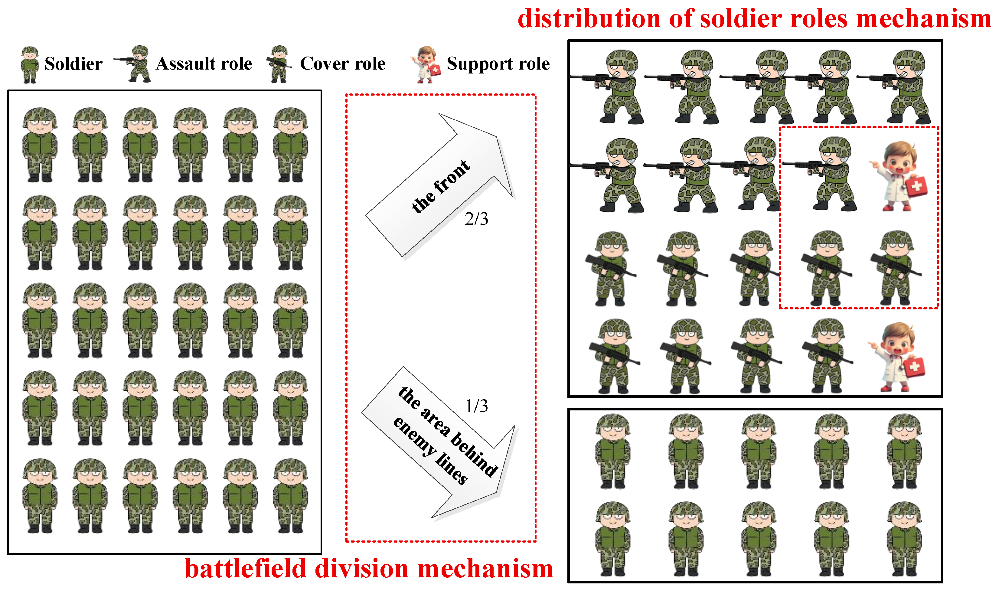
In order to improve the diversity of soldiers, the ideas of regional control as well as soldiers cooperate with each other in three-three tactics were introduced, which is the three-three allocation mechanism of battlefield and roles. It consists of the battlefield division mechanism and the distribution of soldier roles mechanism. Firstly, the battlefield is divided into the front and the area behind enemy lines. To implement the distribution principle of concentrating superior forces in three-three tactics, soldiers are allocated in a ratio of 2:1. Specifically, two-thirds of the soldiers are allocated to the front to besiege and conquer the enemy, and the other soldiers are allocated to the area behind enemy lines to interfere with the enemy. To achieve this distribution principle and balance the front and the rear behind enemy lines, BCB is set to an approximate value of two-thirds, that is, 0.6.
Secondly, we allocate the soldiers on the battlefield. Like three-three tactics, soldiers have three roles, including assault role, cover role, and support role. Assault role is responsible for besieging the enemy, the cover role is responsible for covering the assault role with firepower, and the support role is responsible for supporting the assault role and the cover role as well as causing disturbances on the area behind enemy lines. In order to ensure that the front has the strongest firepower to annihilate the enemy, all assault soldiers, cover soldiers, and a few of support soldiers are allocated to the front.
Through this clear division, different soldiers have different missions, which solves the deficiency of the besiege strategy lacks diversity in BCA. Soldiers can encircle and annihilate the enemy more purposefully, making local search more regular and efficient. This mechanism is shown in Figure 1.

3.2. Three-Three Position Deployment Mechanism of Soldiers

Three-three position deployment mechanism of soldiers is a mechanism for deploying the positions of assault role and cover role.
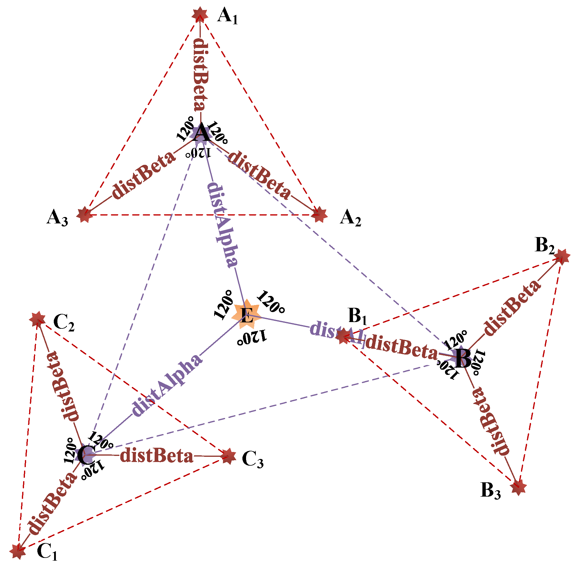
The first step, as shown in Figure 2, is to take the current optimal solution ( E n e m y , E ) as the center and generate a reference point A with a random angle and a random Euclidean Distance from the optimal solution through Equations (8) and (11). Then, we use Equations (9) and (11) to generate a reference point B, which forms a 120-degree with the reference point A and has a random Euclidean Distance from the optimal solution. Finally, we use Equations (10) and (11) to generate a reference point C, which forms a 240-degree with the reference point A and has a random Euclidean Distance from the optimal solution. We generate the first layer of reference points based on the above step to cover the potential optimal areas on a large scale.
a n g A l p h a d t = r a n d × 2 × π
a n g B e t a d t = a n g A l p h a d t + 2 3 × π
a n g D e l t a d t = a n g A l p h a d t + 2 × 2 3 × π
d i s t A l p h a d t = ( B d t A i , d t ) + r a n d 1 + α × t
where a n g A l p h a d t is the angle of the first reference point of each layer, such as A, A 1 , A 1 of d t h dimension with t t h iteration, a n g B e t a d t is the angle of the second reference point of each layer, such as B, B 1 , B 1 of d t h dimension with t t h iteration, a n g D e l t a d t is the angle of the third reference point of each layer such as C, C 1 , C 1 of d t h dimension with t t h iteration, and d i s t A l p h a d t is the Euclidean Distance between the first layer reference points, such as A, B, C, and the enemy of d t h dimension with t t h iteration, α = 0.1.
The second step, as shown in Figure 3, takes reference point A as the center and generates a reference point A 1 with a random angle and a random Euclidean Distance from the reference point A through Equations (8) and (12). Then, we use Equations (9) and (12) to generate a reference point A 2 , which forms a 120-degree with the reference point A 1 and has a random Euclidean Distance from the reference point A. Finally, we use Equations (10) and (12) to generate a reference point A 3 , which forms a 240-degree with the reference point A 1 and has a random Euclidean Distance from the A. Similarly, we take other reference points B and C as the center respectively and generate six second layer reference points B 1 , B 2 , B 3 , C 1 , C 2 , C 3 form the second layer of reference points to refine the search range.
d i s t B e t a d t = d i s t A l p h a d t × 1 3 + r a n d 1 + α × t
where d i s t B e t a d t is the Euclidean Distance between the second layer reference points, such as A 1 , B 1 , C 1 , and the enemy of d t h dimension with t t h iteration.
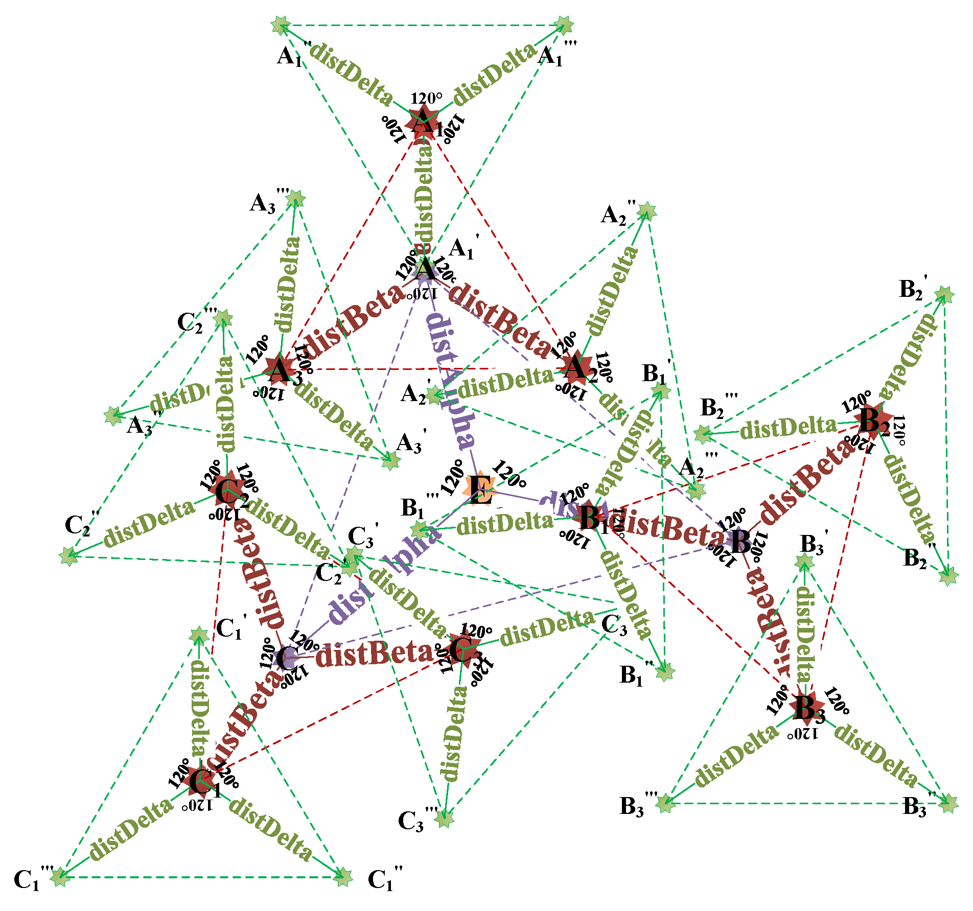
The third step, as shown in Figure 4, takes reference point A 1 as the center and generate a reference point A 1 with a random angle and a random Euclidean Distance from the reference point A 1 through Equations (8) and (13). Then, we use Equations (9) and (13) to generate a reference point A 1 , which forms a 120-degree with the reference point A 1 and has a random Euclidean Distance from the reference point A 1 . Finally, we use Equations (10) and (13) to generate a reference point A 1 , which forms a 240-degree with the reference point A 1 and has a random Euclidean Distance from the reference point A 1 . Similarly, we take other reference points A 2 , A 3 , B 1 , B 2 , B 3 , C 1 , C 2 , C 3 as the center, respectively, and generate twenty-four third-layer reference points A 2 , A 2 , A 2 , A 3 , A 3 , A 3 , B 1 , B 1 , B 1 , B 2 , B 2 , B 2 , B 3 , B 3 , B 3 , C 1 , C 1 , C 1 , C 2 , C 2 , C 2 , C 3 , C 3 , C 3 , forming the third layer of reference points to refine the search range.
d i s t D e l t a d t = d i s t B e t a d t × 1 3 + r a n d 1 + α × t
where d i s t D e l t a d t is the Euclidean Distance between the third layer reference points, such as A 1 , B 1 , C 1 , and the enemy of d t h dimension with t t h iteration.
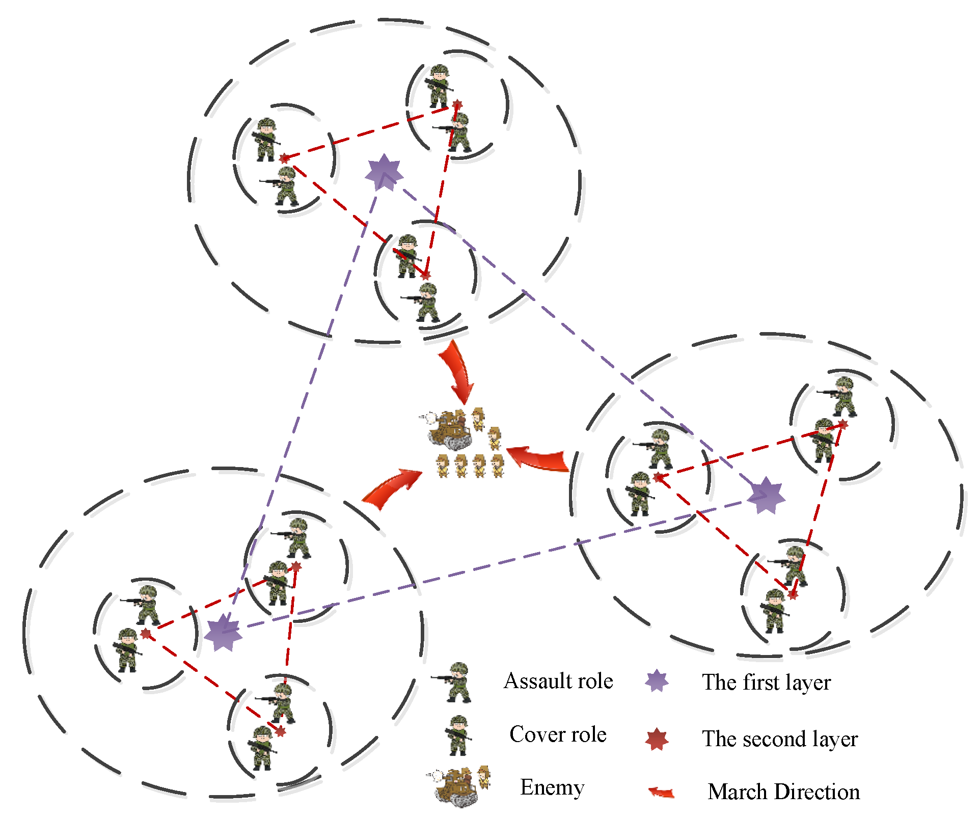
The last step, as shown in Figure 5, the positions of nine assault soldiers are selected through Equation (14), and the positions of nine cover soldiers are selected through Equation (15). Eventually, a three-layer encirclement structure is formed. This regular and flexible deployment method not only enhances the ability to cover the solution space, but also strengthens the ability to encircle and conquer the enemy through layer-by-layer advancement. Soldiers search for the optimal solution according to this deployment mode, which makes up for the shortcomings of wasted soldier resources and random distribution of soldier positions in BCA, enhances the local search capability of the algorithm, accelerates the convergence speed of the algorithm, and enables it to approach the global optimal solution more quickly.
A s l t P o s t d t = B d t + d i s t A l p h a d t × sin ( a n g A l p h a d t ) + d i s t B e t a d t × sin ( a n g B e t a d t ) + d i s t D e t a d t × sin ( a n g D e l t a d t )
C o v P o s t d t = B d t + d i s t A l p h a d t × sin ( a n g A l p h a d t ) + d i s t B e t a d t × sin ( a n g B e t a d t ) + d i s t D e t a d t × cos ( a n g D e l t a d t )
where A s l t P o s t d t is the position of assault soldier of d t h dimension with t t h iteration, and C o v P o s t d t is the position of cover soldier of d t h dimension with t t h iteration.

3.3. Collision Mechanism

Inspired by the collision theory of classical mechanics, this paper introduces a collision mechanism to simulate the physical interaction behavior between soldiers and the boundary of the search space. This mechanism resolves the problem existing in traditional method, such as Equation (7), that is, the way of regenerating soldiers disrupts the continuity of the search space.
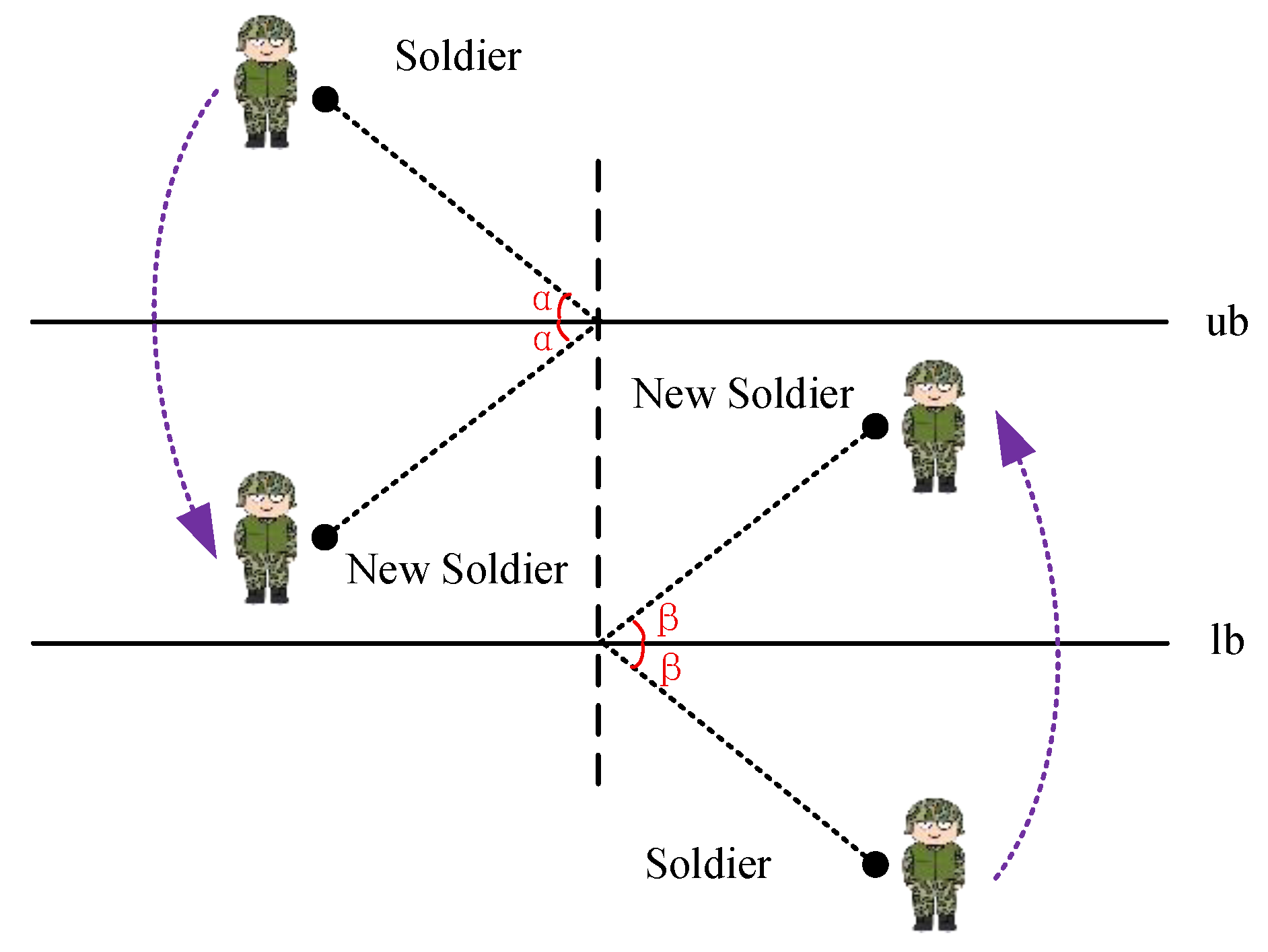
This mechanism strictly adheres to the geometric rule that the incident angle is equal to the reflection angle, bouncing the soldiers that are beyond the boundary back into the search space. The details are shown in Figure 6. Specifically, u b is the upper bound of the search space, and l b is the lower bound of the search space. Both α and β are the incident angle and the reflection angle. We can see that, if the soldier beyond the upper bound of the search space, this solider will be bounced back to the search space. Similarly, if the soldier is beyond the lower bound of the search space, this solider will be bounced back to the search space too.
S j , d t + 1 = 2 × l b S j , d t , i f S j , d t < l b 2 × u b S j , d t , i f S j , d t > u b
where S j , d t + 1 is the j t h soldier of the d t h dimension with ( t + 1 ) t h iteration, l b and u b are the lower and upper bounds of the search space, and S j , d t is the j t h soldier of the d t h dimension with t t h iteration.

3.4. TTBCA+: An Enhanced Besiege and Conquer Algorithm with Three-Three Tactics and Collision Theory

During the iterative process, the core is to generate the approach of soldiers. However, in BCA, the way soldiers surround the enemy is simple and irregular. This wastes a lot of soldiers and search time, which may cause the algorithm to deviate from the optimal solution.
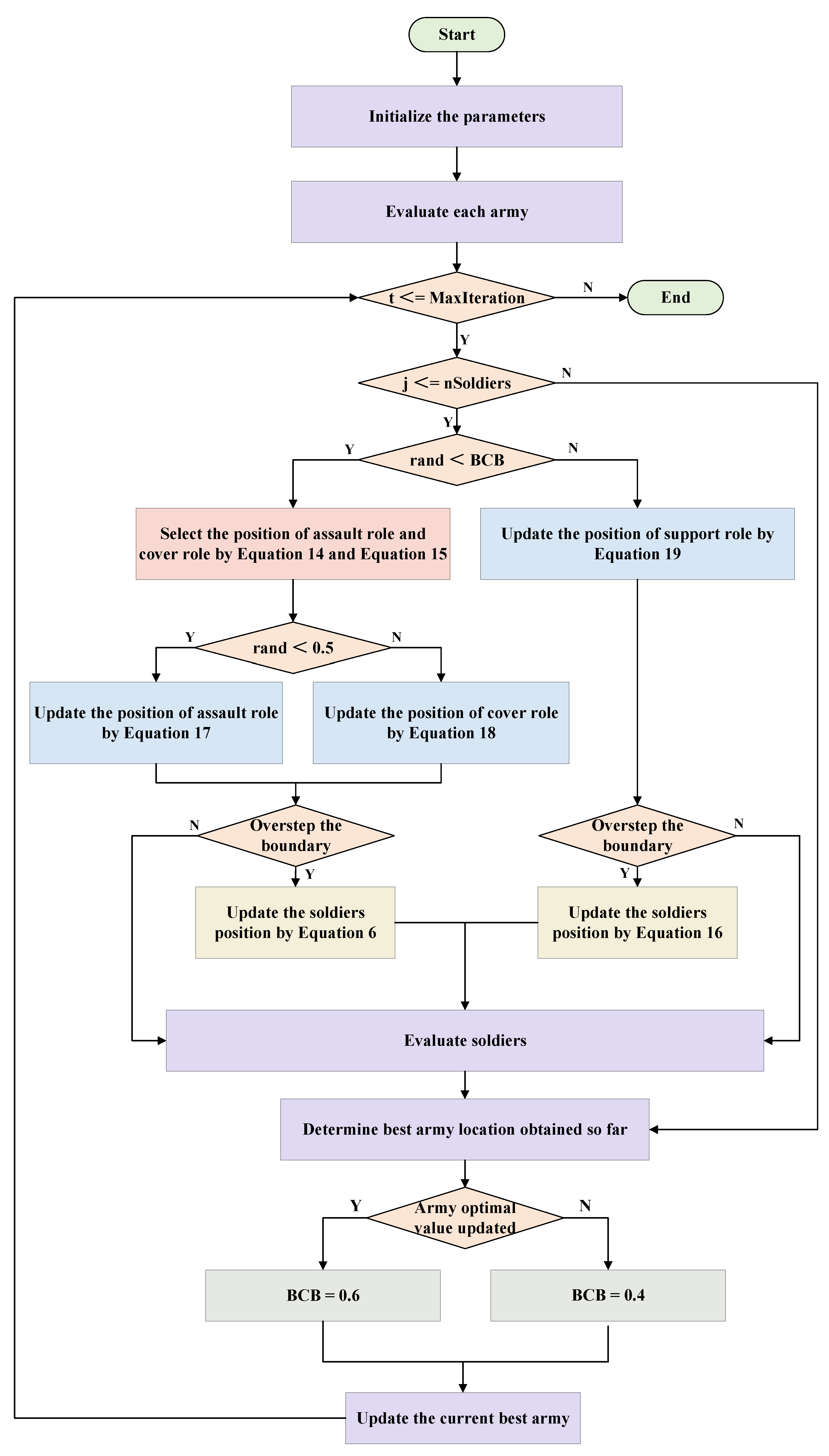
Therefore, this paper proposes three formulas to generate soldiers. Equation (17) is used to generate the assault role on the front. Equation (18) is used to generate the cover role on the front. Equation (19) is used to generate the support role on the battlefield.
S j , d t + 1 = R × A s l t P o s t d t + ( 1 R ) × B d t
S j , d t + 1 = C o v P o s t d t + ( C o v P o s t d t B d t ) × r a n d
S j , d t + 1 = A r , d t + | A r , d t A i , d t | × cos ( 2 × π × r a n d )
where R is in the rand of (0,1).
After the above methods, we finally propose TTBCA+. The working diagram of TTBCA+ can be summarized as Figure 7. The flow chart of TTBCA+ is shown in Figure 8. The pseudo-code of TTBCA+ is shown in Algorithm 1.
Figure 7. Working diagram of TTBCA+.
Electronics 14 04051 g007
Figure 8. The flow chart of TTBCA+.
Electronics 14 04051 g008
Algorithm 1. TTBCA+: an enhanced besiege and conquer algorithm with three-three tactics and collision theory
1:
Initialize the population N;
2:
Initialize the dimension of the problem D;
3:
Initialize the balance factor B C B ;
4:
Initialize the number of armies n A r m i e s ;
5:
Initialize the number of soldiers n S o l d i e r s ;
6:
Initialize the upper and lower bound u b , l b ;
7:
Configure the stopping criteria M a x _ I t e r a t i o n ;
8:
Initialize the army position through Equation (1);
9:
Evaluate all the soldiers;
10:
while  t < M a x _ I t e r a t i o n  do
11:
    for  i : n A r m i e s  do
12:
        Randomly select an army as the neighbor;
13:
        for  j : n S o l d i e r s  do
14:
           for  d : D  do
15:
               if  rand B C B  then
16:
                   Select the position of the assault soldiers by Equation (14);
17:
                   Select the position of the cover soldiers by Equation (15);
18:
                   if  rand 0 . 5  then
19:
                       Update the position of the i t h soldier by Equation (17);
20:
                       if  S j , d > u b | | S j , d < l b  then
21:
                          Update the position of the i t h soldier by Equation (6);
22:
                       end if
23:
                   else
24:
                       Update the position of the i t h soldier by Equation (18);
25:
                       if  S j , d > u b | | S j , d < l b  then
26:
                          Update the position of the i t h soldier by Equation (6);
27:
                       end if
28:
                   end if
29:
               else
30:
                   Update the position of the i t h soldier by Equation (19);
31:
                   if  S j , d > u b | | S j , d < l b  then
32:
                       Update the position of the i t h soldier by Equation (16);
33:
                   end if
34:
               end if
35:
           end for
36:
        end for
37:
    end for
38:
    Evaluate all the soldiers;
39:
end while
40:
Determine the best army location obtained so far;
41:
Judge whether the army optimal value is updated;
42:
if army optimal value is not updated then
43:
     B C B ( t + 1 ) = 0 . 4 ;
44:
else
45:
     B C B ( t + 1 ) = 0 . 6 ;
46:
end if
47:
Update the best army.

3.5. Dimension Rotation Mechanism

After the discussion and analysis in the above subsections, it is obvious that the proposed theory improvement BCA holds in the two-dimensional search space. This subsection discusses the definition of the three-three tactics search range in the high-dimensional search space.
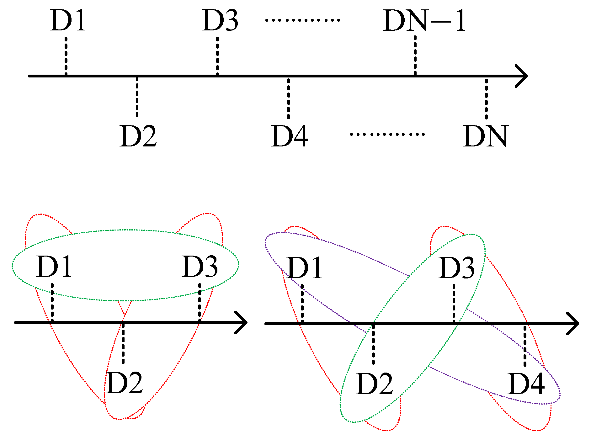
In the n-dimensional search space ( D i m e n s i o n N , D N ), the dimensional rotation mechanism ensures a comprehensive and efficient search process by arranging and combining different dimensional sub-spaces, avoiding omissions or generating a large number of repetitive searches. As shown in Figure 9, starting from the three-dimensional space, we select the combination of key dimensions and cycle the high-dimensional search space into multiple two-dimensional search space stages. For example, the three-dimensional space is cycled into three stages: D 1 & D 2 , D 2 & D 3 , D 3 & D 1 ; the four-dimensional space is cycled into four stages: D 1 & D 2 , D 3 & D 4 , D 4 & D 1 , D 2 & D 3 , and so on.

3.6. Computational Complexity Analysis

This section analyzes the computational complexity of the proposed algorithm from two aspects: time complexity analysis and space complexity analysis. During the analysis process, the maximum number of iterations T, population size N, problem dimension D, and fitness function f are defined.

3.6.1. Time Complexity Analysis

The initialization stage and fitness evaluation stage of the TTBCA+ are the same as BCA. Their time complexity analysis are T 1 = O ( N × D ) and T 2 = O ( N × D × f ( D ) ) , respectively. Therefore, the iterative stages that generate differences are mainly analyzed.
For TTBCA+, firstly, to generate a three-layer encirclement structure through three-three position deployment mechanism of soldiers, the search space needs to be traversed for each layer of reference points, with the time complexity being T 3 a = O ( 3 × T × D ) . Secondly, the division of roles among soldiers needs to be updated, with the time complexity being T 3 b = O ( 3 × ( N / 3 × T × D ) ) = O ( N × T × D ) . Thirdly, we adjust based on the update status of the optimal solution, with the time complexity being T 3 c = O ( T ) . Thus, the time complexity of the iteration stage is T 3 = T 3 a + T 3 b + T 3 c = O ( N × T × D ) . Finally, the time complexity of updating the global optimal solution in each iteration is T 4 = O ( T ) . To sum up, the time complexity of TTBCA+ is T = T 1 + T 2 + T 3 + T 4 = O ( N × T × ( D + f ( D ) ) ) .
It can be seen that these mechanisms increase the complexity of operations to a linear order and does not change the overall order of magnitude. Therefore, the time complexity of TTBCA+ is as same as BCA, and the execution efficiency of TTBCA+ will not significantly decrease due to the addition of these mechanisms.

3.6.2. Space Complexity Analysis

Space complexity refers to the measure of the amount of storage space temporarily occupied during the operation of an algorithm. The space complexity of TTBCA+ is mainly occupied by the following data structures:
Firstly, when initializing the population, the position information of N dimensional soldiers is generated, and the space complexity S 1 = O ( N × D ) is required for storage. Secondly, the space complexity S 2 = O ( N + D ) is required for recording the soldier roles and BCB. Finally, we store the space complexity S 3 = O ( 3 × D × T ) required for three-three position deployment mechanism of soldiers. To sum up, the space complexity of TTBCA is S = S 1 + S 2 + S 3 = O ( N × D ) .
Therefore, the space complexity of all mechanisms introduced by TTBCA+ is of linear order, which is consistent with the order of magnitude of the space complexity of BCA, and there is no significant increase in the demand for storage resources.

4. Results

To further evaluate the performance of the proposed algorithm, it is compared with 13 swarm intelligence algorithms, including BCA [12], JADE [13], lshade_rsp [14], AGWO [15], HOA [16], PLO [17], CFOA [18], HLOA [19], DBO [20], BOA [21], PSO [2], ABC [3], and GWO [22].

4.1. Experimental Settings

The experiments are coded on Matlab. As is customary, this paper selects the latest benchmark experimental environments IEEE CEC 2017 and IEEE CEC 2022, which attach importance to complex optimization problems, such as multimodal problems and composition problems, to verify the performance of TTBCA+.
IEEE CEC 2017 has 29 functions for solving minimum values. As shown in Table 1, F1–F2 are unimodal functions, F3–F9 are simple multimodal functions, F10–F19 are hybrid functions, and F20–F29 are composition functions. IEEE CEC 2022 has 12 functions for solving minimum values. F i * is the theoretical minimum value of the function F i at the global optimal solution X * . The more iterations an algorithm has, the closer it gets to the value X * . In this paper, the iteration is set to 100. As shown in Table 2, F1 is a unimodal function, F2–F5 are basic functions, F6–F8 are hybrid functions, and F9–F12 are composition functions.
All algorithms are run for 30 times to ensure the accuracy of statistical information. Meanwhile, we initialize BCB of TTBCA+ to 0.6 based on experimental rule of thumb, setting the search space dimension to 30 dimensions, 50 dimensions, and 100 dimensions, respectively, at IEEE CEC 2017 and to 10 dimensions and 20 dimensions, respectively, at IEEE CEC 2022, with the key parameters of other comparison algorithms remaining unchanged. The details of the initial parameters of comparative algorithms are shown in Table 3.

4.2. Test the Influence of the Four Innovations

This subsection uses 29 benchmark functions from IEEE CEC 2017 on 30 dimensions, 50 dimensions, and 100 dimensions to test the effect of TTBCA+.
Table 4 presents the average values of TTBCA+ and BCA on 29 benchmark functions at IEEE CEC 2017 on 30 dimensions, 50 dimensions, 100 dimensions, and the optimal solution is bolded. From the results, we can draw the following conclusions: compared with BCA, 28 functions ranked first on 30 dimensions, 29 functions ranked first on 50 dimensions, and 29 functions ranked first on 100 dimensions. This shows that TTBCA+ has been greatly improved in many benchmark functions, and our improvement of the algorithm is effective.
Table 1. The summary of IEEE CEC 2017.
No.Functions F i * = F i ( X * )
F1Shifted and Rotated Bent Cigar Function100
F2Shifted and Rotated Zakharov Function200
F3Shifted and Rotated Rosenbrock’s Function300
F4Shifted and Rotated Rastrigin’s Function400
F5Shifted and Rotated Expanded Schaffer’s f6 Function500
F6Shifted and Rotated Lunacek Bi_Rastrigin Function600
F7Shifted and Rotated Non-Continuous Rastrigin’s Function700
F8Shifted and Rotated Levy Function800
F9Shifted and Rotated Schwefel’s Function900
F10Hybrid Function 1 (N = 3)1000
F11Hybrid Function 2 (N = 3)1100
F12Hybrid Function 3 (N = 3)1200
F13Hybrid Function 4 (N = 4)1300
F14Hybrid Function 5 (N = 4)1400
F15Hybrid Function 6 (N = 4)1500
F16Hybrid Function 6 (N = 5)1600
F17Hybrid Function 6 (N = 5)1700
F18Hybrid Function 6 (N = 5)1800
F19Hybrid Function 6 (N = 6)1900
F20Composition Function 1 (N = 3)2000
F21Composition Function 2 (N = 3)2100
F22Composition Function 3 (N = 4)2200
F23Composition Function 4 (N = 4)2300
F24Composition Function 5 (N = 5)2400
F25Composition Function 6 (N = 5)2500
F26Composition Function 7 (N = 6)2600
F27Composition Function 8 (N = 6)2700
F28Composition Function 9 (N = 3)2800
F29Composition Function 10 (N = 3)2900
Table 2. The summary of IEEE CEC 2022.
No.Functions F i * = F i ( X * )
F1Shifted and Rotated Zakharov Function300
F2Shifted and Rotated Rosenbrock’s Function400
F3Shifted and Rotated Expanded Schaffer’s f6 Function600
F4Shifted and Rotated Non-Continuous Rastrigin’s Function800
F5Shifted and Rotated Levy Function900
F6Hybrid Function 1 (N = 3)1800
F7Hybrid Function 2 (N = 6)2000
F8Hybrid Function 3 (N = 5)2200
F9Composition Function 1 (N = 5)2300
F10Composition Function 2 (N = 4)2400
F11Composition Function 3 (N = 5)2600
F12Composition Function 4 (N = 6)2700
Table 3. The initial parameters of comparative algorithms.
AlgorithmParametersValues
TTBCA+ B C B 0.6
BCA B C B 0.8
JADE C R , F0.5, 0.5
lshade_rspp, H0.11, 5
AGWOafrom 2 to 0
PSO A c c e l e r a t i o n c o n s t a n t s 2
ABC S N , N P N P = 2 × S N
GWOafrom 2 to 0
HOA S F 1 or 2
PLO M u t a t i o n p r o b a b i l i t y 0.05
CFOA f m i n , f m a x 0, 10
HLOA a l p h a M e l a n o p h o r e 0.3
DBO P r o d u c e r s 0.2
BOAP0.8
Table 4. Comparisons between TTBCA+ and BCA at IEEE CEC 2017 on different dimensions.
D = 30D = 50D = 100
No.TTBCA+BCATTBCA+BCATTBCA+BCA
F1 4.2254 × 10 6 4.5965 × 10 10 6.1973 × 10 8 1.1161 × 10 11 2.2833 × 10 10 3.0803 × 10 11
F2 1.5486 × 10 5 2.0093 × 10 5 3.3522 × 10 5 3.6073 × 10 5 7.7968 × 10 5 8.5623 × 10 5
F3 5.4359 × 10 2 1.3317 × 10 4 8.3603 × 10 2 3.3138 × 10 4 3.7237 × 10 3 9.5170 × 10 4
F4 6.5656 × 10 2 8.1487 × 10 2 9.0363 × 10 2 1.1210 × 10 3 1.7786 × 10 3 2.1351 × 10 3
F5 6.1288 × 10 2 6.5597 × 10 2 6.2480 × 10 2 6.7685 × 10 2 6.5788 × 10 2 6.9617 × 10 2
F6 1.0251 × 10 3 1.8324 × 10 3 1.4333 × 10 3 3.1617 × 10 3 3.1125 × 10 3 7.4301 × 10 3
F7 9.6156 × 10 2 1.0755 × 10 3 1.2498 × 10 3 1.4618 × 10 3 2.1026 × 10 3 2.5311 × 10 3
F8 3.9228 × 10 3 1.0006 × 10 4 1.6894 × 10 4 3.8904 × 10 4 7.2683 × 10 4 1.0933 × 10 5
F9 8.1894 × 10 3 8.2115 × 10 3 1.4328 × 10 4 1.6729 × 10 4 2.6801 × 10 4 3.0012 × 10 4
F10 1.4641 × 10 3 1.5161 × 10 4 5.1860 × 10 3 3.6695 × 10 4 2.7047 × 10 5 3.3991 × 10 5
F11 3.6943 × 10 6 6.7390 × 10 9 5.5154 × 10 7 3.7518 × 10 10 1.6705 × 10 9 1.3761 × 10 11
F12 8.6683 × 10 4 6.6019 × 10 9 1.6390 × 10 5 2.8003 × 10 10 2.0933 × 10 6 3.4785 × 10 10
F13 6.8666 × 10 5 5.7990 × 10 6 2.3661 × 10 6 4.9787 × 10 7 1.1855 × 10 7 1.0989 × 10 8
F14 1.3688 × 10 8 1.2757 × 10 9 3.5119 × 10 4 6.3910 × 10 9 1.7175 × 10 5 1.3836 × 10 10
F15 2.9866 × 10 3 4.5970 × 10 3 4.1329 × 10 3 6.8138 × 10 3 1.1059 × 10 4 1.4688 × 10 4
F16 2.2615 × 10 3 4.2707 × 10 3 3.6823 × 10 3 9.2769 × 10 4 6.7148 × 10 3 2.2337 × 10 6
F17 4.2714 × 10 6 3.1899 × 10 7 9.1087 × 10 6 1.8302 × 10 8 2.0001 × 10 7 1.4562 × 10 8
F18 1.1466 × 10 4 1.4769 × 10 9 3.4702 × 10 4 3.4454 × 10 9 6.7573 × 10 5 1.3769 × 10 10
F19 2.5494 × 10 3 2.8977 × 10 3 4.0409 × 10 3 4.1026 × 10 3 6.5523 × 10 3 8.7678 × 10 3
F20 2.4660 × 10 3 2.5995 × 10 3 2.7396 × 10 3 2.9461 × 10 3 3.6525 × 10 3 4.1670 × 10 3
F21 7.5183 × 10 3 7.3451 × 10 3 1.8619 × 10 4 1.9156 × 10 4 3.0921 × 10 4 3.3392 × 10 4
F22 2.8101 × 10 3 3.1517 × 10 3 3.1640 × 10 3 3.9557 × 10 3 3.8692 × 10 3 5.3263 × 10 3
F23 2.9753 × 10 3 3.3568 × 10 3 3.3674 × 10 3 4.0710 × 10 3 4.6864 × 10 3 7.7796 × 10 3
F24 2.9262 × 10 3 6.1435 × 10 3 3.3096 × 10 3 1.5541 × 10 4 6.5760 × 10 3 4.6676 × 10 4
F25 4.8919 × 10 3 9.2190 × 10 3 7.9653 × 10 3 1.5024 × 10 4 2.1173 × 10 4 3.9403 × 10 4
F26 3.2705 × 10 3 3.7567 × 10 3 3.6638 × 10 3 5.0410 × 10 3 3.9479 × 10 3 7.7809 × 10 3
F27 3.3221 × 10 3 6.4043 × 10 3 4.1301 × 10 3 1.1710 × 10 4 8.9635 × 10 3 3.2381 × 10 4
F28 4.0517 × 10 3 5.3483 × 10 3 4.5683 × 10 3 4.6937 × 10 4 8.9584 × 10 3 1.1039 × 10 6
F29 1.0090 × 10 5 4.9853 × 10 8 5.8166 × 10 6 5.0592 × 10 9 1.1897 × 10 7 2.6070 × 10 10

4.3. Compare the New Algorithm with Other Algorithms at IEEE CEC 2017

To further evaluate the performance of TTBCA+, this subsection compares it with 9 swarm intelligence algorithms at IEEE CEC 2017, including BCA, JADE, PSO, HOA, PLO, CFOA, HLOA, ABC, and lshade_rsp on 30 dimensions, 50 dimensions, and 100 dimensions. The results are shown in Table 5, Table 6 and Table 7.
From Table 5 to Table 7, compared with other algorithms, 20 functions ranked first on 30 dimensions, 20 functions ranked first on 50 dimensions, 16 functions ranked first on 100 dimensions. We can draw the conclusion: the optimization effect of TTBCA+ on the benchmark functions are better than other algorithms. This shows that we have achieved remarkable results in improving BCA.
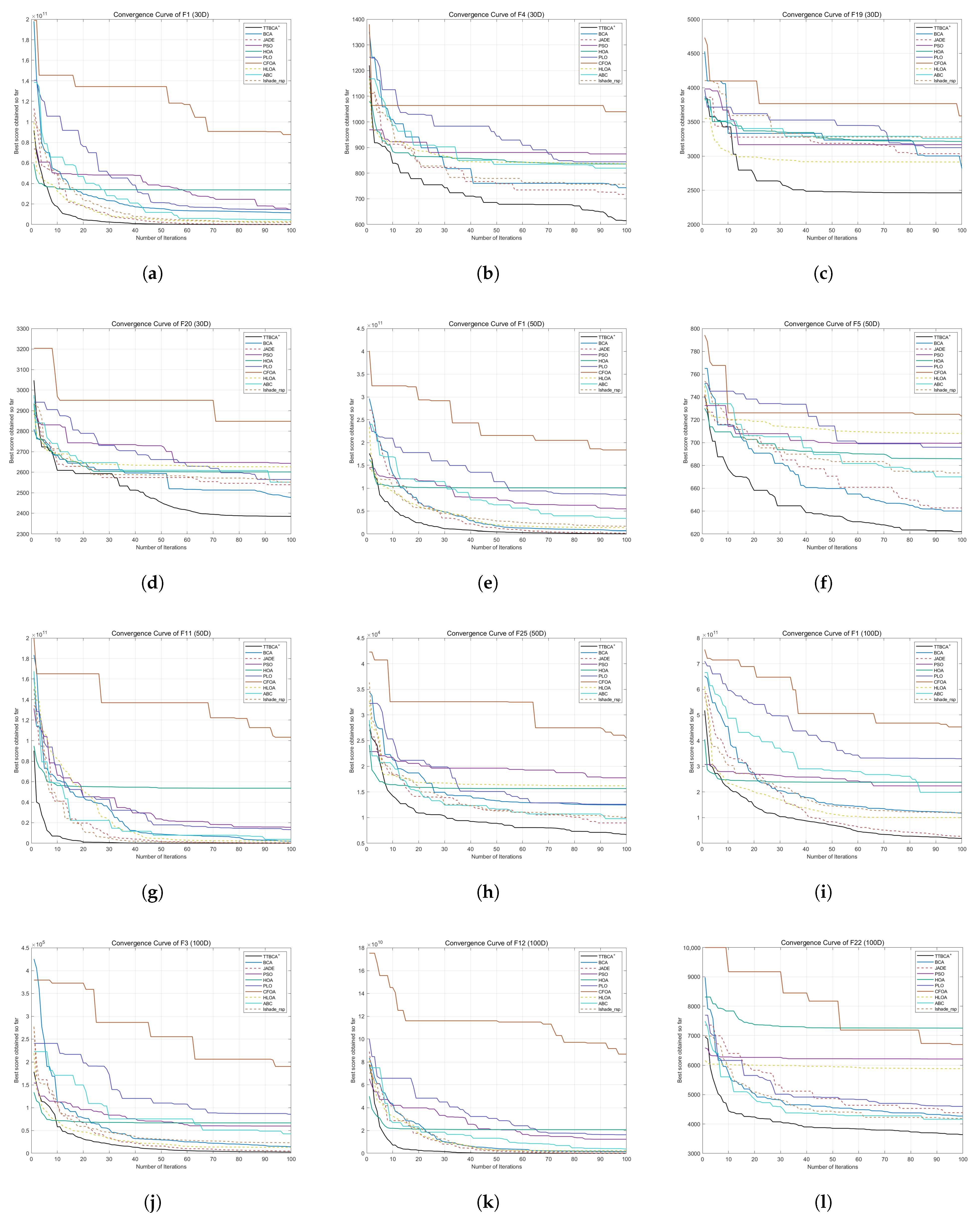
The convergence curve of the compared algorithms, like BCA, JADE, PSO, HOA, PLO, CFOA, HLOA, ABC, lshade_rsp of some functions on 30 dimensions, 50 dimensions, and 100 dimensions are reported in Figure 10.
These figures proved the convergence speed of TTBCA+ has been markedly enhanced, and the optimization capability of TTBCA+ has been significantly improved. This shows that our improvement are valuable and effective.

4.4. Compare the New Algorithm with Other Algorithms at IEEE CEC 2022

To further verify the performance and superiority of TTBCA+, it was compared with 10 swarm intelligence algorithms such as classical algorithm PSO, GWO, well-known improved algorithm AGWO, and latest algorithms BCA, HOA, DBO, PLO, CFOA, HLOA, and BOA at IEEE CEC 2022. This paper set the search space dimension to 10 dimensions and 20 dimensions. The results are shown in Table 8 and Table 9.
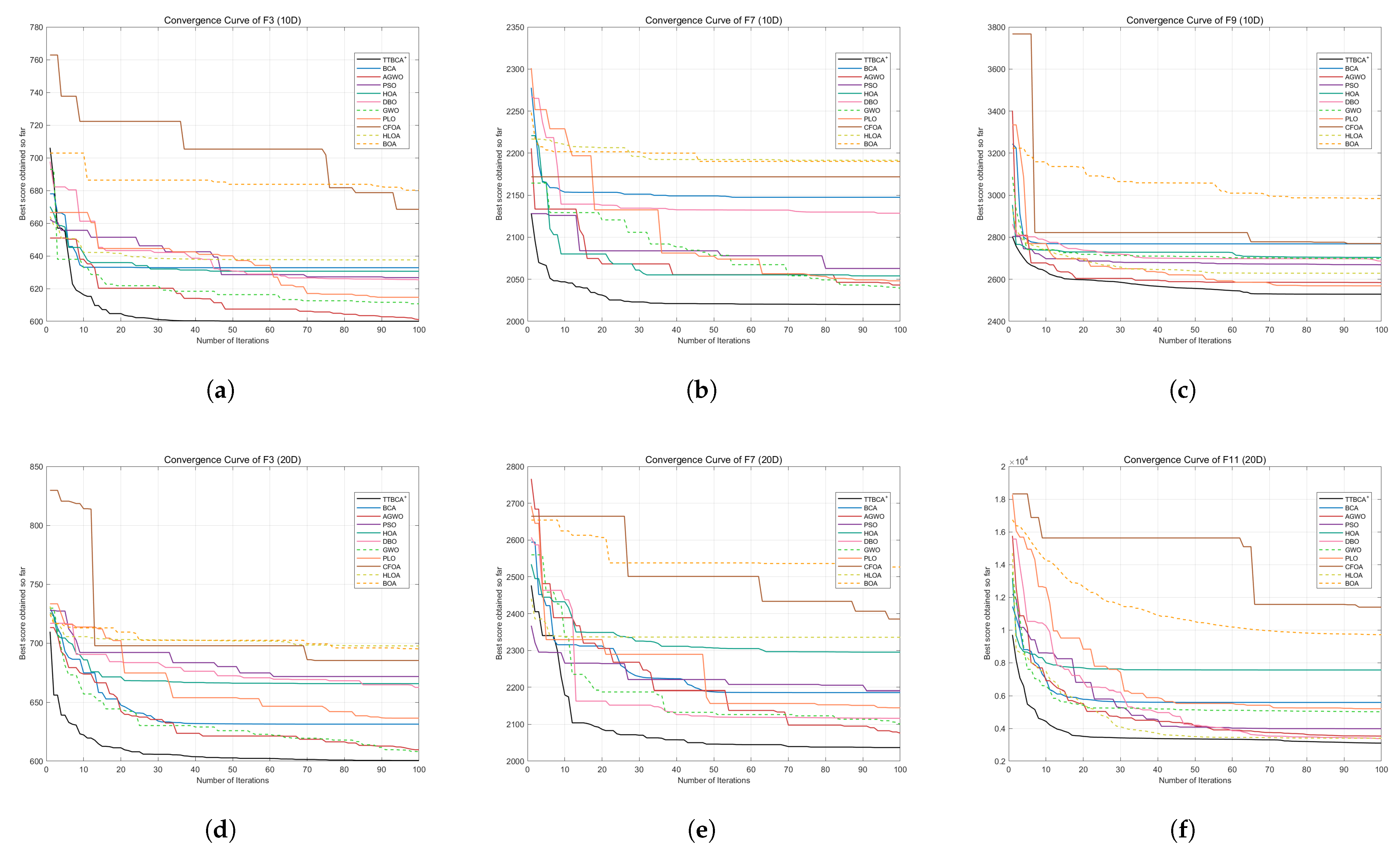
In addition, this study further plotted the convergence curve of some functions on 10 dimensions and 20 dimensions in Figure 11. It clearly shows the performance of TTBCA+ and other algorithms such as BCA, AGWO, PSO, HOA, DBO, GWO, PLO, CFOA, HLOA, and BOA throughout the entire process.
Through the detailed analysis of the results from Table 8 to Table 9, and in combination with the convergence curve in Figure 11, we can draw the following conclusion: TTBCA+ stood out among the 11 swarm intelligence algorithms tested with the performance of ranking first in 8 functions on 10 dimensions and 7 functions on 20 dimensions. It is proven that TTBCA+ can effectively balance exploration and exploitation, avoid getting itself trapped in local optimum too early, and perform well in complex functions. This proved that TTBCA+ can effectively improve the performance of BCA.

4.5. Ablation Experiment of TTBCA+

In order to verify the specific impact of the improved mechanisms introduced by the TTBCA+ on the overall performance of the algorithm, an ablation experiment was conducted in it at IEEE CEC 2017 on 30 dimensions, 50 dimensions, and 100 dimensions.
This subsection breaks down the four mechanisms of TTBCA+ and obtains four algorithms, referred to as TTBCA+1, TTBCA+2, TTBCA+3, and TTBCA+4. These algorithms adopt different mechanisms: TTBCA+1 improved by three-three allocation mechanism of battlefield and roles, TTBCA+2 improved by three-three position deployment mechanism of soldiers, TTBCA+3 modified the balance factor, and TTBCA+4 improved by collision mechanism. Table 10 shows detailed information on the changes of parameter or mechanism for TTBCA+1 to TTBCA+4. If the algorithm has this part of the content, it is represented by the symbol ✓; otherwise, it is represented by the symbol ×. Table 11, Table 12 and Table 13 show the average values of the ablation experiment.
As shown in Table 11, Table 12 and Table 13, in this ablation experiment, 16 functions of TTBCA+ ranked first in 30 dimensions, 17 functions ranked first in 50 dimensions, and 20 functions ranked first in 100 dimensions. The overall ranking of TTBCA+ is first, the reasons are as follows.
Firstly, three-three allocation mechanism of battlefield and roles improve the besiege strategy. Secondly, three-three position deployment mechanism of soldiers improves the conquer strategy to increase the capability to escape the local optimum, increasing the coverage capability of search space. Thirdly, we modified the balance factor BCB to improve the balance strategy. Finally, the collision mechanism bouncing the soldiers that cross the boundary back into the search space improves the continuity of the search process.
Based on the analysis of the comprehensive experimental results, the four innovative mechanisms of TTBCA+ are all indispensable. They have significantly improved the efficiency and stability of the algorithm, which can effectively solve the problems existing in BCA.

4.6. Statistical Experiments

To verify the superiority demonstrated by the TTBCA+, this subsection uses the experimental data from Section 4.3 and Section 4.4 to verify the results through the Wilcoxon Signed Rank Test. Table 14, Table 15, Table 16, Table 17 and Table 18 present the p-values of the Wilcoxon Signed Rank Test applied to the experimental data of TTBCA+ at IEEE CEC 2017 on 30 dimensions, 50 dimensions, and 100 dimensions and at IEEE CEC 2022 on 10 dimensions and 20 dimensions respectively.
When the p-value is less than the significance level of 0.05, it indicates that the test results reject the hypothesis, that is, TTBCA+ performs better. Specifically, in the last row of Table 14, Table 15, Table 16, Table 17 and Table 18, the symbol + represents the number of benchmark functions in which the performance of TTBCA+ is better than this comparison algorithm, and the symbol − represents the number of benchmark functions in which the performance of TTBCA+ is worse than this comparison algorithm.
It can be seen in Table 14, Table 15, Table 16, Table 17 and Table 18, compared with other algorithms, the results of the vast majority of the Wilcoxon Signed Rank Test of TTBCA+ satisfy the p-value less than 0.05. This indicates that from a statistical point of view, the optimization capability of TTBCA+ is superior to other algorithms, which proved the improvement of TTBCA+ is effective.

5. Application of TTBCA+ in Engineering Design Problems

This section further verifies the performance and efficiency of TTBCA+ by solving two constrained real engineering design problems: multiple disk clutch brake design problem [23] and three-bar truss design problem [24]. These problems have been widely discussed in the literature and well resolved, which can fully illustrate the effectiveness of the algorithm.

5.1. Multiple Disk Clutch Brake Design Problem

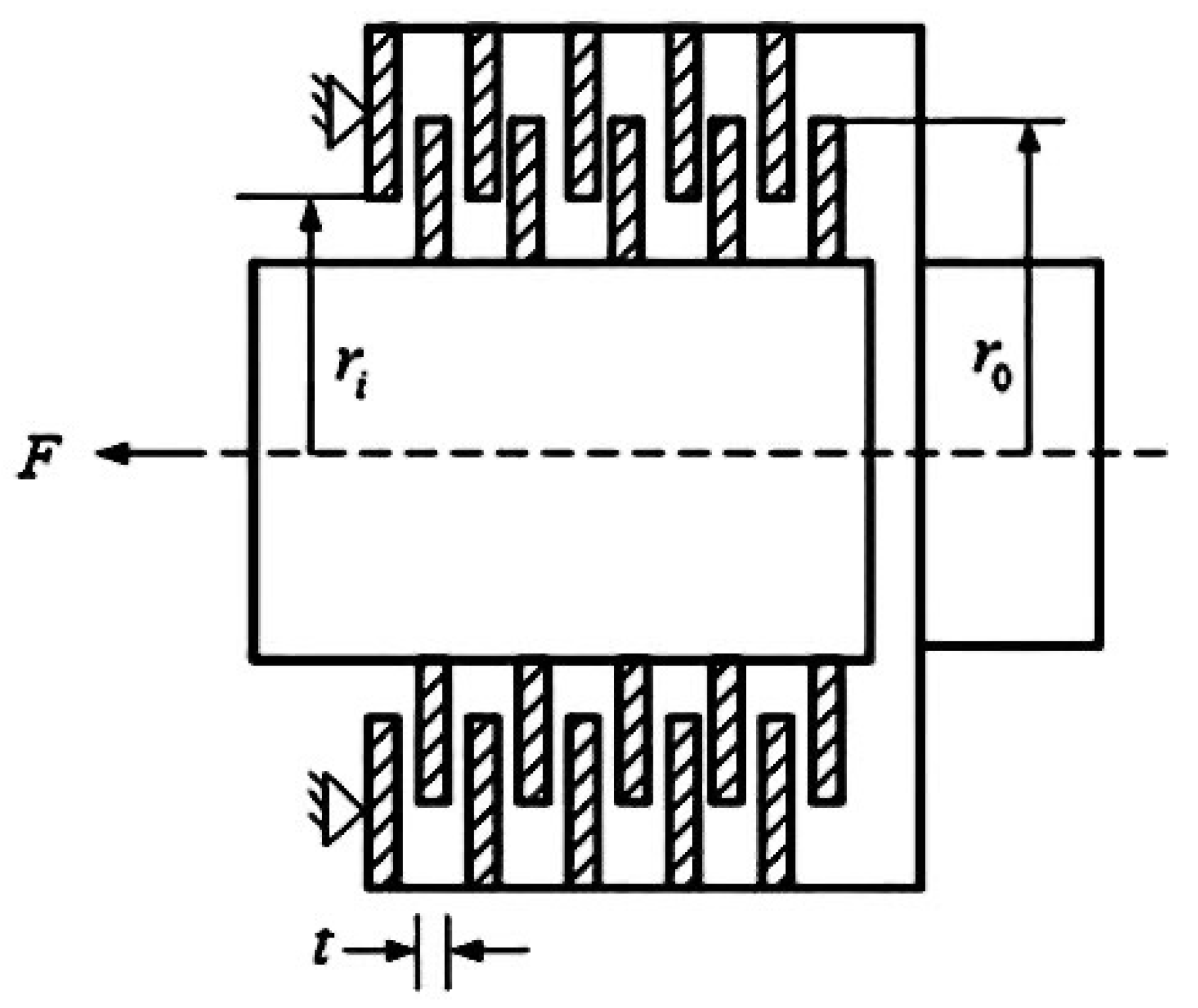
The aim of this engineering problem is to minimize the mass of multiple disk clutch brake as much as possible. This problem mainly includes five decision variables: inner radius ( r i ), outer radius ( r 0 ), disk thickness (t), action force (F), and the number of friction surfaces (Z). The schematic diagram of this problem is presented in Figure 12. Table 19 gives the detailed mathematical formulations of multiple disk clutch brake design problem.
In order to verify the performance of TTBCA+ in the multiple disk clutch brake design problem, this paper compares it with HHO [25], GWO [22], SO [26], DO [27], and BWO [28]. The results are shown in Table 20. It can be seen that TTBCA+ has achieved the best results in this problem and has a relatively short operating time.

5.2. Three-Bar Truss Design Problem

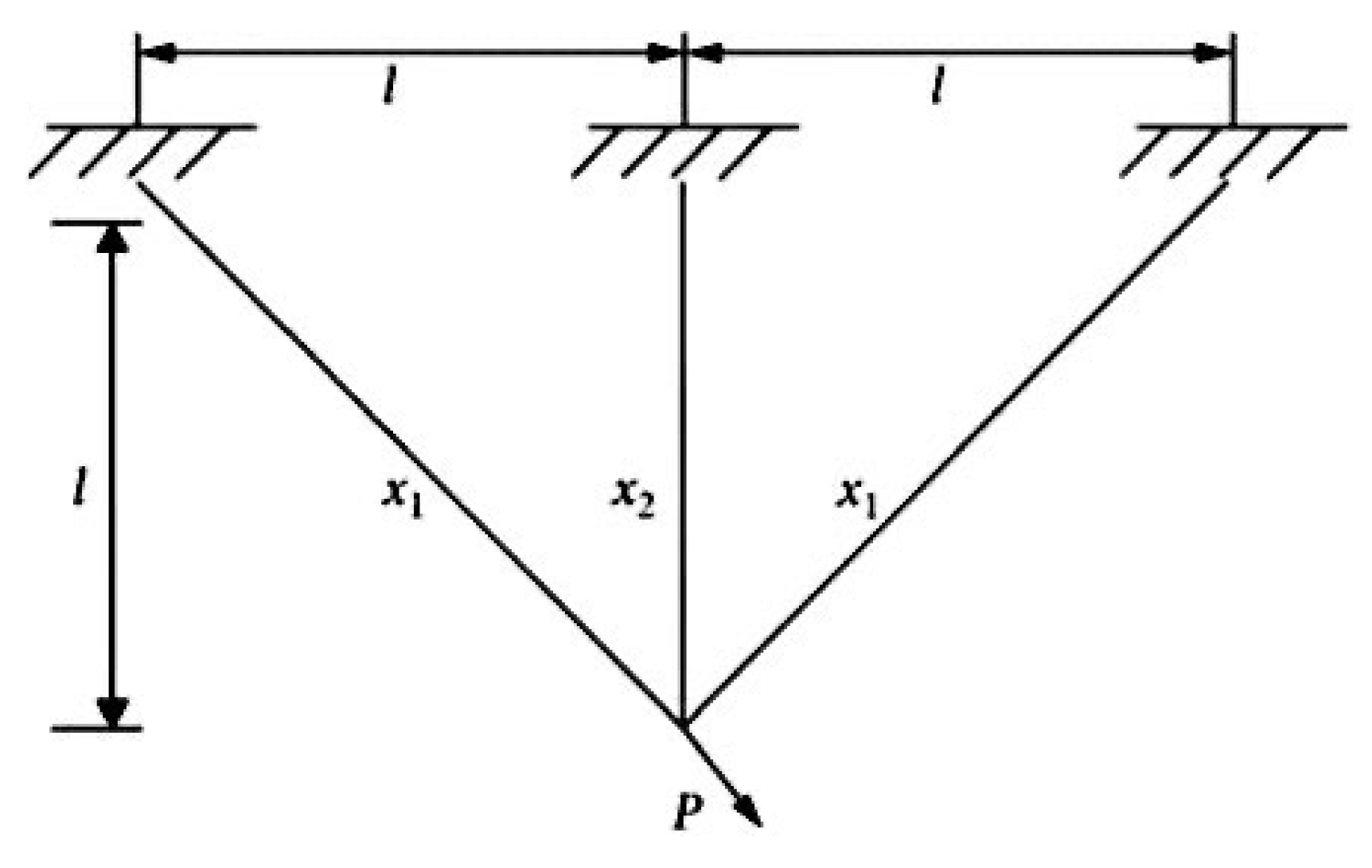
The main objective of this engineering problem is to minimize the total weight of the structure by controlling two parameters: the cross-sectional areas X 1 and X 2 . The schematic diagram of this problem is presented in Figure 13. Table 21 gives the detailed mathematical formulations of three-bar truss design problem.
In order to fully verify the performance of TTBCA+ in the three-bar truss design problem, this paper compares it with BCA [12], SMA [29], RIME [30], CFOA [18], and PSA [31]. As shown in Table 22, TTBCA+ has achieved the best results in this problem.

6. Discussion and Conclusions

BCA has four problems in solving complex optimization problems. First, the besiege strategy of soldiers lacks diversity. Second, the conquer strategy leads to the solution being prone to getting stuck in local optima. Third, repeated searches of a certain area result in the waste of soldiers’ resources. Fourth, the way of regenerating the soldiers that cross the boundary disrupted the continuity of the search process. To overcome these challenges, this paper introduces three-three allocation mechanism of battlefield and roles, three-three position deployment mechanism of soldiers, and modified balance parameter BCB and collision mechanism to improve BCA.
  • The proposed three-three allocation mechanism of battlefield and roles has a strict division, naturally achieving the diversity of search mode.
  • The proposed three-three position deployment mechanism of soldiers improved local search capability of BCA and reduce the waste of resources.
  • The modification of BCB is more beneficial for balancing exploration and exploitation.
  • The proposed collision mechanism improves the continuity of the search process.
Based on the analysis and discussion of the results of a large number of experiments, we can conclude that TTBCA+ ranked first in 63.96% of the benchmark functions in comparative experiments at IEEE CEC 2017 and IEEE CEC 2022. In addition, through statistical experiments, a large number of the Wilcoxon Signed Rank Test of TTBCA+ satisfy the p-value less than 0.05. These results show that the performance of TTBCA+ is highly competitive. It is hoped that the four improvement methods proposed in this article will have a profound impact on swarm intelligence algorithms. In the future, TTBCA+ can further combine with other tactics to enhance its local search capability. What is more, we will improve the overly average search method for specific areas to enhance its global search capability.

Author Contributions

Conceptualization, J.J. and X.X.; methodology, J.J.; software, X.X.; validation, X.X., J.T. and H.L.; formal analysis, X.X.; writing—original draft preparation, X.X.; writing—review and editing, J.J.; funding acquisition, J.J. All authors have read and agreed to the published version of the manuscript.

Funding

This work was supported by the Foundation of the Jilin Provincial Department of Science and Technology No. YDZJ202201ZYTS565.

Data Availability Statement

The original contributions presented in the study are included in the article. Further inquiries can be directed to the corresponding author.

Conflicts of Interest

The authors declare no conflicts of interest.

References

  1. Chakraborty, A.; Kar, A.K. Swarm intelligence: A review of algorithms. In Nature-Inspired Computing and Optimization: Theory and Applications; Springer: Cham, Switzerland, 2017; pp. 475–494. [Google Scholar]
  2. Kennedy, J.; Eberhart, R. Particle swarm optimization. In Proceedings of the ICNN’95-International Conference on Neural Networks, Perth, WA, Australia, 27 November–1 December 1995; Volume 4, pp. 1942–1948. [Google Scholar]
  3. Karaboga, D.; Basturk, B. A powerful and efficient algorithm for numerical function optimization: Artificial bee colony (ABC) algorithm. J. Glob. Optim. 2007, 39, 459–471. [Google Scholar] [CrossRef]
  4. Kiran, M.S. TSA: Tree-seed algorithm for continuous optimization. Expert Syst. Appl. 2015, 42, 6686–6698. [Google Scholar] [CrossRef]
  5. Bai, L.; Pei, Z.; Wang, J.; Zhou, Y. Multi-Strategy Improved Aquila Optimizer Algorithm and Its Application in Railway Freight Volume Prediction. Electronics 2025, 14, 1621. [Google Scholar] [CrossRef]
  6. Dai, F.; Ma, T.; Gao, S. Optimal Design of a Fractional Order PIDD2 Controller for an AVR System Using Hybrid Black-Winged Kite Algorithm. Electronics 2025, 14, 2315. [Google Scholar] [CrossRef]
  7. Jiang, J.H.; Wu, J.Q.; Luo, J.M.; Yang, X.; Huang, Z.L. MOBCA: Multi-Objective Besiege and Conquer Algorithm. Biomimetics 2024, 9, 316. [Google Scholar] [CrossRef]
  8. Jiang, J.H.; Meng, X.Q.; Chen, Y.J.; Qiu, C.Y.; Liu, Y.; Li, K.Q. Enhancing tree-seed algorithm via feed-back mechanism for optimizing continuous problems. Appl. Soft Comput. 2020, 92, 106314. [Google Scholar] [CrossRef]
  9. Jiang, J.H.; Huang, J.S.; Wu, J.Q.; Luo, J.M.; Yang, X.; Li, W.H. DTSA: Dynamic Tree-Seed Algorithm with Velocity-Driven Seed Generation and Count-Based Adaptive Strategies. Symmetry 2024, 16, 795. [Google Scholar]
  10. Li, H.; Jiang, J.H.; Ma, Z.X.; Li, L.N.; Liu, J.Y.; Li, C.X.; Yu, Z.H. A Symmetry-Driven Adaptive Dual-Subpopulation Tree–Seed Algorithm for Complex Optimization with Local Optima Avoidance and Convergence Acceleration. Symmetry 2025, 17, 1200. [Google Scholar]
  11. Yang, X.S.; Deb, S.; Zhao, Y.X.; Fong, S.; He, X. Swarm intelligence: Past, present and future. Soft Comput. 2018, 22, 5923–5933. [Google Scholar]
  12. Jiang, J.H.; Meng, X.Q.; Wu, J.Q.; Tian, J.; Xu, G.C.; Li, W.H. BCA: Besiege and Conquer Algorithm. Symmetry 2025, 17, 217. [Google Scholar] [CrossRef]
  13. Zhang, J.; Sanderson, A.C. JADE: Adaptive differential evolution with optional external archive. IEEE Trans. Evol. Comput. 2009, 13, 945–958. [Google Scholar] [CrossRef]
  14. Vladimir, S.; Shakhnaz, A.; Eugene, S. LSHADE Algorithm with Rank-Based Selective Pressure Strategy for Solving CEC 2017 Benchmark Problems. In Proceedings of the 2018 IEEE Congress on Evolutionary Computation (CEC), Rio de Janeiro, Brazil, 8–13 July 2018; pp. 1–8. [Google Scholar]
  15. Meng, X.Q.; Jiang, J.H.; Wang, H. AGWO: Advanced GWO in multi-layer perception optimization. Expert Syst. Appl. 2021, 173, 114676. [Google Scholar] [CrossRef]
  16. Oladejo, S.O.; Ekwe, S.O.; Mirjalili, S. The Hiking Optimization Algorithm: A novel human-based metaheuristic approach. Knowl.-Based Syst. 2024, 296, 111880. [Google Scholar] [CrossRef]
  17. Yuan, C.; Zhao, D.; Heidari, A.A.; Liu, L.; Chen, Y.; Chen, H. Polar lights optimizer: Algorithm and applications in image segmentation and feature selection. Neurocomputing 2024, 607, 128427. [Google Scholar] [CrossRef]
  18. Jia, H.; Wen, Q.; Wang, Y.; Mirjalili, S. Catch fish optimization algorithm: A new human behavior algorithm for solving clustering problems. Clust. Comput. 2024, 27, 13295–13332. [Google Scholar] [CrossRef]
  19. Peraza-Vázquez, H.; Peña-Delgado, A.; Merino-Treviño, M.; Morales-Cepeda, A.B.; Sinha, N. A novel metaheuristic inspired by horned lizard defense tactics. Artif. Intell. Rev. 2024, 57, 59. [Google Scholar] [CrossRef]
  20. Xue, J.; Shen, B. Dung beetle optimizer: A new meta-heuristic algorithm for global optimization. J. Supercomput. 2023, 79, 7305–7336. [Google Scholar] [CrossRef]
  21. Sankalap, A.; Satvir, S. Butterfly optimization algorithm: A novel approach for global optimization. Soft Comput. 2019, 23, 715–734. [Google Scholar]
  22. Mirjalili, S.; Mirjalili, S.M.; Lewis, A. Grey wolf optimizer. Adv. Eng. Softw. 2014, 69, 46–61. [Google Scholar] [CrossRef]
  23. Rao, R.V.; Savsani, V.J.; Vakharia, D.P. Teaching–learning-based optimization: A novel method for constrained mechanical design optimization problems. Comput.-Aided Des. 2011, 43, 303–315. [Google Scholar] [CrossRef]
  24. Yildirim, A.E.; Karci, A. Application of three bar truss problem among engineering design optimization problems using artificial atom algorithm. In Proceedings of the 2018 International Conference on Artificial Intelligence and Data Processing, Malatya, Turkey, 28–30 September 2018; pp. 1–5. [Google Scholar]
  25. Heidari, A.A.; Mirjalili, S.; Faris, H.; Aljarah, I.; Mafarja, M.; Chen, H. Harris hawks optimization: Algorithm and applications. Future Gener. Comput. Syst. 2019, 97, 849–872. [Google Scholar]
  26. Hashim, F.A.; Hussien, A.G. Snake Optimizer: A novel meta-heuristic optimization algorithm. Knowl.-Based Syst. 2022, 242, 108320. [Google Scholar] [CrossRef]
  27. Zhao, S.; Zhang, T.; Ma, S.; Chen, M. Dandelion Optimizer: A nature-inspired metaheuristic algorithm for engineering applications. Eng. Appl. Artif. Intell. 2022, 114, 105075. [Google Scholar] [CrossRef]
  28. Zhong, C.; Li, G.; Meng, Z. Beluga whale optimization: A novel nature-inspired metaheuristic algorithm. Knowl.-Based Syst. 2022, 251, 109215. [Google Scholar] [CrossRef]
  29. Li, S.; Chen, H.; Wang, M.; Heidari, A.A.; Mirjalili, S. Slime mould algorithm: A new method for stochastic optimization. Future Gener. Comput. Syst. 2020, 111, 300–323. [Google Scholar] [CrossRef]
  30. Su, H.; Zhao, D.; Heidari, A.A.; Liu, L.; Zhang, X.; Mafarja, M.; Chen, H. RIME: A physics-based optimization. Neurocomputing 2023, 532, 183–214. [Google Scholar] [CrossRef]
  31. Gao, Y. PID-based search algorithm: A novel metaheuristic algorithm based on PID algorithm. Expert Syst. Appl. 2023, 232, 120886. [Google Scholar] [CrossRef]
Figure 1. Three-three allocation mechanism of battlefield and roles.
Electronics 14 04051 g001
Figure 2. The reference points of first layer generation.
Electronics 14 04051 g002
Figure 3. The reference points of second layer generation.
Electronics 14 04051 g003
Figure 4. The reference points of third layer generation.
Electronics 14 04051 g004
Figure 5. Three-three position deployment mechanism of soldiers.
Electronics 14 04051 g005
Figure 6. Collision mechanism.
Electronics 14 04051 g006
Figure 9. Dimension rotation mechanism.
Electronics 14 04051 g009
Figure 10. Convergence curve of TTBCA+, BCA, JADE, PSO, HOA, PLO, CFOA, HLOA, ABC, and lshade_rsp of some functions on 30 dimensions, 50 dimensions, and 100 dimensions. (a) F1 convergence curve on 30 dimensions. (b) F4 convergence curve on 30 dimensions. (c) F19 convergence curve on 30 dimensions. (d) F20 convergence curve on 30 dimensions. (e) F1 convergence curve on 50 dimensions. (f) F5 convergence curve on 50 dimensions. (g) F11 convergence curve on 50 dimensions. (h) F25 convergence curve on 50 dimensions. (i) F1 convergence curve on 100 dimensions. (j) F3 convergence curve on 100 dimensions. (k) F12 convergence curve on 100 dimensions. (l) F22 convergence curve on 100 dimensions.
Electronics 14 04051 g010
Figure 11. Convergence curve of TTBCA+, BCA, AGWO, PSO, HOA, DBO, GWO, PLO, CFOA, HLOA, and BOA of some functions on 10 dimensions and 20 dimensions. (a) F3 convergence curve on 10 dimensions. (b) F7 convergence curve on 10 dimensions. (c) F9 convergence curve on 10 dimensions. (d) F3 convergence curve on 20 dimensions. (e) F7 convergence curve on 20 dimensions. (f) F11 convergence curve on 20 dimensions.
Electronics 14 04051 g011
Figure 12. Multiple disk clutch brake design problem schematic.
Electronics 14 04051 g012
Figure 13. Three-bar truss design problem schematic.
Electronics 14 04051 g013
Table 5. Comparisons between TTBCA+ and other algorithms on 30 dimensions.
No.TTBCA+BCAJADEPSOHOAPLOCFOAHLOAABClshade_rsp
F1 4.1101 × 10 6 4.8370 × 10 9 5.5751 × 10 7 1.7852 × 10 10 3.6439 × 10 10 2.1546 × 10 10 9.0170 × 10 10 2.9689 × 10 9 4.5174 × 10 9 2.4848 × 10 9
F2 1.6941 × 10 5 2.1651 × 10 5 1.1685 × 10 5 2.6362 × 10 5 8.0818 × 10 4 1.6628 × 10 5 1.3120 × 10 6 7.7848 × 10 4 1.9501 × 10 5 6.9576 × 10 4
F3 5.3984 × 10 2 1.8943 × 10 3 5.5332 × 10 2 2.9454 × 10 3 7.0500 × 10 3 3.0233 × 10 3 3.1370 × 10 4 9.5289 × 10 2 1.2387 × 10 3 7.5711 × 10 2
F4 6.6806 × 10 2 7.4114 × 10 2 7.4382 × 10 2 8.5966 × 10 2 8.1941 × 10 2 8.2400 × 10 2 1.0607 × 10 3 8.4393 × 10 2 7.9493 × 10 2 7.5816 × 10 2
F5 6.1266 × 10 2 6.1871 × 10 2 6.1647 × 10 2 6.7562 × 10 2 6.6799 × 10 2 6.6779 × 10 2 7.2186 × 10 2 6.8764 × 10 2 6.3556 × 10 2 6.3498 × 10 2
F6 9.8939 × 10 2 1.1232 × 10 3 9.9462 × 10 2 1.3723 × 10 3 1.2430 × 10 3 1.5714 × 10 3 2.3372 × 10 3 1.3935 × 10 3 1.1609 × 10 3 1.0752 × 10 3
F7 9.6997 × 10 2 1.0120 × 10 3 1.0337 × 10 3 1.1440 × 10 3 1.0627 × 10 3 1.1065 × 10 3 1.3020 × 10 3 1.0771 × 10 3 1.0929 × 10 3 1.0443 × 10 3
F8 4.0128 × 10 3 5.4643 × 10 3 2.5803 × 10 3 1.3670 × 10 4 8.4867 × 10 3 1.3475 × 10 4 2.8793 × 10 4 9.4536 × 10 3 9.1401 × 10 3 4.4975 × 10 3
F9 8.3799 × 10 3 8.9699 × 10 3 8.8850 × 10 3 8.7042 × 10 3 7.8576 × 10 3 7.8440 × 10 3 1.0227 × 10 4 7.4356 × 10 3 9.0949 × 10 3 9.2146 × 10 3
F10 1.6142 × 10 3 3.8962 × 10 3 2.0226 × 10 3 1.0419 × 10 4 6.2536 × 10 3 1.0592 × 10 4 3.4834 × 10 4 3.5462 × 10 3 8.1240 × 10 3 1.6727 × 10 3
F11 3.2377 × 10 6 1.6178 × 10 8 8.8543 × 10 6 1.6128 × 10 9 7.2314 × 10 9 1.3200 × 10 9 1.7249 × 10 10 3.5764 × 10 8 2.4088 × 10 8 3.4377 × 10 7
F12 5.2527 × 10 4 9.0500 × 10 6 1.2237 × 10 6 9.6502 × 10 8 2.0220 × 10 9 2.5080 × 10 8 1.7741 × 10 10 7.6054 × 10 6 6.7894 × 10 6 2.7422 × 10 5
F13 4.7973 × 10 5 1.6953 × 10 6 2.1980 × 10 5 1.4302 × 10 6 1.1539 × 10 6 5.4198 × 10 5 1.9223 × 10 7 1.4808 × 10 6 7.7084 × 10 5 4.5979 × 10 3
F14 1.4543 × 10 4 1.0342 × 10 6 7.5882 × 10 5 9.4644 × 10 7 1.0401 × 10 8 7.6620 × 10 6 1.8465 × 10 9 2.0030 × 10 5 9.0814 × 10 5 4.3868 × 10 4
F15 2.9385 × 10 3 3.6054 × 10 3 3.6717 × 10 3 4.3324 × 10 3 4.7650 × 10 3 3.7351 × 10 3 7.0318 × 10 3 4.4836 × 10 3 3.8827 × 10 3 3.7536 × 10 3
F16 2.2595 × 10 3 2.3873 × 10 3 2.4327 × 10 3 2.9835 × 10 3 2.9323 × 10 3 2.5439 × 10 3 1.1281 × 10 4 3.0026 × 10 3 2.7526 × 10 3 2.4874 × 10 3
F17 3.2292 × 10 6 8.9543 × 10 6 1.8038 × 10 6 2.8395 × 10 7 1.7385 × 10 7 4.6202 × 10 6 2.2568 × 10 8 1.0034 × 10 7 1.8047 × 10 7 1.8680 × 10 5
F18 1.5605 × 10 4 1.8463 × 10 6 9.4295 × 10 5 1.0639 × 10 8 9.4239 × 10 7 2.1676 × 10 7 3.9942 × 10 9 7.2959 × 10 6 2.9391 × 10 6 1.4246 × 10 5
F19 2.5344 × 10 3 2.8104 × 10 3 2.9134 × 10 3 3.0709 × 10 3 2.8907 × 10 3 2.8197 × 10 3 3.5881 × 10 3 3.1264 × 10 3 3.0799 × 10 3 3.0207 × 10 3
F20 2.4570 × 10 3 2.5289 × 10 3 2.5302 × 10 3 2.6599 × 10 3 2.6161 × 10 3 2.5918 × 10 3 2.8508 × 10 3 2.7160 × 10 3 2.5779 × 10 3 2.5389 × 10 3
F21 7.0503 × 10 3 6.7945 × 10 3 3.0860 × 10 3 8.3362 × 10 3 8.1770 × 10 3 7.6989 × 10 3 1.1550 × 10 4 8.9009 × 10 3 8.3171 × 10 3 4.9015 × 10 3
F22 2.7978 × 10 3 2.9102 × 10 3 2.9069 × 10 3 3.3483 × 10 3 3.4581 × 10 3 2.9807 × 10 3 3.5980 × 10 3 3.4233 × 10 3 2.9247 × 10 3 2.9247 × 10 3
F23 2.9773 × 10 3 3.0536 × 10 3 3.0598 × 10 3 3.6484 × 10 3 3.8602 × 10 3 3.1188 × 10 3 3.8442 × 10 3 3.5866 × 10 3 3.0771 × 10 3 3.0887 × 10 3
F24 2.9475 × 10 3 3.1741 × 10 3 2.9405 × 10 3 3.9223 × 10 3 3.9294 × 10 3 4.1731 × 10 3 1.1926 × 10 4 3.1630 × 10 3 3.3424 × 10 3 3.0676 × 10 3
F25 4.8880 × 10 3 6.2420 × 10 3 5.3759 × 10 3 8.6287 × 10 3 9.5101 × 10 3 7.3809 × 10 3 1.3760 × 10 4 1.0209 × 10 4 6.5537 × 10 3 6.2714 × 10 3
F26 3.2641 × 10 3 3.3197 × 10 3 3.3046 × 10 3 3.7552 × 10 3 4.3325 × 10 3 3.3845 × 10 3 4.5175 × 10 3 3.6804 × 10 3 3.3120 × 10 3 3.2640 × 10 3
F27 3.3282 × 10 3 3.8745 × 10 3 3.3153 × 10 3 4.8147 × 10 3 5.8821 × 10 3 4.7968 × 10 3 9.3895 × 10 3 3.7380 × 10 3 3.9727 × 10 3 3.5350 × 10 3
F28 3.9459 × 10 3 4.2599 × 10 3 4.4916 × 10 3 5.3187 × 10 3 6.3575 × 10 3 4.7453 × 10 3 1.4538 × 10 4 6.1806 × 10 3 5.0405 × 10 3 4.5017 × 10 3
F29 1.0418 × 10 5 3.4847 × 10 6 1.5138 × 10 6 7.7382 × 10 7 5.2618 × 10 8 3.0876 × 10 7 2.7443 × 10 9 2.5996 × 10 7 8.0679 × 10 6 1.8336 × 10 6
Table 6. Comparisons between TTBCA+ and other algorithms on 50 dimensions.
No.TTBCA+BCAJADEPSOHOAPLOCFOAHLOAABClshade_rsp
F1 5.6085 × 10 8 1.8123 × 10 10 1.5125 × 10 9 6.4490 × 10 10 8.5698 × 10 10 7.6713 × 10 10 1.8816 × 10 11 1.8112 × 10 10 3.9753 × 10 10 2.0812 × 10 10
F2 3.6542 × 10 5 4.7812 × 10 5 2.6053 × 10 5 5.1478 × 10 5 1.8354 × 10 5 3.4524 × 10 5 5.3403 × 10 7 4.3561 × 10 5 4.0095 × 10 5 1.7844 × 10 5
F3 8.3539 × 10 2 3.5785 × 10 3 9.2063 × 10 2 1.3490 × 10 4 2.2566 × 10 4 1.4820 × 10 4 6.9700 × 10 4 3.4705 × 10 3 5.9454 × 10 3 3.0189 × 10 3
F4 9.0837 × 10 2 1.0135 × 10 3 9.9119 × 10 2 1.2028 × 10 3 1.0637 × 10 3 1.1838 × 10 3 1.5051 × 10 3 1.0809 × 10 3 1.1075 × 10 3 1.0375 × 10 3
F5 6.2592 × 10 2 6.3807 × 10 2 6.3371 × 10 2 6.9638 × 10 2 6.8541 × 10 2 6.9034 × 10 2 7.3345 × 10 2 6.9663 × 10 2 6.6573 × 10 2 6.5794 × 10 2
F6 1.4662 × 10 3 1.6962 × 10 3 1.3249 × 10 3 2.1911 × 10 3 1.8400 × 10 3 3.1610 × 10 3 4.2134 × 10 3 1.9701 × 10 3 2.2211 × 10 3 1.6159 × 10 3
F7 1.2304 × 10 3 1.3291 × 10 3 1.2849 × 10 3 1.5109 × 10 3 1.4209 × 10 3 1.4802 × 10 3 1.8163 × 10 3 1.4187 × 10 3 1.4096 × 10 3 1.3393 × 10 3
F8 1.9091 × 10 4 2.2119 × 10 4 1.1840 × 10 4 4.4644 × 10 4 3.3289 × 10 4 4.6410 × 10 4 8.3098 × 10 4 3.1613 × 10 4 3.4993 × 10 4 2.1361 × 10 4
F9 1.5308 × 10 4 1.5879 × 10 4 1.5482 × 10 4 1.5470 × 10 4 1.3625 × 10 4 1.3952 × 10 4 1.7421 × 10 4 1.3456 × 10 4 1.5653 × 10 4 1.5780 × 10 4
F10 7.1798 × 10 3 1.4158 × 10 4 9.4689 × 10 3 4.0115 × 10 4 1.9127 × 10 4 3.6005 × 10 4 9.3619 × 10 4 9.8517 × 10 3 3.2892 × 10 4 6.2976 × 10 3
F11 5.6940 × 10 7 2.8198 × 10 9 1.2993 × 10 8 1.4447 × 10 10 4.9843 × 10 10 1.3705 × 10 10 1.0298 × 10 11 2.5441 × 10 9 4.2802 × 10 9 1.4746 × 10 9
F12 1.6478 × 10 5 1.0840 × 10 9 4.2357 × 10 6 5.9540 × 10 9 2.5792 × 10 10 3.5060 × 10 9 5.6375 × 10 10 2.5021 × 10 8 2.0258 × 10 8 4.1357 × 10 7
F13 1.9738 × 10 6 5.0027 × 10 6 1.3783 × 10 6 3.8321 × 10 7 5.2243 × 10 7 6.1858 × 10 6 1.6598 × 10 8 6.8323 × 10 6 8.3042 × 10 6 2.4028 × 10 5
F14 4.0454 × 10 4 7.3533 × 10 7 1.5845 × 10 6 7.1346 × 10 8 4.2939 × 10 9 4.2622 × 10 8 1.8173 × 10 10 1.4722 × 10 7 7.0769 × 10 6 7.1701 × 10 5
F15 4.3784 × 10 3 5.0315 × 10 3 5.4723 × 10 3 6.6375 × 10 3 7.1267 × 10 3 5.7250 × 10 3 1.1730 × 10 4 7.0974 × 10 3 5.9720 × 10 3 5.3727 × 10 3
F16 3.5725 × 10 3 4.3586 × 10 3 4.1424 × 10 3 5.4911 × 10 3 4.8842 × 10 3 5.0752 × 10 3 1.8408 × 10 5 4.6509 × 10 3 4.5484 × 10 3 4.2391 × 10 3
F17 8.4134 × 10 6 3.1888 × 10 7 1.1919 × 10 7 6.8010 × 10 7 8.9081 × 10 7 2.9750 × 10 7 5.7940 × 10 8 2.2324 × 10 7 7.2820 × 10 7 3.9081 × 10 6
F18 3.5983 × 10 4 1.9656 × 10 7 9.8822 × 10 5 4.1499 × 10 8 1.1117 × 10 9 2.1292 × 10 8 8.0679 × 10 9 1.3244 × 10 7 8.3061 × 10 6 1.3411 × 10 6
F19 4.0729 × 10 3 4.4828 × 10 3 4.3219 × 10 3 4.5195 × 10 3 3.7551 × 10 3 4.1365 × 10 3 5.2447 × 10 3 4.2836 × 10 3 4.4762 × 10 3 4.3983 × 10 3
F20 2.6832 × 10 3 2.8011 × 10 3 2.7733 × 10 3 3.0758 × 10 3 2.9626 × 10 3 2.9615 × 10 3 3.3805 × 10 3 3.1636 × 10 3 2.8983 × 10 3 2.8166 × 10 3
F21 1.6807 × 10 4 1.7921 × 10 4 1.6313 × 10 4 1.6715 × 10 4 1.5490 × 10 4 1.5667 × 10 4 1.9047 × 10 4 1.5060 × 10 4 1.7298 × 10 4 1.7297 × 10 4
F22 3.1491 × 10 3 3.3061 × 10 3 3.2738 × 10 3 4.2344 × 10 3 4.5369 × 10 3 3.4971 × 10 3 4.6474 × 10 3 4.4290 × 10 3 3.3213 × 10 3 3.3737 × 10 3
F23 3.4090 × 10 3 3.4882 × 10 3 3.4280 × 10 3 4.5825 × 10 3 4.9636 × 10 3 3.6170 × 10 3 4.9263 × 10 3 4.4388 × 10 3 3.4331 × 10 3 3.5163 × 10 3
F24 3.3044 × 10 3 5.5702 × 10 3 3.3930 × 10 3 1.1105 × 10 4 1.1207 × 10 4 1.4031 × 10 4 3.5981 × 10 4 5.0233 × 10 3 8.0482 × 10 3 5.1501 × 10 3
F25 7.8727 × 10 3 9.8636 × 10 3 8.9548 × 10 3 1.4955 × 10 4 1.5893 × 10 4 1.2216 × 10 4 2.6577 × 10 4 1.4893 × 10 4 9.9709 × 10 3 1.0811 × 10 4
F26 3.6217 × 10 3 3.8859 × 10 3 3.9323 × 10 3 5.1644 × 10 3 7.1450 × 10 3 4.3251 × 10 3 6.9983 × 10 3 5.0730 × 10 3 4.1359 × 10 3 3.7561 × 10 3
F27 3.9071 × 10 3 6.3483 × 10 3 4.0057 × 10 3 9.3972 × 10 3 1.0490 × 10 4 9.4980 × 10 3 2.0476 × 10 4 5.7718 × 10 3 8.3498 × 10 3 5.3270 × 10 3
F28 4.7818 × 10 3 5.3360 × 10 3 5.9505 × 10 3 9.2549 × 10 3 1.8741 × 10 4 8.0522 × 10 3 4.7663 × 10 5 1.0505 × 10 4 7.1613 × 10 3 6.2725 × 10 3
F29 5.8061 × 10 6 9.3025 × 10 7 5.8738 × 10 7 8.7738 × 10 8 3.2290 × 10 9 6.2253 × 10 8 1.2418 × 10 10 2.9169 × 10 8 3.7595 × 10 8 9.0334 × 10 7
Table 7. Comparisons between TTBCA+ and other algorithms on 100 dimensions.
No.TTBCA+BCAJADEPSOHOAPLOCFOAHLOAABClshade_rsp
F1 2.3939 × 10 10 1.0094 × 10 11 2.9931 × 10 10 2.2680 × 10 11 2.3263 × 10 11 3.0434 × 10 11 4.7044 × 10 11 1.0128 × 10 11 1.9987 × 10 11 1.2228 × 10 11
F2 7.7047 × 10 5 2.9754 × 10 7 6.3057 × 10 5 1.2514 × 10 6 3.6738 × 10 5 8.4428 × 10 5 4.4976 × 10 8 7.8089 × 10 5 9.4467 × 10 5 3.9396 × 10 5
F3 3.6176 × 10 3 1.6469 × 10 4 4.6310 × 10 3 5.5748 × 10 4 7.3353 × 10 4 7.0158 × 10 4 2.0636 × 10 5 2.0017 × 10 4 4.3533 × 10 4 1.7267 × 10 4
F4 1.8021 × 10 3 1.8629 × 10 3 1.7120 × 10 3 2.1825 × 10 3 1.9218 × 10 3 2.2626 × 10 3 2.7876 × 10 3 1.9669 × 10 3 2.0777 × 10 3 1.8723 × 10 3
F5 6.5513 × 10 2 6.6532 × 10 2 6.6249 × 10 2 7.1527 × 10 2 6.9774 × 10 2 7.2304 × 10 2 7.4478 × 10 2 7.0641 × 10 2 7.0341 × 10 2 6.8799 × 10 2
F6 3.1250 × 10 3 4.1014 × 10 3 2.4886 × 10 3 4.5240 × 10 3 3.6878 × 10 3 8.6169 × 10 3 9.4798 × 10 3 3.9047 × 10 3 7.3857 × 10 3 3.5324 × 10 3
F7 2.0776 × 10 3 2.2393 × 10 3 2.0175 × 10 3 2.5793 × 10 3 2.4043 × 10 3 2.6579 × 10 3 3.2312 × 10 3 2.4198 × 10 3 2.4034 × 10 3 2.2121 × 10 3
F8 7.4357 × 10 4 8.8414 × 10 4 5.5085 × 10 4 1.0802 × 10 5 7.3747 × 10 4 1.4252 × 10 5 1.8120 × 10 5 7.2421 × 10 4 1.2597 × 10 5 7.3826 × 10 4
F9 3.3245 × 10 4 3.4581 × 10 4 3.3218 × 10 4 3.3147 × 10 4 3.0061 × 10 4 3.1323 × 10 4 3.5587 × 10 4 2.9875 × 10 4 3.3450 × 10 4 3.3543 × 10 4
F10 2.6400 × 10 5 3.6882 × 10 5 2.1876 × 10 5 5.9255 × 10 5 1.9488 × 10 5 3.7175 × 10 5 1.3520 × 10 6 4.2061 × 10 5 4.1289 × 10 5 1.2470 × 10 5
F11 1.5545 × 10 9 2.3969 × 10 10 3.0805 × 10 9 7.4461 × 10 10 1.4690 × 10 11 8.8917 × 10 10 2.8281 × 10 11 2.6469 × 10 10 4.5415 × 10 10 2.0135 × 10 10
F12 2.2469 × 10 6 1.9648 × 10 9 3.4872 × 10 7 1.2171 × 10 10 3.1737 × 10 10 1.4814 × 10 10 6.6900 × 10 10 1.5450 × 10 9 3.0424 × 10 9 1.5372 × 10 9
F13 1.1905 × 10 7 3.1466 × 10 7 1.2741 × 10 7 7.1266 × 10 7 3.9734 × 10 7 5.4878 × 10 7 3.8602 × 10 8 2.0399 × 10 7 1.0153 × 10 8 5.6708 × 10 6
F14 1.6185 × 10 5 1.1292 × 10 9 4.3040 × 10 6 4.2383 × 10 9 1.5827 × 10 10 4.1446 × 10 9 3.5675 × 10 10 3.4261 × 10 8 3.2748 × 10 8 1.1435 × 10 8
F15 9.4831 × 10 3 1.1688 × 10 4 1.1497 × 10 4 1.4789 × 10 4 1.7849 × 10 4 1.3785 × 10 4 3.1605 × 10 4 1.7392 × 10 4 1.2947 × 10 4 1.1338 × 10 4
F16 6.6605 × 10 3 1.3711 × 10 4 7.9554 × 10 3 1.0190 × 10 5 2.3891 × 10 6 3.5455 × 10 4 3.3670 × 10 7 1.2109 × 10 4 9.8553 × 10 3 8.1242 × 10 3
F17 1.7750 × 10 7 5.0106 × 10 7 1.5871 × 10 7 1.0257 × 10 8 7.4915 × 10 7 8.8488 × 10 7 6.8741 × 10 8 2.5313 × 10 7 1.7957 × 10 8 8.1919 × 10 6
F18 6.1761 × 10 5 9.9026 × 10 8 5.3114 × 10 6 4.5476 × 10 9 1.5402 × 10 10 4.4211 × 10 9 3.5212 × 10 10 2.4497 × 10 8 3.9863 × 10 8 1.7851 × 10 8
F19 8.0360 × 10 3 8.7097 × 10 3 8.2745 × 10 3 8.3003 × 10 3 7.1579 × 10 3 7.8315 × 10 3 9.4120 × 10 3 7.2453 × 10 3 8.3963 × 10 3 8.3015 × 10 3
F20 3.6031 × 10 3 3.7917 × 10 3 3.5470 × 10 3 4.5357 × 10 3 4.4642 × 10 3 4.1401 × 10 3 5.1812 × 10 3 4.9337 × 10 3 3.8806 × 10 3 3.7907 × 10 3
F21 3.5658 × 10 4 3.6487 × 10 4 3.5876 × 10 4 3.4880 × 10 4 3.2993 × 10 4 3.3771 × 10 4 3.8245 × 10 4 3.2162 × 10 4 3.5949 × 10 4 3.6220 × 10 4
F22 3.9022 × 10 3 4.2371 × 10 3 4.2878 × 10 3 6.1486 × 10 3 7.2263 × 10 3 4.6961 × 10 3 6.9013 × 10 3 6.1653 × 10 3 4.2437 × 10 3 4.4712 × 10 3
F23 4.6639 × 10 3 5.1715 × 10 3 4.9189 × 10 3 9.8002 × 10 3 1.2205 × 10 4 5.9898 × 10 3 1.1673 × 10 4 9.4294 × 10 3 4.8499 × 10 3 5.3443 × 10 3
F24 6.5062 × 10 3 1.2695 × 10 4 6.2080 × 10 3 2.5299 × 10 4 2.3810 × 10 4 4.9208 × 10 4 9.2525 × 10 4 1.1149 × 10 4 4.2420 × 10 4 1.2584 × 10 4
F25 2.0471 × 10 4 2.5493 × 10 4 2.2195 × 10 4 4.5266 × 10 4 4.8308 × 10 4 3.4026 × 10 4 7.9741 × 10 4 4.0808 × 10 4 2.2830 × 10 4 2.7881 × 10 4
F26 4.0128 × 10 3 4.5396 × 10 3 4.7247 × 10 3 8.2951 × 10 3 1.3190 × 10 4 6.3355 × 10 3 1.4869 × 10 4 8.3228 × 10 3 5.8870 × 10 3 4.6563 × 10 3
F27 8.9004 × 10 3 1.7477 × 10 4 8.9610 × 10 3 2.8120 × 10 4 3.0972 × 10 4 3.3495 × 10 4 6.2965 × 10 4 1.4538 × 10 4 2.8039 × 10 4 1.6130 × 10 4
F28 8.6548 × 10 3 2.7964 × 10 4 1.1393 × 10 4 3.4635 × 10 4 1.5811 × 10 5 3.6772 × 10 4 5.3070 × 10 6 1.9086 × 10 4 1.6894 × 10 4 1.3081 × 10 4
F29 1.2691 × 10 7 1.5361 × 10 9 6.1595 × 10 7 7.4546 × 10 9 2.7942 × 10 10 7.8782 × 10 9 6.1256 × 10 10 1.8378 × 10 9 1.0604 × 10 9 7.1775 × 10 8
Table 8. Comparisons between TTBCA+ and other algorithms on 10 dimensions.
No.TTBCA+BCAAGWOPSOHOADBOGWOPLOCFOAHLOABOA
F1 2.9329 × 10 3 2.2604 × 10 4 4.7297 × 10 3 2.4784 × 10 4 7.7228 × 10 3 1.4719 × 10 4 5.3752 × 10 3 1.3559 × 10 4 4.0510 × 10 4 7.2338 × 10 3 2.6789 × 10 4
F2 4.1797 × 10 2 8.0414 × 10 2 4.3620 × 10 2 5.3127 × 10 2 7.6481 × 10 2 4.5804 × 10 2 4.5012 × 10 2 4.4630 × 10 2 1.5659 × 10 3 4.5575 × 10 2 2.7379 × 10 3
F3 6.0130 × 10 2 6.2491 × 10 2 6.0231 × 10 2 6.2983 × 10 2 6.3181 × 10 2 6.1679 × 10 2 6.0482 × 10 2 6.2138 × 10 2 6.6971 × 10 2 6.5522 × 10 2 6.7042 × 10 2
F4 8.2758 × 10 2 8.4931 × 10 2 8.1915 × 10 2 8.5812 × 10 2 8.3255 × 10 2 8.4189 × 10 2 8.2159 × 10 2 8.4136 × 10 2 8.9377 × 10 2 8.4577 × 10 2 8.9147 × 10 2
F5 9.1733 × 10 2 1.7104 × 10 3 9.2465 × 10 2 1.3609 × 10 3 1.1593 × 10 3 1.1550 × 10 3 9.2795 × 10 2 1.3405 × 10 3 3.3180 × 10 3 1.5551 × 10 3 2.9590 × 10 3
F6 3.0169 × 10 3 5.8371 × 10 8 3.5460 × 10 4 3.7000 × 10 5 7.5064 × 10 7 6.3017 × 10 3 2.6223 × 10 4 1.3670 × 10 4 2.8163 × 10 8 6.5848 × 10 3 2.8542 × 10 8
F7 2.0211 × 10 3 2.0850 × 10 3 2.0395 × 10 3 2.0925 × 10 3 2.0737 × 10 3 2.0658 × 10 3 2.0436 × 10 3 2.0524 × 10 3 2.1858 × 10 3 2.1278 × 10 3 2.1839 × 10 3
F8 2.2247 × 10 3 5.9021 × 10 4 2.2296 × 10 3 2.2857 × 10 3 2.2571 × 10 3 2.2376 × 10 3 2.2378 × 10 3 2.2307 × 10 3 2.3826 × 10 3 2.3353 × 10 3 2.5103 × 10 3
F9 2.5301 × 10 3 2.6964 × 10 3 2.5638 × 10 3 2.6412 × 10 3 2.7011 × 10 3 2.5562 × 10 3 2.6176 × 10 3 2.5728 × 10 3 2.8802 × 10 3 2.6086 × 10 3 2.9453 × 10 3
F10 2.5846 × 10 3 2.7977 × 10 3 2.5639 × 10 3 2.7242 × 10 3 2.6105 × 10 3 2.5927 × 10 3 2.5864 × 10 3 2.5057 × 10 3 3.4632 × 10 3 2.9560 × 10 3 3.3241 × 10 3
F11 2.8233 × 10 3 3.6860 × 10 3 2.8052 × 10 3 3.0164 × 10 3 3.1344 × 10 3 2.9059 × 10 3 2.8368 × 10 3 2.7824 × 10 3 3.9567 × 10 3 2.8329 × 10 3 4.3833 × 10 3
F12 2.8916 × 10 3 2.9551 × 10 3 2.8657 × 10 3 2.9198 × 10 3 3.0102 × 10 3 2.8799 × 10 3 2.8709 × 10 3 2.8739 × 10 3 3.0467 × 10 3 2.9200 × 10 3 3.1846 × 10 3
Table 9. Comparisons between TTBCA+ and other algorithms on 20 dimensions.
No.TTBCA+BCAAGWOPSOHOADBOGWOPLOCFOAHLOABOA
F1 4.4655 × 10 4 5.9731 × 10 4 3.8745 × 10 4 8.5773 × 10 4 3.5071 × 10 4 6.8561 × 10 4 3.4007 × 10 4 5.1702 × 10 4 1.1879 × 10 5 7.4376 × 10 4 7.6752 × 10 4
F2 4.7603 × 10 2 1.4572 × 10 3 5.0578 × 10 2 8.3780 × 10 2 1.3581 × 10 3 6.0110 × 10 2 5.2810 × 10 2 7.5270 × 10 2 5.6826 × 10 3 5.6039 × 10 2 4.7404 × 10 3
F3 6.0517 × 10 2 6.4479 × 10 2 6.1078 × 10 2 6.5750 × 10 2 6.6035 × 10 2 6.4759 × 10 2 6.1276 × 10 2 6.4855 × 10 2 7.0828 × 10 2 6.7578 × 10 2 7.0256 × 10 2
F4 9.1682 × 10 2 9.4874 × 10 2 8.7091 × 10 2 9.7547 × 10 2 9.2959 × 10 2 9.4693 × 10 2 8.7813 × 10 2 9.6204 × 10 2 1.0626 × 10 3 9.3479 × 10 2 1.0552 × 10 3
F5 1.6695 × 10 3 5.0517 × 10 3 1.4659 × 10 3 4.1464 × 10 3 2.8582 × 10 3 3.0463 × 10 3 1.5952 × 10 3 4.5944 × 10 3 1.0526 × 10 4 3.3235 × 10 3 8.9126 × 10 3
F6 8.5844 × 10 3 1.9315 × 10 9 3.3606 × 10 6 7.5992 × 10 7 5.4526 × 10 8 8.6019 × 10 6 3.9920 × 10 6 3.8926 × 10 7 3.4680 × 10 9 6.1346 × 10 5 2.7791 × 10 9
F7 2.1012 × 10 3 2.1937 × 10 3 2.1049 × 10 3 2.2292 × 10 3 2.1864 × 10 3 2.1636 × 10 3 2.1151 × 10 3 2.1500 × 10 3 2.3913 × 10 3 2.3075 × 10 3 2.4178 × 10 3
F8 2.2797 × 10 3 3.2717 × 10 4 2.2841 × 10 3 2.3444 × 10 3 2.3254 × 10 3 2.3614 × 10 3 2.2767 × 10 3 2.2624 × 10 3 1.1395 × 10 4 2.5650 × 10 3 5.7208 × 10 3
F9 2.4830 × 10 3 2.9367 × 10 3 2.5238 × 10 3 2.7817 × 10 3 3.0309 × 10 3 2.5573 × 10 3 2.5553 × 10 3 2.5771 × 10 3 3.5801 × 10 3 2.6157 × 10 3 4.1539 × 10 3
F10 3.0733 × 10 3 4.6355 × 10 3 4.2041 × 10 3 5.9245 × 10 3 4.5228 × 10 3 4.0430 × 10 3 4.2195 × 10 3 3.5055 × 10 3 7.5239 × 10 3 5.5107 × 10 3 6.7230 × 10 3
F11 2.9746 × 10 3 6.6899 × 10 3 3.5378 × 10 3 4.5280 × 10 3 7.1317 × 10 3 3.7183 × 10 3 3.8521 × 10 3 4.8338 × 10 3 1.1279 × 10 4 3.5650 × 10 3 1.0136 × 10 4
F12 3.0048 × 10 3 3.3009 × 10 3 2.9782 × 10 3 3.3518 × 10 3 3.7362 × 10 3 3.0508 × 10 3 3.0105 × 10 3 3.0309 × 10 3 3.7774 × 10 3 3.3241 × 10 3 4.2962 × 10 3
Table 10. Algorithms setup in ablation experiment.
AlgorithmThree-Three Allocation Mechanism of Battlefield and RolesThree-Three Position Deployment Mechanism of SoldiersModified the Balance FactorCollision Mechanism
TTBCA+
BCA××××
TTBCA+1×××
TTBCA+2×××
TTBCA+3×××
TTBCA+4×××
Table 11. Ablation experiment of TTBCA+ on 30 dimensions.
No.TTBCA+BCATTBCA+1TTBCA+2TTBCA+3TTBCA+4
F1 5.1065 × 10 6 4.5564 × 10 10 2.3681 × 10 10 7.5101 × 10 6 6.4073 × 10 7 1.5274 × 10 8
F2 1.7386 × 10 5 1.7317 × 10 5 9.8801 × 10 4 1.6163 × 10 5 1.4969 × 10 5 2.0538 × 10 5
F3 5.3910 × 10 2 1.3753 × 10 4 4.4306 × 10 3 5.4798 × 10 2 5.4681 × 10 2 5.6315 × 10 2
F4 6.7125 × 10 2 8.1589 × 10 2 8.4485 × 10 2 6.8102 × 10 2 7.5293 × 10 2 7.4061 × 10 2
F5 6.1130 × 10 2 6.5858 × 10 2 6.6812 × 10 2 6.1816 × 10 2 6.1042 × 10 2 6.1256 × 10 2
F6 9.9663 × 10 2 1.7918 × 10 3 1.2252 × 10 3 1.0398 × 10 3 1.0340 × 10 3 1.0573 × 10 3
F7 9.6395 × 10 2 1.1065 × 10 3 1.0806 × 10 3 9.8754 × 10 2 1.0417 × 10 3 1.0375 × 10 3
F8 4.4339 × 10 3 1.1241 × 10 4 8.4511 × 10 3 4.8025 × 10 3 3.2164 × 10 3 3.5363 × 10 3
F9 7.0141 × 10 3 7.0960 × 10 3 8.6623 × 10 3 8.1351 × 10 3 8.8472 × 10 3 8.8699 × 10 3
F10 1.7544 × 10 3 1.7908 × 10 4 3.6602 × 10 3 1.4961 × 10 3 1.7693 × 10 3 2.2359 × 10 3
F11 3.9569 × 10 6 5.7657 × 10 9 3.1029 × 10 9 5.4250 × 10 6 2.6785 × 10 6 3.7174 × 10 6
F12 4.6245 × 10 4 5.7588 × 10 9 6.4527 × 10 8 6.2542 × 10 4 2.4310 × 10 4 1.1683 × 10 5
F13 5.2648 × 10 5 1.5245 × 10 7 1.1716 × 10 6 3.9524 × 10 5 3.7029 × 10 5 4.7014 × 10 5
F14 1.5815 × 10 4 9.6135 × 10 8 4.2459 × 10 5 1.4475 × 10 4 1.2273 × 10 4 1.1841 × 10 4
F15 2.9466 × 10 3 4.6068 × 10 3 4.2967 × 10 3 3.0117 × 10 3 3.7264 × 10 3 3.4013 × 10 3
F16 2.2279 × 10 3 4.7819 × 10 3 2.7826 × 10 3 2.2575 × 10 3 2.2668 × 10 3 2.2403 × 10 3
F17 2.6828 × 10 6 5.6127 × 10 7 8.7456 × 10 6 3.4444 × 10 6 5.0144 × 10 6 4.1909 × 10 6
F18 1.3223 × 10 4 1.6397 × 10 9 8.4855 × 10 6 1.3898 × 10 4 1.1291 × 10 4 1.7923 × 10 4
F19 2.6049 × 10 3 2.9108 × 10 3 2.7475 × 10 3 2.6142 × 10 3 2.6996 × 10 3 2.7030 × 10 3
F20 2.4485 × 10 3 2.6343 × 10 3 2.6003 × 10 3 2.4710 × 10 3 2.5309 × 10 3 2.5296 × 10 3
F21 6.5184 × 10 3 6.3799 × 10 3 4.8235 × 10 3 6.1835 × 10 3 5.8657 × 10 3 7.1960 × 10 3
F22 2.8088 × 10 3 3.1987 × 10 3 3.1270 × 10 3 2.8483 × 10 3 2.8696 × 10 3 2.8853 × 10 3
F23 2.9824 × 10 3 3.3745 × 10 3 3.3677 × 10 3 3.0237 × 10 3 3.0723 × 10 3 3.0648 × 10 3
F24 2.9386 × 10 3 6.0474 × 10 3 3.4956 × 10 3 2.9568 × 10 3 2.9395 × 10 3 2.9675 × 10 3
F25 5.1564 × 10 3 8.8615 × 10 3 7.8157 × 10 3 5.5379 × 10 3 5.6266 × 10 3 5.9072 × 10 3
F26 3.2717 × 10 3 3.6723 × 10 3 3.7007 × 10 3 3.3069 × 10 3 3.2500 × 10 3 3.2614 × 10 3
F27 3.3274 × 10 3 6.8650 × 10 3 4.7624 × 10 3 3.3284 × 10 3 3.3056 × 10 3 3.3386 × 10 3
F28 3.9821 × 10 3 5.6756 × 10 3 5.2677 × 10 3 4.0210 × 10 3 4.0546 × 10 3 4.1459 × 10 3
F29 8.7884 × 10 4 8.1625 × 10 8 1.6007 × 10 8 2.4506 × 10 5 5.2117 × 10 4 4.2281 × 10 4
Table 12. Ablation experiment of TTBCA+ on 50 dimensions.
No.TTBCA+BCATTBCA+1TTBCA+2TTBCA+3TTBCA+4
F1 5.9269 × 10 8 9.6442 × 10 10 6.5401 × 10 10 7.0416 × 10 8 3.1686 × 10 9 4.2942 × 10 9
F2 3.5261 × 10 5 3.9311 × 10 5 2.1170 × 10 5 3.2536 × 10 5 3.1667 × 10 5 3.6367 × 10 5
F3 8.0081 × 10 2 2.7238 × 10 4 1.3388 × 10 4 9.1174 × 10 2 1.0400 × 10 3 9.9332 × 10 2
F4 8.9913 × 10 2 1.1387 × 10 3 1.1272 × 10 3 9.7374 × 10 2 1.0292 × 10 3 1.0429 × 10 3
F5 6.2501 × 10 2 6.7148 × 10 2 6.8487 × 10 2 6.3329 × 10 2 6.2995 × 10 2 6.3285 × 10 2
F6 1.4529 × 10 3 3.0425 × 10 3 1.7462 × 10 3 1.5495 × 10 3 1.4451 × 10 3 1.5468 × 10 3
F7 1.2435 × 10 3 1.4628 × 10 3 1.4489 × 10 3 1.2929 × 10 3 1.3084 × 10 3 1.3370 × 10 3
F8 1.8513 × 10 4 3.9998 × 10 4 3.5551 × 10 4 1.7646 × 10 4 1.4575 × 10 4 1.9007 × 10 4
F9 1.6217 × 10 4 1.7712 × 10 4 1.5278 × 10 4 1.5634 × 10 4 1.5798 × 10 4 1.5638 × 10 4
F10 5.1118 × 10 3 4.3003 × 10 4 1.3692 × 10 4 5.6329 × 10 3 1.0046 × 10 4 8.1067 × 10 3
F11 5.2307 × 10 7 4.3604 × 10 10 2.6414 × 10 10 7.0506 × 10 7 1.3186 × 10 8 1.9428 × 10 8
F12 1.6353 × 10 5 2.0196 × 10 10 6.4274 × 10 9 2.0921 × 10 5 3.1690 × 10 4 1.2296 × 10 5
F13 1.8369 × 10 6 6.2271 × 10 7 8.9203 × 10 6 1.5407 × 10 6 1.7128 × 10 6 1.8100 × 10 6
F14 3.8083 × 10 4 5.9313 × 10 9 1.0943 × 10 9 3.1520 × 10 4 1.0800 × 10 4 1.5355 × 10 4
F15 3.9950 × 10 3 6.1823 × 10 3 6.2740 × 10 3 4.4489 × 10 3 5.6434 × 10 3 5.2617 × 10 3
F16 3.6012 × 10 3 1.3206 × 10 5 5.3562 × 10 3 3.7058 × 10 3 4.3510 × 10 3 4.3792 × 10 3
F17 8.7763 × 10 6 1.5269 × 10 8 3.5347 × 10 7 9.7130 × 10 6 2.2582 × 10 7 1.5288 × 10 7
F18 3.3364 × 10 4 3.5476 × 10 9 4.2969 × 10 8 4.7368 × 10 4 1.6412 × 10 4 1.6546 × 10 4
F19 3.9273 × 10 3 4.0860 × 10 3 4.1459 × 10 3 4.2570 × 10 3 4.3582 × 10 3 4.3637 × 10 3
F20 2.7697 × 10 3 2.9577 × 10 3 2.9667 × 10 3 2.7659 × 10 3 2.8027 × 10 3 2.8358 × 10 3
F21 1.6616 × 10 4 1.7921 × 10 4 1.5162 × 10 4 1.6314 × 10 4 1.7288 × 10 4 1.7375 × 10 4
F22 3.1786 × 10 3 3.7808 × 10 3 3.8345 × 10 3 3.2288 × 10 3 3.2762 × 10 3 3.2872 × 10 3
F23 3.3572 × 10 3 4.0714 × 10 3 4.2767 × 10 3 3.4217 × 10 3 3.4262 × 10 3 3.4614 × 10 3
F24 3.3241 × 10 3 1.7764 × 10 4 8.3678 × 10 3 3.3797 × 10 3 3.5668 × 10 3 3.5100 × 10 3
F25 8.1970 × 10 3 1.6072 × 10 4 1.3355 × 10 4 8.2632 × 10 3 9.1415 × 10 3 9.0829 × 10 3
F26 3.6395 × 10 3 5.3015 × 10 3 5.6811 × 10 3 3.7959 × 10 3 3.6485 × 10 3 3.5674 × 10 3
F27 4.0300 × 10 3 1.1912 × 10 4 8.3178 × 10 3 4.2062 × 10 3 4.0956 × 10 3 4.1703 × 10 3
F28 4.6337 × 10 3 1.8558 × 10 5 8.8560 × 10 3 4.8738 × 10 3 5.5239 × 10 3 5.1890 × 10 3
F29 5.2707 × 10 6 3.7222 × 10 9 1.1734 × 10 9 1.0424 × 10 7 6.3843 × 10 6 5.0320 × 10 6
Table 13. Ablation experiment of TTBCA+ on 100 dimensions.
No.TTBCA+BCATTBCA+1TTBCA+2TTBCA+3TTBCA+4
F1 2.4727 × 10 10 3.1526 × 10 11 2.0501 × 10 11 2.7795 × 10 10 5.2367 × 10 10 6.3156 × 10 10
F2 7.7642 × 10 5 1.3162 × 10 6 4.7314 × 10 5 7.2225 × 10 5 7.3745 × 10 5 8.5406 × 10 5
F3 3.3938 × 10 3 8.1104 × 10 4 4.7965 × 10 4 3.8297 × 10 3 7.4442 × 10 3 7.9115 × 10 3
F4 1.7488 × 10 3 2.0856 × 10 3 1.9813 × 10 3 1.8288 × 10 3 1.8015 × 10 3 1.8910 × 10 3
F5 6.5565 × 10 2 6.9554 × 10 2 7.0047 × 10 2 6.5757 × 10 2 6.6298 × 10 2 6.6857 × 10 2
F6 3.1149 × 10 3 7.6889 × 10 3 3.6206 × 10 3 3.3595 × 10 3 3.2688 × 10 3 4.0541 × 10 3
F7 2.0916 × 10 3 2.5521 × 10 3 2.4303 × 10 3 2.1301 × 10 3 2.1209 × 10 3 2.1908 × 10 3
F8 6.9940 × 10 4 1.1649 × 10 5 8.3849 × 10 4 7.3830 × 10 4 6.9092 × 10 4 7.9678 × 10 4
F9 3.3189 × 10 4 3.8256 × 10 4 3.2737 × 10 4 3.3359 × 10 4 3.3526 × 10 4 3.3538 × 10 4
F10 2.5990 × 10 5 3.0671 × 10 5 1.8815 × 10 5 2.5274 × 10 5 2.5078 × 10 5 3.2707 × 10 5
F11 1.6312 × 10 9 1.2538 × 10 11 1.0636 × 10 11 2.0150 × 10 9 5.8250 × 10 9 5.4447 × 10 9
F12 2.1549 × 10 6 3.5070 × 10 10 2.0514 × 10 10 2.5785 × 10 6 4.5086 × 10 7 5.8158 × 10 7
F13 8.8913 × 10 6 9.6546 × 10 7 2.6694 × 10 7 1.2413 × 10 7 1.9126 × 10 7 1.5009 × 10 7
F14 7.7255 × 10 5 1.4365 × 10 10 6.1985 × 10 9 2.2090 × 10 5 1.5608 × 10 5 5.7412 × 10 5
F15 1.0529 × 10 4 1.6075 × 10 4 1.5652 × 10 4 9.8687 × 10 3 1.1991 × 10 4 1.1561 × 10 4
F16 7.2110 × 10 3 4.1231 × 10 6 2.4890 × 10 5 6.3544 × 10 3 8.4937 × 10 3 8.0318 × 10 3
F17 1.8422 × 10 7 1.6317 × 10 8 4.3325 × 10 7 1.8398 × 10 7 4.0484 × 10 7 3.6252 × 10 7
F18 6.5249 × 10 5 1.3487 × 10 10 5.5404 × 10 9 1.6270 × 10 6 2.3194 × 10 6 2.8753 × 10 6
F19 7.9458 × 10 3 7.8337 × 10 3 7.8643 × 10 3 8.1428 × 10 3 8.1379 × 10 3 8.2702 × 10 3
F20 3.6695 × 10 3 4.2916 × 10 3 4.2260 × 10 3 3.7193 × 10 3 3.6629 × 10 3 3.7469 × 10 3
F21 3.2217 × 10 4 3.3882 × 10 4 3.4821 × 10 4 3.8251 × 10 4 3.1945 × 10 4 3.6216 × 10 4
F22 3.8980 × 10 3 5.3008 × 10 3 6.1856 × 10 3 3.9724 × 10 3 4.1620 × 10 3 4.1775 × 10 3
F23 4.6723 × 10 3 7.7179 × 10 3 9.9259 × 10 3 4.9759 × 10 3 4.7846 × 10 3 4.7829 × 10 3
F24 6.6319 × 10 3 5.1047 × 10 4 1.7916 × 10 4 6.3343 × 10 3 9.1858 × 10 3 9.3959 × 10 3
F25 2.0547 × 10 4 4.3805 × 10 4 4.2080 × 10 4 2.3065 × 10 4 2.1422 × 10 4 2.2112 × 10 4
F26 3.9274 × 10 3 7.7282 × 10 3 1.0224 × 10 4 4.1693 × 10 3 4.3483 × 10 3 3.9486 × 10 3
F27 9.3734 × 10 3 3.5646 × 10 4 2.3875 × 10 4 9.8307 × 10 3 1.2035 × 10 4 1.4125 × 10 4
F28 8.4267 × 10 3 5.4327 × 10 5 3.4222 × 10 4 8.8920 × 10 3 1.1348 × 10 4 1.0597 × 10 4
F29 1.1538 × 10 7 2.3094 × 10 10 1.9705 × 10 10 2.8170 × 10 7 3.7387 × 10 7 2.2447 × 10 7
Table 14. Results of Wilcoxon Signed Rank Test on 30 dimensions.
No.BCAJADEPSOHOAPLOCFOAHLOAABClshade_rsp
F1 8.67 × 10 7 8.67 × 10 7 8.67 × 10 7 8.67 × 10 7 8.67 × 10 7 8.67 × 10 7 8.67 × 10 7 8.67 × 10 7 8.67 × 10 7
F2 2.85 × 10 4 2.22 × 10 5 3.76 × 10 5 8.67 × 10 7 1.97 × 10 1 1.59 × 10 6 9.60 × 10 7 1.31 × 10 4 1.06 × 10 6
F3 1.30 × 10 6 2.26 × 10 1 8.67 × 10 7 8.67 × 10 7 8.67 × 10 7 8.67 × 10 7 8.67 × 10 7 8.67 × 10 7 1.44 × 10 6
F4 1.38 × 10 3 3.85 × 10 6 8.67 × 10 7 8.67 × 10 7 8.67 × 10 7 8.67 × 10 7 8.67 × 10 7 8.67 × 10 7 8.20 × 10 6
F5 1.13 × 10 3 1.42 × 10 4 8.67 × 10 7 8.67 × 10 7 8.67 × 10 7 8.67 × 10 7 8.67 × 10 7 8.67 × 10 7 8.67 × 10 7
F6 1.42 × 10 5 6.53 × 10 2 8.67 × 10 7 8.67 × 10 7 8.67 × 10 7 8.67 × 10 7 8.67 × 10 7 1.18 × 10 6 8.02 × 10 5
F7 1.05 × 10 3 1.42 × 10 5 8.67 × 10 7 5.63 × 10 6 8.67 × 10 7 8.67 × 10 7 1.76 × 10 6 8.67 × 10 7 4.23 × 10 6
F8 5.57 × 10 4 1.53 × 10 4 9.60 × 10 7 1.06 × 10 6 8.67 × 10 7 8.67 × 10 7 8.67 × 10 7 9.60 × 10 7 5.55 × 10 2
F9 1.48 × 10 3 4.29 × 10 2 1.45 × 10 1 1.58 × 10 2 7.96 × 10 4 8.67 × 10 7 6.99 × 10 3 5.57 × 10 4 3.08 × 10 4
F10 9.86 × 10 6 9.82 × 10 4 8.67 × 10 7 8.67 × 10 7 8.67 × 10 7 8.67 × 10 7 8.67 × 10 7 8.67 × 10 7 4.47 × 10 1
F11 9.60 × 10 7 3.87 × 10 3 8.67 × 10 7 8.67 × 10 7 8.67 × 10 7 8.67 × 10 7 8.67 × 10 7 8.67 × 10 7 9.60 × 10 7
F12 2.36 × 10 6 8.67 × 10 7 8.67 × 10 7 8.67 × 10 7 8.67 × 10 7 8.67 × 10 7 8.67 × 10 7 8.67 × 10 7 8.67 × 10 7
F13 1.21 × 10 3 4.86 × 10 5 8.02 × 10 5 2.90 × 10 5 1.14 × 10 1 8.67 × 10 7 4.81 × 10 4 1.28 × 10 2 4.66 × 10 6
F14 5.57 × 10 4 8.67 × 10 7 8.67 × 10 7 8.67 × 10 7 8.67 × 10 7 8.67 × 10 7 1.76 × 10 6 8.67 × 10 7 2.14 × 10 6
F15 3.02 × 10 3 5.12 × 10 6 8.67 × 10 7 9.60 × 10 7 2.65 × 10 5 8.67 × 10 7 2.14 × 10 6 1.76 × 10 6 6.80 × 10 5
F16 1.03 × 10 1 9.45 × 10 5 1.44 × 10 6 2.14 × 10 6 8.20 × 10 6 8.67 × 10 7 1.44 × 10 6 1.44 × 10 6 2.43 × 10 5
F17 2.79 × 10 1 2.79 × 10 1 1.06 × 10 6 9.45 × 10 5 3.13 × 10 2 8.67 × 10 7 2.25 × 10 2 1.18 × 10 6 1.42 × 10 5
F18 1.21 × 10 4 8.67 × 10 7 8.67 × 10 7 8.67 × 10 7 8.67 × 10 7 8.67 × 10 7 8.67 × 10 7 8.67 × 10 7 2.36 × 10 6
F19 8.99 × 10 6 5.12 × 10 6 8.67 × 10 7 3.17 × 10 6 2.65 × 10 5 8.67 × 10 7 1.44 × 10 6 8.67 × 10 7 1.94 × 10 6
F20 6.25 × 10 5 1.44 × 10 6 8.67 × 10 7 1.18 × 10 6 8.67 × 10 7 8.67 × 10 7 8.67 × 10 7 8.67 × 10 7 1.76 × 10 6
F21 4.23 × 10 1 5.75 × 10 5 7.64 × 10 2 4.47 × 10 1 3.29 × 10 1 6.80 × 10 6 2.99 × 10 2 1.69 × 10 1 7.42 × 10 4
F22 1.03 × 10 4 1.18 × 10 6 8.67 × 10 7 8.67 × 10 7 8.67 × 10 7 8.67 × 10 7 8.67 × 10 7 1.06 × 10 6 1.30 × 10 6
F23 5.12 × 10 6 1.21 × 10 4 8.67 × 10 7 8.67 × 10 7 9.60 × 10 7 8.67 × 10 7 8.67 × 10 7 9.86 × 10 6 6.80 × 10 6
F24 8.67 × 10 7 4.68 × 10 2 8.67 × 10 7 8.67 × 10 7 8.67 × 10 7 8.67 × 10 7 8.67 × 10 7 8.67 × 10 7 8.67 × 10 7
F25 1.05 × 10 3 2.06 × 10 3 1.06 × 10 6 8.67 × 10 7 8.67 × 10 7 8.67 × 10 7 8.67 × 10 7 8.67 × 10 7 5.57 × 10 4
F26 2.14 × 10 6 1.18 × 10 6 8.67 × 10 7 8.67 × 10 7 8.67 × 10 7 8.67 × 10 7 8.67 × 10 7 2.14 × 10 6 1.94 × 10 2
F27 8.67 × 10 7 3.44 × 10 2 8.67 × 10 7 8.67 × 10 7 8.67 × 10 7 8.67 × 10 7 8.67 × 10 7 8.67 × 10 7 7.47 × 10 6
F28 2.25 × 10 2 1.18 × 10 6 8.67 × 10 7 8.67 × 10 7 8.67 × 10 7 8.67 × 10 7 8.67 × 10 7 8.67 × 10 7 1.94 × 10 6
F29 2.88 × 10 6 8.67 × 10 7 8.67 × 10 7 8.67 × 10 7 8.67 × 10 7 8.67 × 10 7 8.67 × 10 7 8.67 × 10 7 8.67 × 10 7
+/−26/326/327/228/126/329/029/028/127/2
Table 15. Results of Wilcoxon Signed Rank Test on 50 dimensions.
No.BCAJADEPSOHOAPLOCFOAHLOAABClshade_rsp
F1 8.67 × 10 7 8.67 × 10 7 8.67 × 10 7 8.67 × 10 7 8.67 × 10 7 8.67 × 10 7 8.67 × 10 7 8.67 × 10 7 8.67 × 10 7
F2 1.70 × 10 5 3.16 × 10 5 4.66 × 10 6 8.67 × 10 7 1.49 × 10 1 1.44 × 10 6 1.29 × 10 3 9.45 × 10 5 8.67 × 10 7
F3 8.67 × 10 7 4.46 × 10 5 8.67 × 10 7 8.67 × 10 7 8.67 × 10 7 8.67 × 10 7 8.67 × 10 7 8.67 × 10 7 8.67 × 10 7
F4 3.22 × 10 1 2.60 × 10 2 8.67 × 10 7 2.14 × 10 6 8.67 × 10 7 8.67 × 10 7 4.23 × 10 6 1.59 × 10 6 7.39 × 10 5
F5 4.46 × 10 5 1.42 × 10 4 8.67 × 10 7 8.67 × 10 7 8.67 × 10 7 8.67 × 10 7 8.67 × 10 7 8.67 × 10 7 1.18 × 10 6
F6 1.44 × 10 6 2.10 × 10 4 8.67 × 10 7 1.06 × 10 6 8.67 × 10 7 8.67 × 10 7 8.67 × 10 7 8.67 × 10 7 1.56 × 10 5
F7 8.99 × 10 6 4.86 × 10 5 8.67 × 10 7 8.67 × 10 7 8.67 × 10 7 8.67 × 10 7 8.67 × 10 7 8.67 × 10 7 1.30 × 10 6
F8 5.32 × 10 2 4.46 × 10 5 9.60 × 10 7 2.88 × 10 6 8.67 × 10 7 8.67 × 10 7 2.14 × 10 6 1.44 × 10 6 4.29 × 10 2
F9 1.03 × 10 1 1.64 × 10 1 7.94 × 10 2 3.49 × 10 6 1.06 × 10 6 8.67 × 10 7 7.47 × 10 6 1.09 × 10 2 6.60 × 10 3
F10 5.75 × 10 5 5.54 × 10 3 8.67 × 10 7 8.67 × 10 7 8.67 × 10 7 8.67 × 10 7 4.46 × 10 5 8.67 × 10 7 8.25 × 10 2
F11 8.67 × 10 7 2.36 × 10 6 8.67 × 10 7 8.67 × 10 7 8.67 × 10 7 8.67 × 10 7 8.67 × 10 7 8.67 × 10 7 8.67 × 10 7
F12 8.67 × 10 7 8.67 × 10 7 8.67 × 10 7 8.67 × 10 7 8.67 × 10 7 8.67 × 10 7 8.67 × 10 7 8.67 × 10 7 8.67 × 10 7
F13 1.09 × 10 2 2.06 × 10 3 1.18 × 10 6 1.94 × 10 6 5.57 × 10 4 8.67 × 10 7 3.08 × 10 4 3.76 × 10 5 8.67 × 10 7
F14 1.18 × 10 6 8.67 × 10 7 8.67 × 10 7 8.67 × 10 7 8.67 × 10 7 8.67 × 10 7 8.67 × 10 7 8.67 × 10 7 9.60 × 10 7
F15 1.42 × 10 4 4.23 × 10 6 8.67 × 10 7 9.60 × 10 7 1.30 × 10 6 8.67 × 10 7 8.67 × 10 7 1.44 × 10 6 4.23 × 10 6
F16 2.65 × 10 5 1.59 × 10 6 8.67 × 10 7 8.67 × 10 7 8.67 × 10 7 8.67 × 10 7 4.23 × 10 6 1.06 × 10 6 1.76 × 10 6
F17 2.90 × 10 5 1.85 × 10 1 2.88 × 10 6 8.67 × 10 7 1.30 × 10 6 8.67 × 10 7 5.63 × 10 6 9.60 × 10 7 3.16 × 10 5
F18 4.23 × 10 6 8.67 × 10 7 8.67 × 10 7 8.67 × 10 7 8.67 × 10 7 8.67 × 10 7 8.67 × 10 7 8.67 × 10 7 8.67 × 10 7
F19 8.54 × 10 4 4.46 × 10 5 1.86 × 10 5 1.80 × 10 1 1.31 × 10 1 8.67 × 10 7 2.47 × 10 2 1.42 × 10 5 7.39 × 10 5
F20 3.13 × 10 2 8.54 × 10 4 8.67 × 10 7 8.67 × 10 7 1.06 × 10 6 8.67 × 10 7 8.67 × 10 7 1.18 × 10 6 3.17 × 10 6
F21 2.85 × 10 2 6.99 × 10 3 5.55 × 10 2 3.58 × 10 4 2.10 × 10 4 1.30 × 10 6 1.86 × 10 5 4.64 × 10 3 1.42 × 10 2
F22 8.20 × 10 6 1.31 × 10 4 8.67 × 10 7 8.67 × 10 7 8.67 × 10 7 8.67 × 10 7 8.67 × 10 7 1.18 × 10 6 1.94 × 10 6
F23 6.80 × 10 5 7.83 × 10 3 8.67 × 10 7 8.67 × 10 7 8.67 × 10 7 8.67 × 10 7 8.67 × 10 7 2.83 × 10 3 2.88 × 10 6
F24 8.67 × 10 7 4.68 × 10 2 8.67 × 10 7 8.67 × 10 7 8.67 × 10 7 8.67 × 10 7 8.67 × 10 7 8.67 × 10 7 8.67 × 10 7
F25 5.75 × 10 5 5.75 × 10 5 8.67 × 10 7 8.67 × 10 7 8.67 × 10 7 8.67 × 10 7 8.67 × 10 7 1.94 × 10 6 3.17 × 10 6
F26 1.86 × 10 5 8.67 × 10 7 8.67 × 10 7 8.67 × 10 7 8.67 × 10 7 8.67 × 10 7 8.67 × 10 7 8.67 × 10 7 4.47 × 10 4
F27 8.67 × 10 7 2.45 × 10 1 8.67 × 10 7 8.67 × 10 7 8.67 × 10 7 8.67 × 10 7 9.60 × 10 7 8.67 × 10 7 2.61 × 10 6
F28 1.19 × 10 5 8.67 × 10 7 8.67 × 10 7 8.67 × 10 7 8.67 × 10 7 8.67 × 10 7 8.67 × 10 7 8.67 × 10 7 8.67 × 10 7
F29 9.60 × 10 7 8.67 × 10 7 8.67 × 10 7 8.67 × 10 7 8.67 × 10 7 8.67 × 10 7 8.67 × 10 7 8.67 × 10 7 8.67 × 10 7
+/−26/326/327/228/127/229/029/029/028/1
Table 16. Results of Wilcoxon Signed Rank Test on 100 dimensions.
No.BCAJADEPSOHOAPLOCFOAHLOAABClshade_rsp
F1 8.67 × 10 7 4.09 × 10 5 8.67 × 10 7 8.67 × 10 7 8.67 × 10 7 8.67 × 10 7 8.67 × 10 7 8.67 × 10 7 8.67 × 10 7
F2 2.22 × 10 5 1.38 × 10 3 1.06 × 10 6 8.67 × 10 7 9.78 × 10 3 1.06 × 10 6 4.89 × 10 2 1.59 × 10 6 8.67 × 10 7
F3 8.67 × 10 7 1.09 × 10 2 8.67 × 10 7 8.67 × 10 7 8.67 × 10 7 8.67 × 10 7 8.67 × 10 7 8.67 × 10 7 8.67 × 10 7
F4 1.22 × 10 2 2.19 × 10 3 8.67 × 10 7 1.19 × 10 5 8.67 × 10 7 8.67 × 10 7 1.94 × 10 6 9.60 × 10 7 8.76 × 10 3
F5 9.45 × 10 5 2.34 × 10 3 8.67 × 10 7 8.67 × 10 7 8.67 × 10 7 8.67 × 10 7 8.67 × 10 7 8.67 × 10 7 9.60 × 10 7
F6 8.67 × 10 7 8.67 × 10 7 8.67 × 10 7 1.06 × 10 6 8.67 × 10 7 8.67 × 10 7 8.67 × 10 7 8.67 × 10 7 5.12 × 10 6
F7 5.10 × 10 2 8.28 × 10 3 8.67 × 10 7 8.67 × 10 7 8.67 × 10 7 8.67 × 10 7 8.67 × 10 7 8.67 × 10 7 3.32 × 10 4
F8 1.50 × 10 2 2.14 × 10 6 1.94 × 10 6 2.26 × 10 1 9.60 × 10 7 8.67 × 10 7 1.07 × 10 1 9.60 × 10 7 1.07 × 10 1
F9 3.86 × 10 4 3.59 × 10 1 3.37 × 10 1 2.14 × 10 6 2.61 × 10 6 8.67 × 10 7 8.67 × 10 7 2.14 × 10 2 2.65 × 10 1
F10 8.28 × 10 3 1.38 × 10 3 3.49 × 10 6 2.04 × 10 5 2.04 × 10 5 8.67 × 10 7 1.53 × 10 4 9.60 × 10 7 8.67 × 10 7
F11 8.67 × 10 7 2.88 × 10 6 8.67 × 10 7 8.67 × 10 7 8.67 × 10 7 8.67 × 10 7 8.67 × 10 7 8.67 × 10 7 8.67 × 10 7
F12 8.67 × 10 7 8.67 × 10 7 8.67 × 10 7 8.67 × 10 7 8.67 × 10 7 8.67 × 10 7 8.67 × 10 7 8.67 × 10 7 8.67 × 10 7
F13 1.42 × 10 5 2.65 × 10 1 8.67 × 10 7 2.36 × 10 6 8.67 × 10 7 8.67 × 10 7 6.60 × 10 3 8.67 × 10 7 6.23 × 10 3
F14 8.67 × 10 7 8.67 × 10 7 8.67 × 10 7 8.67 × 10 7 8.67 × 10 7 8.67 × 10 7 8.67 × 10 7 8.67 × 10 7 8.67 × 10 7
F15 7.96 × 10 4 7.96 × 10 4 8.67 × 10 7 8.67 × 10 7 1.59 × 10 6 8.67 × 10 7 8.67 × 10 7 1.59 × 10 6 2.66 × 10 3
F16 2.04 × 10 5 1.31 × 10 4 8.67 × 10 7 8.67 × 10 7 8.67 × 10 7 8.67 × 10 7 1.18 × 10 6 8.67 × 10 7 4.86 × 10 5
F17 2.83 × 10 3 4.11 × 10 2 8.67 × 10 7 7.47 × 10 6 8.67 × 10 7 8.67 × 10 7 2.72 × 10 1 8.67 × 10 7 4.66 × 10 6
F18 8.67 × 10 7 9.60 × 10 7 8.67 × 10 7 8.67 × 10 7 8.67 × 10 7 8.67 × 10 7 8.67 × 10 7 8.67 × 10 7 8.67 × 10 7
F19 2.66 × 10 3 4.96 × 10 1 9.23 × 10 2 8.20 × 10 6 6.99 × 10 3 8.67 × 10 7 7.39 × 10 5 2.85 × 10 2 2.60 × 10 2
F20 1.21 × 10 3 4.92 × 10 3 8.67 × 10 7 8.67 × 10 7 8.67 × 10 7 8.67 × 10 7 8.67 × 10 7 8.67 × 10 7 1.30 × 10 5
F21 1.11 × 10 4 1.69 × 10 1 3.00 × 10 1 2.14 × 10 6 1.30 × 10 6 1.44 × 10 6 2.36 × 10 6 3.67 × 10 1 1.09 × 10 2
F22 3.76 × 10 5 1.44 × 10 6 8.67 × 10 7 8.67 × 10 7 8.67 × 10 7 8.67 × 10 7 8.67 × 10 7 1.18 × 10 6 8.67 × 10 7
F23 1.18 × 10 6 8.02 × 10 5 8.67 × 10 7 8.67 × 10 7 8.67 × 10 7 8.67 × 10 7 8.67 × 10 7 1.29 × 10 3 8.67 × 10 7
F24 8.67 × 10 7 4.49 × 10 2 8.67 × 10 7 8.67 × 10 7 8.67 × 10 7 8.67 × 10 7 8.67 × 10 7 8.67 × 10 7 8.67 × 10 7
F25 2.61 × 10 6 1.84 × 10 2 8.67 × 10 7 8.67 × 10 7 8.67 × 10 7 8.67 × 10 7 8.67 × 10 7 2.10 × 10 4 1.44 × 10 6
F26 8.67 × 10 7 8.67 × 10 7 8.67 × 10 7 8.67 × 10 7 8.67 × 10 7 8.67 × 10 7 8.67 × 10 7 8.67 × 10 7 8.67 × 10 7
F27 9.60 × 10 7 3.59 × 10 1 8.67 × 10 7 8.67 × 10 7 8.67 × 10 7 8.67 × 10 7 1.44 × 10 6 8.67 × 10 7 8.67 × 10 7
F28 1.56 × 10 5 1.59 × 10 6 8.67 × 10 7 8.67 × 10 7 8.67 × 10 7 8.67 × 10 7 8.67 × 10 7 8.67 × 10 7 8.67 × 10 7
F29 8.67 × 10 7 8.67 × 10 7 8.67 × 10 7 8.67 × 10 7 8.67 × 10 7 8.67 × 10 7 8.67 × 10 7 8.67 × 10 7 8.67 × 10 7
+/−28/124/526/328/129/029/027/228/127/2
Table 17. Results of Wilcoxon Signed Rank Test on 10 dimensions.
No.BCAAGWOPSOHOADBOGWOPLOCFOAHLOABOA
F1 7.64 × 10 2 2.26 × 10 1 2.14 × 10 6 2.19 × 10 3 3.49 × 10 6 4.11 × 10 3 3.17 × 10 6 8.67 × 10 7 9.78 × 10 3 8.67 × 10 7
F2 1.03 × 10 4 2.34 × 10 3 2.88 × 10 6 8.67 × 10 7 5.18 × 10 4 7.96 × 10 4 3.16 × 10 5 8.67 × 10 7 1.11 × 10 4 8.67 × 10 7
F3 1.42 × 10 2 2.04 × 10 5 8.67 × 10 7 8.67 × 10 7 9.60 × 10 7 3.45 × 10 5 8.67 × 10 7 8.67 × 10 7 8.67 × 10 7 8.67 × 10 7
F4 9.86 × 10 6 1.40 × 10 1 1.06 × 10 6 5.12 × 10 6 4.23 × 10 6 1.91 × 10 1 3.17 × 10 6 8.67 × 10 7 6.19 × 10 6 8.67 × 10 7
F5 1.93 × 10 3 1.03 × 10 1 8.67 × 10 7 8.67 × 10 7 8.99 × 10 6 2.36 × 10 2 8.67 × 10 7 8.67 × 10 7 8.67 × 10 7 8.67 × 10 7
F6 3.44 × 10 1 8.67 × 10 7 8.67 × 10 7 8.67 × 10 7 6.25 × 10 5 8.67 × 10 7 8.67 × 10 7 8.67 × 10 7 1.58 × 10 2 8.67 × 10 7
F7 3.44 × 10 2 2.06 × 10 3 2.36 × 10 6 2.61 × 10 6 8.02 × 10 5 4.46 × 10 5 6.80 × 10 5 8.67 × 10 7 8.67 × 10 7 9.60 × 10 7
F8 8.71 × 10 5 4.46 × 10 5 8.67 × 10 7 6.80 × 10 6 3.58 × 10 4 7.39 × 10 5 1.70 × 10 5 8.67 × 10 7 9.60 × 10 7 8.67 × 10 7
F9 8.99 × 10 6 9.86 × 10 6 8.67 × 10 7 8.67 × 10 7 1.21 × 10 4 9.86 × 10 6 1.56 × 10 5 8.67 × 10 7 3.17 × 10 6 8.67 × 10 7
F10 1.59 × 10 1 1.07 × 10 1 7.40 × 10 3 2.85 × 10 2 4.31 × 10 1 2.02 × 10 1 4.92 × 10 3 6.80 × 10 5 6.43 × 10 4 2.14 × 10 6
F11 1.03 × 10 2 4.11 × 10 2 2.83 × 10 3 2.88 × 10 6 4.15 × 10 1 4.71 × 10 1 3.07 × 10 1 8.67 × 10 7 1.11 × 10 1 8.67 × 10 7
F12 1.45 × 10 1 6.19 × 10 6 2.65 × 10 5 8.67 × 10 7 1.36 × 10 1 1.27 × 10 1 1.29 × 10 3 9.60 × 10 7 3.45 × 10 5 8.67 × 10 7
+/−8/48/412/012/09/38/411/112/011/112/0
Table 18. Results of Wilcoxon Signed Rank Test on 20 dimensions.
No.BCAAGWOPSOHOADBOGWOPLOCFOAHLOABOA
F1 3.58 × 10 4 1.22 × 10 2 9.60 × 10 7 4.81 × 10 4 1.30 × 10 5 1.35 × 10 2 8.99 × 10 6 8.67 × 10 7 1.03 × 10 2 9.60 × 10 7
F2 5.55 × 10 2 2.08 × 10 1 6.80 × 10 6 8.67 × 10 7 4.92 × 10 3 1.54 × 10 1 1.09 × 10 2 8.67 × 10 7 6.60 × 10 3 8.67 × 10 7
F3 6.27 × 10 2 1.79 × 10 4 8.67 × 10 7 8.67 × 10 7 1.59 × 10 6 9.16 × 10 4 8.67 × 10 7 8.67 × 10 7 8.67 × 10 7 8.67 × 10 7
F4 2.04 × 10 5 1.80 × 10 1 9.60 × 10 7 6.43 × 10 4 1.76 × 10 6 3.75 × 10 1 3.85 × 10 6 8.67 × 10 7 1.76 × 10 6 8.67 × 10 7
F5 5.10 × 10 2 1.42 × 10 2 1.06 × 10 6 2.61 × 10 6 4.23 × 10 6 1.23 × 10 1 8.67 × 10 7 8.67 × 10 7 8.67 × 10 7 8.67 × 10 7
F6 3.75 × 10 1 8.67 × 10 7 8.67 × 10 7 8.67 × 10 7 8.02 × 10 5 8.67 × 10 7 5.63 × 10 6 8.67 × 10 7 1.23 × 10 1 8.67 × 10 7
F7 2.14 × 10 2 3.08 × 10 4 8.67 × 10 7 1.59 × 10 6 1.69 × 10 3 1.31 × 10 4 8.67 × 10 7 8.67 × 10 7 8.67 × 10 7 8.67 × 10 7
F8 1.18 × 10 6 4.23 × 10 6 8.67 × 10 7 1.76 × 10 6 2.36 × 10 6 1.44 × 10 6 1.18 × 10 6 8.67 × 10 7 8.67 × 10 7 9.60 × 10 7
F9 8.67 × 10 7 9.60 × 10 7 8.67 × 10 7 8.67 × 10 7 8.20 × 10 6 8.67 × 10 7 8.67 × 10 7 8.67 × 10 7 8.67 × 10 7 8.67 × 10 7
F10 3.75 × 10 1 1.40 × 10 1 4.79 × 10 1 4.49 × 10 2 4.89 × 10 2 2.86 × 10 1 1.11 × 10 4 8.02 × 10 5 1.64 × 10 1 8.67 × 10 7
F11 5.87 × 10 3 3.83 × 10 1 3.08 × 10 4 1.30 × 10 5 1.35 × 10 2 3.13 × 10 2 1.85 × 10 1 8.67 × 10 7 8.57 × 10 2 8.67 × 10 7
F12 1.84 × 10 2 6.80 × 10 5 1.86 × 10 5 8.67 × 10 7 2.72 × 10 1 1.42 × 10 2 6.99 × 10 3 8.67 × 10 7 4.81 × 10 4 8.67 × 10 7
+/−7/58/411/112/011/18/411/112/09/312/0
Table 19. Multiple disk clutch brake design problem definition.
Minimize f ( x ) = π ( r o 2 r i 2 ) t ( Z + 1 ) ρ
Subject to g 1 ( x ) : r o r i Δ r 0
g 2 ( x ) : l m a x ( Z + 1 ) ( t + δ ) 0
g 3 ( x ) : p m a x p r z 0
g 4 ( x ) : p m a x · v s r m a x p r z · v s r 0
g 5 ( x ) : v s r m a x v s r 0
g 6 ( x ) : T m a x T 0
g 7 ( x ) : M h s M s 0
g 8 ( x ) : T 0
Where M h = 2 3 · μ · F · Z · r 0 3 r i 3 r 0 2 r i 2 , p r z = F π · ( r 0 2 r i 2 ) , v s r = 2 π n ( r 0 3 r i 3 ) 90 ( r 0 2 r i 2 ) , s = 1 . 5 ,
T = I z π n 30 ( M h + M f ) , Z m a x = 10 , v s r m a x = 10 m / s , I z = 55 kg · mm 2 ,
Δ r = 20 mm , t m a x = 3 mm , t m i n = 1 . 5 mm , l max = 30 mm ,
M s = 40 N · m , M f = 3 N · m , n = 250 rpm , p m a x = 1 MPa ,
μ = 0 . 5 , T m a x = 15 s , F m a x = 1000 N , r i m i n = 55 mm , r o m a x = 110 mm .
Table 20. The results of multiple disk clutch brake design problem.
AlgorithmTTBCA+HHOGWOSODOBWO
Optimal value 2.489994 × 10 107 3.924656 × 10 107 3.924656 × 10 107 3.924656 × 10 107 3.924656 × 10 107 3.924656 × 10 107
Optimal solution[61, 72, 76, 71, 65][60, 90, 1, 600, 2][60, 90, 1, 600, 2][60, 90, 1, 600, 2][60, 90, 1, 600, 2][60, 90, 1, 600, 2]
Table 21. Three-bar truss design problem definition.
Minimize f ( x ) = ( 2 2 x 1 + x 2 ) l
Subject to g 1 ( x ) : 2 x 1 + x 2 ( 2 x 1 2 + 2 x 1 x 2 ) P σ 0
g 2 ( x ) : x 2 2 x 1 2 + 2 x 1 x 2 P σ 0
g 3 ( x ) : 1 2 x 2 + x 1 P σ 0
Where 0 x i 1 , i = 1 , 2 ,
l = 100 cm , P = 2 kN / cm 2 , σ = 2 kN / cm 2
Table 22. The results of three-bar truss design problem.
AlgorithmTTBCA+BCASMARIMECFOAPSA
Optimal value 2.6392 × 10 2 2.7308 × 10 2 2.7095 × 10 2 2.6629 × 10 2 2.6853 × 10 2 2.6906 × 10 2
Optimal solution[0.7434, 0.3533][0.7720, 0.4236][0.7077, 0.7077][0.7836, 0.4228][0.7194, 0.6504][0.8690, 0.2326]
Disclaimer/Publisher’s Note: The statements, opinions and data contained in all publications are solely those of the individual author(s) and contributor(s) and not of MDPI and/or the editor(s). MDPI and/or the editor(s) disclaim responsibility for any injury to people or property resulting from any ideas, methods, instructions or products referred to in the content.