Switchgear Health Monitoring Based on Ripplenet and Knowledge Graph

Abstract

High-voltage switchgear is an important component of the power system, and its operation safety will directly affect the reliability of the power supply of the power system. At present, the operation and maintenance decision-making of the switchgear mainly relies on manual work, which has problems such as low efficiency and poor reliability of judgment results. Therefore, this paper proposes an intelligent operation and maintenance auxiliary method for high-voltage switchgear based on the combination of the Ripplenet algorithm and knowledge graph, which ensures high efficiency while improving the reliability of the results. Among them, the knowledge graph is mainly based on the Bidirectional Encoder Representations from Transformers-Whole Word Masking (BERT-wwm) algorithm, and it is constructed in a bottom-up and top-down manner. It consists of 240 nodes and 960 relationships. Based on this knowledge graph, the intelligent operation and maintenance auxiliary method of high-voltage switchgear based on Ripplenet is studied. Based on textual information such as on-site information and fault reports, the judgment reasoning of the fault type of the high-voltage switchgear and recommendations for operation and maintenance solutions are realized. The diagnostic accuracy of this method for high-voltage switchgear faults can reach 95.96%.

1. Introduction

High-voltage switchgear plays an extremely important role in the power system, as illustrated in Figure 1. It is responsible for protecting power equipment and systems and optimizing the operation of the power system. Its operation safety directly affects the reliability of the power supply of the power system [1,2,3]. The traditional high-voltage switchgear that relies on manual work has low efficiency in fault operation and maintenance decision-making. Inspections have time intervals and cannot monitor the equipment status in real-time. In addition, there are differences in personal experience and judgment standards, and the decision results lack reliability [4,5,6].

With the continuous development of intelligent algorithms and deep learning technology, the fault operation and maintenance of high-voltage switchgear have been promoted to intelligent development. Real-time monitoring of equipment status is achieved, which improves efficiency and ensures the reliability of judgment. By detecting TEV signals, the fault point can be located and the fault type can be determined. This method is used to form an automatic diagnosis model for insulation faults of high-voltage switchgear based on live detection technology [7], which improves the efficiency and accuracy of operation and maintenance. By applying parameter learning algorithms through BN topology structure and combining probabilistic reasoning, the state evaluation results can be obtained, thus forming a high-voltage switchgear state evaluation method based on expert knowledge and monitoring data [8]; in the monitoring of partial discharge in high-voltage switchgear, to solve the strong electromagnetic interference problem in the online detection site of partial discharge, the least mean square (LMS) algorithm can be used to form a structural element adaptive morphological open and closed combination morphological filter [9]. The noise suppression ratio (NNR) of this method for narrowband periodic interference measured on-site exceeds 20 dB, which has a high application value. However, different types of insulation faults will produce signals with similar characteristics, which increases the difficulty of distinction. Monitoring data is also affected by factors such as sensor accuracy, reliability, installation location, and environmental interference, and there are problems such as noise, missing values, and outliers [10,11]. Low-quality data will interfere with the accuracy of the parameter learning algorithm and affect the fault identification results. This intelligent operation and maintenance technology based on a single analysis method has a very limited role in promoting operation and maintenance work [12,13,14]. Therefore, the idea of integrating multiple methods can further improve the efficiency and accuracy of operation and maintenance and promote the intelligent development of operation and maintenance work.

The structured semantic expression, multi-source heterogeneous data fusion capability, and scalability of knowledge graphs are highly consistent with the complex needs of power equipment management and have important application potential in fault diagnosis, equipment operation and maintenance, and knowledge retrieval. In terms of constructing knowledge graphs, BERT-wwm (Whole Word Masking) is an improved named entity recognition algorithm based on BERT. The BERT network pre-trains the context in all Transformer layers by adjusting the left and right bidirectional contexts [15,16]. In BERT-wwm, the masked language model is further optimized for whole-word masking [17,18]. Compared with BERT’s masking method, BERT-wwm’s whole-word masking sets the mask according to words rather than characters [19], so that the model can learn more semantic information. This method can effectively improve the BERT model’s ability to recognize Chinese entities. The Ripplenet [20] method combines the embedding-based and path-based methods for knowledge graph recommendation tasks. It uses vectors to represent the characteristics of users, items, and targets based on user embedding and graph entity embedding. It also realizes the preference propagation of user interests on the knowledge graph by calculating ripple sets. It has the characteristics of fast calculation speed, low resource consumption, high accuracy, and good interpretability.

This paper combines the advantages of knowledge graph technology and the Ripplenet method and proposes a new intelligent operation and maintenance method for high-voltage switchgear. The paper focuses on the construction technology of a knowledge graph in the field of high-voltage switchgear based on BERT-wwm, and constructs the knowledge graph in the field of high-voltage switchgear operation and maintenance. At the same time, the intelligent operation and maintenance auxiliary method of high-voltage switchgear based on Ripplenet and the knowledge graph is studied. With the known features of the fault as input, the intelligent judgment of the fault type, fault cause, and other information of the high-voltage switchgear based on the knowledge graph and recommendation algorithm is realized.

2. Knowledge Graph in the Operation and Maintenance Field of High-Voltage Switchgear Based on BERT-wwm

2.1. Methods for Knowledge Graph Construction

The ontology structure of a knowledge graph generally covers two logical levels: the data layer and the model layer. In the data layer, knowledge is expressed in the graph database in the form of entities and relationships, and its basic unit is the triple structure of “entity-relationship-entity” or “entity-attribute-value” [21]. These interconnected entities together constitute the ontology foundation of the knowledge graph at the data level. As the core architecture of the knowledge graph, the model layer is located above the data layer and is based on basic knowledge such as axioms and rules. The ontology library plays the role of the data layer “template” in the knowledge graph. A knowledge graph with an ontology library can effectively reduce the existence of redundant knowledge [22].

Table 1. Correspondence table between model layer and data layer entities in knowledge graph.

Mode Layer	Corresponding Entity in the Data Layer
Device Type	Transformer, GIS, High Voltage Switchgear…
Equipment Parts	Circuit Breaker Trolley, Insulating Partition, Busbar…
Fault Type	Discharge Failure, Heating Failure, Short Circuit Accident…
Reason for Malfunction	Water Ingress to Equipment, Insulation Breakdown, Floating Potential…

shows an example of the corresponding relationship between the model layer and the entities in the data layer in the knowledge graph.

Since the power equipment field is highly dependent on electrical theoretical knowledge and on-site maintenance experience, this paper adopts a combination of bottom-up and top-down methods to construct a knowledge graph. Semi-structured and unstructured power text data such as power theoretical knowledge, on-site fault reports, maintenance procedures, and maintenance work reports are widely collected to construct a knowledge base for power equipment operation and maintenance. In the knowledge extraction stage, entity extraction and relationship extraction methods are used, and they are optimized according to the characteristics of power knowledge. Entities and relationships are extracted from the knowledge base from the bottom up to form triples. Manual methods are used to carry out knowledge disambiguation and coreference resolution, and triples are screened to remove entities with errors, omissions, and ambiguities. Finally, combined with the information in the knowledge base, the model layer of the knowledge graph is constructed in a top-down manner, and the types and expressions of all entities and relationships are standardized, and finally a knowledge graph in the field of power equipment operation and maintenance is successfully constructed. The specific process is shown in Figure 2.

2.2. Construction of Knowledge Graph in the Field of High-Voltage Switchgear Operation and Maintenance

Before extracting operation and maintenance entities, data preprocessing is performed. This paper adopts the BIO annotation method. Four types of entities, “equipment components”, “fault types”, “fault causes”, and “fault phenomena” are selected as annotation objects. The annotation file contains about 500 statements.

Table 2. BIO Annotation Example.

Text	Label
“Partial”	B-Fault Phenomenon
“discharge”	I-Fault Phenomenon
“was”	O
“found”	O
“in”	O
“the”	O
“C-phase”	O
“bushing”	B-Equipment Parts
“.”	O

shows an example of BIO annotation in this paper.

First, the BIO Annotation Specification for the High-Voltage Switchgear Domain is developed to clarify the definition boundaries of the four entity types (e.g., “equipment components” must include “detachable switch-gear components with independent functions” and exclude “integral equipment”). Second, two engineers with over 5 years of high-voltage switchgear O&M experience independently annotate 500 sentences as annotators. After annotation, the Kappa coefficient is used to evaluate inter-annotator agreement, yielding a Kappa value of 0.87 (≥0.8 indicates excellent agreement). For sentences with annotation conflicts, a senior engineer (with 10 years of experience) arbitrates to finally form a consistent annotated dataset.

In order to verify the rationality of choosing BERT-wwm, a comparative experiment was added with BiLSTM-CRF, Standard BERT, as well as two representative Graph Neural Network methods (GCN and GAT). All experiments adopted the same data preprocessing pipeline (BIO labeling of four entity types: “equipment component”, “fault type”, “fault cause”, and “fault phenomenon”) and evaluation metrics (Precision, Recall, F1-score).

2.2.1. Experimental Setup

Dataset: 1000 manually labeled sentences from high-voltage switchgear fault reports and maintenance manuals, divided into training set (800 sentences) and validation set (200 sentences).

Hardware/Software: Windows 10, CUDA 11.7, Intel(R) Core (TM) i5-10600KF CPU, 16G RAM, Produced by Intel Corporation and purchased in Beijing, China. NVIDIA GeForce RTX 3070 8 G, Produced by NVIDIA Corporation and purchased in Beijing, China; Python 3.9, Pytorch 1.13.0.

Hyperparameter Settings of Each Model is shown in

Table 3. Hyperparameter Settings of Each Model.

Model Name	Hidden Layer Dimension	Maximum Sentence Length	Learning Rate	Batch Size	Number of Epochs	Masking/Other Settings
BiLSTM-CRF	256	-	5 × 10−3	16	50	-
Standard BERT	-	512	2 × 10−5	12	30	Character-level Masking
BERT-wwm	-	512	2 × 10−5	12	30	Whole-Word Masking
GCN	128	-	1 × 10−3	16	30	2-layer GCN, ReLU
GAT	128	-	1 × 10−3	16	30	4-head attention, dropout = 0.6

:

2.2.2. Experimental Results

The entity extraction performance on the validation set is shown in

Table 4. Entity Extraction Performance of Different Models.

Model	Precision	Recall	F1-Score
BiLSTM-CRF	0.68	0.74	0.71
Standard BERT	0.78	0.90	0.84
BERT-wwm	0.83	0.96	0.89
GCN	0.81	0.91	0.85
GAT	0.85	0.93	0.87

The results in Table 4 indicate that BERT-wwm achieves the highest overall performance among all compared methods, with an F1-score of 0.89. Both GCN and GAT also demonstrate competitive performance (F1-scores of 0.85 and 0.87, respectively), which highlights the potential of graph-based models in leveraging relational dependencies within the constructed knowledge graph.

Other unlabeled text datasets are used for entity extraction after algorithm training. For this part of the text, we segment it by sentence and arrange it by word based on the Python program, thus completing the preprocessing of entity extraction.

In terms of operation and maintenance entity extraction, the BERT-wwm algorithm is used. Figure 3 shows the structure of the Transformer model, where the dotted line in the left half of the model is the encoder and the right half is the decoder. The encoder contains one multi-head attention mechanism layer and the decoder contains two. Residual connections are used in the residual connection and normalization layer to prevent network degradation, and the activation values of each layer are normalized.

Considering the impact of calculating position information on semantics, the model introduces positional encoding (PE), and the calculation method is shown in Formulas (1) and (2):

$$PE\left(pos,2i\right)=\mathrm{s}\mathrm{i}\mathrm{n}(pos/{10000}^{2i/d})$$

(1)

$$PE\left(pos,2i+1\right)=cos(pos/{10000}^{2i/d})$$

(2)

In the formula, pos represents the position of the word in the sentence, d represents the dimension of the position vector PE, and i is an integer.

The calculation method of the self-attention mechanism is shown in Formula (3).

$$ttention\left(Q,K,V\right)=softmax\left({\displaystyle \frac{Q{K}^T}{\sqrt{d_k}}}\right)V$$

(3)

In the formula, Q is the query vector, K is the key vector, and V is the value vector. These three vectors are obtained by matrix multiplication of the corresponding weight matrices, and the parameters of the weight matrices will be updated during the training process; d_k is the number of columns in the K matrix.

In the multi-head attention mechanism, multiple groups of Q, K, and V with different weights are introduced for calculation, thereby eliminating the influence of the initial value on the model training results. The output of the final matrix will enter the feedforward neural network, and after residual connection, normalization, linear layer, and softmax layer, the prediction result of the word will be output.

Based on the entity extraction results of BERT-wwm, combined with the relevant knowledge of the power text database and the actual needs of high-voltage switchgear operation and maintenance, this paper designs the model layer structure of the knowledge graph in the field of high-voltage switchgear operation and maintenance, as shown in Figure 4.

The pattern layer of this atlas contains 8 types of nodes. The equipment type node is the basic node. All knowledge entities related to a certain equipment are connected to this node. In this atlas, the only entity of this type is the “switch cabinet”; the equipment knowledge node is directly connected to the equipment type, and is a node for organizing and classifying knowledge. This node type includes three entities: “switch cabinet failure”, “switch cabinet operation and maintenance”, and “switch cabinet maintenance”; the fault category node describes the main types of equipment failures, such as “switch cabinet heating failure” and “switch equipment failure”; the fault type node describes the specific fault type, such as “tip discharge” and “circuit breaker refusal to close”; the equipment structure node includes the partitions in the switch cabinet and various types of equipment, structures, and components; the fault feature node describes the typical manifestations when the fault occurs, which is an external phenomenon that can be directly observed in the daily maintenance and operation of the switch cabinet; the fault cause node describes the main problem that causes the fault, which often requires opening the cabinet or conducting detection tests to confirm; the processing method node belongs to the attribute node of the fault type and fault cause, which contains modeled operation and inspection procedures and experience from real maintenance cases.

When defining nodes, we used the “Class” and “SubClassOf” relationships of OWL, defined the relationship as OWL “ObjectProperty”, and included the domain-range constraint. In addition, the classification of fault categories is consistent with IEC 61850-7-4 (Communication for Monitoring and Control of Power Systems).

The “Fault Category” and “Fault Type” nodes have a hierarchical relationship—the “Fault Category” node represents broad classifications of switchgear faults (e.g., “heating fault”, “insulation fault”), while the “Fault Type” node corresponds to finer-grained specific faults under each category (e.g., “contact overheating” and “busbar heating” under “heating fault”; “partial discharge” and “insulation breakdown” under “insulation fault”).

Relationship types are used to describe the connections between entities. This article defines nine types: “includes”, “features”, “cause”, “location of occurrence”, “handling method”, “belongs to”, “cause”, “failure occurs”, and “corresponding failure”.

Then, the entities extracted by Bert-wwm were manually screened. To construct a dataset for a single device, entities that obviously belonged to other power equipment such as transformers, fault-type entities that were not related to substation equipment, entities that were difficult to understand or had no special meanings, and repeated entities with similar meanings were deleted. Based on fault reports and other power operation and maintenance knowledge, the ambiguous nodes were completed. Finally, a knowledge graph in the field of high-voltage switchgear operation and maintenance containing 240 nodes and 960 relationships was formed and saved in the file in the form of triples.

3. Intelligent Operation and Maintenance Auxiliary Method of High-Voltage Switchgear Based on Ripplenet and Knowledge Graph

3.1. Demand Analysis of Intelligent Operation and Maintenance Auxiliary Methods for High-Voltage Switchgear Based on Knowledge Graph

During routine or temporary maintenance of high-voltage switchgear, operation and maintenance decision-makers need to formulate maintenance plans based on equipment monitoring signals, maintenance records, and fault information, decide whether to open the switchgear, the maintenance method and process, and generate work tickets for on-site personnel to execute. This process places high demands on the professional level and experience of operation and maintenance personnel. With the advancement of smart grid construction, intelligent operation and maintenance auxiliary methods based on machine learning technology can significantly improve the accuracy of diagnosis. At present, fault reasoning methods for power equipment are mainly divided into two categories: data-driven and knowledge-driven. Data-driven methods rely on real-time analysis of massive monitoring signals and can effectively monitor single fault characteristics. However, in complex scenarios, they still rely on manual decision-making to a certain extent [23]. Knowledge-driven methods rely on expert systems and fault samples and have poor scalability. As a structured semantic knowledge base, the data layer of the knowledge graph stores knowledge information in a graph structure, naturally contains knowledge and its relationship information, and can almost cover most equipment fault types [24,25,26]. The knowledge graph has a clear structure, and the addition and deletion of nodes only affect adjacent nodes, which will not destroy the integrity of the overall network, and has strong scalability. Therefore, it is of great practical significance to carry out research on intelligent operation and maintenance auxiliary methods of high-voltage switchgear based on a knowledge graph.

After extensive research, this paper noticed that the knowledge recommendation field [27] has similar characteristics to the power equipment fault reasoning task based on the knowledge graph. The definition of the recommendation system is as follows: given a user set U, an item set V, and Ri,j represents the preference of user Ui for item Vj, let f: U × V → R, then the problem studied by the recommendation system is that given any user Ui, we hope to find the item Vk that he likes the most, that is:

$$\forall U_I\in \mathit{U}, { V}_k=\mathit{arg}\underset{V_j\in \mathit{V}}{\mathit{max}}f(U_i, V_j)$$

(4)

Compared with traditional data-driven artificial intelligence, intelligent algorithms based on knowledge graphs can combine textual features such as on-site conditions and fault knowledge to achieve knowledge reasoning, assist operation and maintenance personnel in making decisions, and complement data-driven AI. Knowledge graph recommendation algorithms are mainly divided into embedding-based methods and path-based methods. Embedding-based methods use graph embedding technology to represent entities and relationships and expand the semantic information of items and users; path-based methods construct algorithms by mining relationships and connections in knowledge graphs, which have better recommendation effects and interpretability, but are highly dependent on graph structures [28]. Ripplenet [29,30] combines the above two methods for knowledge graph recommendation tasks. Based on user embedding and graph entity embedding, it uses vectors to represent the characteristics of users, items, and targets; by calculating ripple sets, it realizes the preference propagation of user interests on the knowledge graph, which has the characteristics of fast calculation speed, low resource consumption, high accuracy, and good interpretability.

Compared with KGCN (Knowledge Graph Convolutional Network), TransE (Translational Embedding Model), and GraphSAGE (Graph Sample and Aggregate), Ripplenet has the following advantages: (1) Computational Efficiency: KGCN requires traversing neighbor nodes for convolution operations, and GraphSAGE requires sampling multi-hop neighbors—both exhibit significantly increased inference time (>2 s) when the number of graph nodes exceeds 1000. In contrast, Ripplenet controls the propagation range through “ripple sets”, maintaining inference time stably within 1 s. (2) Interpretability: TransE models relationships through vector translation, lacking inference path visualization; Ripplenet’s “ripple sets” can intuitively display the propagation path from fault features to fault types. (3) Adaptability: KGCN and GraphSAGE rely on large amounts of historical fault data, and TransE is sensitive to sparse relationships; Ripplenet alleviates data sparsity through path propagation, making it more suitable for switchgear fault data characteristics.

This paper proposes a high-voltage switchgear intelligent operation and maintenance auxiliary method based on a knowledge graph recommendation system. Combined with formula (4), it can be seen that the recommendation algorithm will establish a mapping relationship between U_i and item V_j and its preference score R_i,j based on the historical preference information of user Ui, the preference information of other users, and the similarity between items and items, and between users. If user U_i is defined as a fault occurring on power equipment, item V is a collection of fault information such as fault phenomenon, fault cause, and fault type, and R is defined as a probability set associated with the fault characteristics in a fault of the equipment, then formula (4) can be rewritten as follows:

$${ r}_{ij}= f\left(F_i,V_j\right)=\left\{\begin{array}{c}1, If F_i is associated with V_j\\ 0, If F_i is independent of V_j\end{array}\right.$$

(5)

Formula (5) for applying the recommendation algorithm based on a knowledge graph in the auxiliary task of intelligent operation and maintenance of power equipment. In the formula, F_i is the i-th fault, V_j is a feature of concern in the fault information, such as a certain fault type, a certain fault cause, etc., and r_ij is the correlation between F_i and V_j. Once the correlation is higher than a certain threshold, V_j is considered to be strongly correlated with F_i, that is, the i-th fault contains the fault feature V_j. In this way, the transformation from the recommendation system to the power equipment fault reasoning system is completed.

Given the knowledge graph G, the task of the recommendation algorithm is to learn the prediction function. In the prediction task, when V_j is a feature of the fault F_i, the two are associated, and the degree of association is marked as 1; if V_j is not a feature of the fault F_i, the two are unrelated, and the degree of association is marked as 0. Therefore, the recommendation algorithm based on the knowledge graph can be applied to the intelligent operation and maintenance auxiliary task of high-voltage switchgear.

However, there are still some differences between the auxiliary tasks of intelligent operation and maintenance of power equipment and the tasks of recommendation systems. As far as the recommendation system is concerned, it can continuously carry out recommendation work based on the historical information of the same user; but in the scenario of intelligent operation and maintenance of power equipment, the equipment fault information is fixed before the maintenance task is started, lacking the accumulation and real-time update of historical records, resulting in a cold start problem. In addition, the amount of data for a single user in the recommendation system is often very large. In contrast, the amount of power equipment fault information is relatively small, and there is a lack of data. Because of this, a path-based knowledge graph recommendation method can be adopted. This method uses multiple connection relationships between entities in the knowledge graph and combines the recommendation results of other fault information to solve the problem of data scarcity. Although the path-based method has certain obstacles in updating the knowledge graph, the knowledge graph in the field of high-voltage switchgear is small in scale, the operation and maintenance knowledge system is relatively mature and the update frequency is low, which effectively avoids the shortcomings of this method.

To further verify the path-based propagation compensation cold start problem in Ripplenet, we conducted further experimental research.

3.1.1. Data Preparation

Three types of datasets are used to simulate different cold start scenarios

Dataset Type	Source and Description
Synthetic Sparse Dataset	Derived from 10% of the original high-voltage switchgear fault dataset (950 samples), simulating cold-start for new switchgear with scarce historical data. Covers 4 fault categories (insulation: 35%, mechanical: 28%, heating: 25%, other: 12%) consistent with the original dataset.
Circuit Breaker Source Dataset	1000 manually labeled mechanical fault samples of 10 kV circuit breakers (from Guangdong Power Grid), including faults like “breaker refusal to close” and “contact wear” (similar to switchgear mechanical faults).
Switchgear Target Dataset	200 new mechanical fault samples of high-voltage switchgear (no overlap with the original dataset), simulating cold-start for newly deployed switchgear.
Fault Feature Template Library	Contains 20 pre-defined universal fault features (e.g., “TEV > 15 dB for partial discharge”, “temperature > 85 °C for overheating”), used as seed nodes in Ripplenet.

3.1.2. Experimental Groups and Design

The experiment is divided into two sub-experiments to validate different mitigation strategies:

Sub-Experiment 1: Ablation Experiment for Path-Based Propagation.

To verify the effect of path-based propagation on cold-start alleviation:

Group ID	Strategy	Key Operation
Group A	Ripplenet with path-based propagation (proposed method)	Enable multi-hop preference propagation (max hops = 3, consistent with optimal settings in Section 3.7).
Group B	Ripplenet without path-based propagation (baseline)	Disable multi-hop propagation; only use single-hop reasoning between seed nodes and adjacent entities.

Sub-Experiment 2: Validation of Layered Mitigation Strategies

To verify transfer learning (short-term) and fault feature template library (medium-term):

Strategy Type	Experimental Design
Transfer Learning	1. Pre-train BERT-wwm on the circuit breaker source dataset; 2. Fine-tune BERT-wwm on the switchgear target dataset; 3. Train Ripplenet with the fine-tuned BERT-wwm (hyperparameters: batch size = 12, learning rate = 2 × 10−5, epochs = 15).
Fault Feature Template Library	Use the 20 universal features as seed nodes in Ripplenet (replacing 50% of the original seed nodes from the target dataset) and train Ripplenet on the switchgear target dataset.
Baseline (No Mitigation)	Train BERT-wwm and Ripplenet directly on the switchgear target dataset without any mitigation strategies.

3.1.3. Experimental Results

Results of Sub-Experiment 1 (Ablation for Path-Based Propagation)

Performance on the synthetic sparse dataset (cold-start simulation):

Group ID	ACC (%)	AUC	Performance Improvement (vs. Group B)
Group A	82.3	0.85	ACC: +13.6%, AUC: +0.14
Group B	68.7	0.71	-

Results of Sub-Experiment 2 (Layered Mitigation Strategies)

Performance on the switchgear target dataset (cold-start for new equipment):

Mitigation Strategy	BERT-wwm F1-Score	Ripplenet ACC (%)	Ripplenet AUC	Performance Improvement (vs. Baseline)
Baseline (No Mitigation)	0.72	65.1	0.68	-
Transfer Learning	0.83	85.3	0.86	ACC: +20.2%, AUC: +0.18, F1-Score: +0.11
Fault Feature Template Library	0.78	74.3	0.77	ACC: +9.2%, AUC: +0.09, F1-Score: +0.06

3.2. Intelligent Operation and Maintenance Auxiliary Method of High-Voltage Switchgear Based on Ripplenet and Knowledge Graph

The structure of the improved Ripplenet is shown in Figure 5. The improved network takes fault F and feature V as input and outputs the predicted probability of feature V being associated with fault F. In the link of fault F input, the known fault feature Vu of the fault is used as the seed node of the knowledge graph, and then it is extended along the relationship connection of the knowledge graph to form multiple ripple sets S_F^k (k = 1, 2, …, H). The ripple set is a set of knowledge triples with a set distance of k hops from the seed node Vu, such as the yellow nodes shown in the figure. The network first embeds the feature V into entities, iteratively interacts V with the seed set or ripple set after the same entity embedding to obtain the response of fault F to feature V, and then combines the response result with the trained user embedding layer, and finally obtains the association probability of fault F and feature V predicted based on the known fault features.

3.3. Ripple Collection

Before defining the ripple set, we should first define the related entities. The definition of related entities is shown in formula (6):

$${\epsilon }_F^k=\left\{t \right| \left(h, r, t\right)\in G, h\in {\epsilon }_F^{k-1}\}, k= 0, 1, 2, \dots , H$$

(6)

where G is a given knowledge graph, ${\mathsf{\epsilon }}_{\mathrm{F}}^{\mathrm{k}}$ is the related entity of the kth hop for fault F in the knowledge graph G. In particular, when k is equal to 0, ${\mathsf{\epsilon }}_{\mathrm{F}}^0$ is the known fault feature of fault F, also known as the seed set of fault F in the knowledge graph; h, r, and t are the head entity, relationship, and tail entity in the knowledge graph triple, respectively.

The definition of ripple set is shown in formula (7):

$$S_F^k=\left\{(h,r,t) \right| \left(h, r, t\right)\in G and h\in {\epsilon }_F^{k-1}\}, k=\mathrm{1,2},\dots ,H$$

(7)

where ${\mathrm{S}}_{\mathrm{F}}^{\mathrm{k}}$ is the ripple set of the kth hop for fault F in the knowledge graph G. Obviously, the calculation of the ripple set of the kth hop depends on the ripple set of the k−1th hop. When k = 1, the head entity of the ripple set ${\mathrm{S}}_{\mathrm{F}}^1$ is the known fault feature of fault F; when k > 1, the head entity of the ripple set is the tail entity of the ripple set in the previous hop. Based on the ripple set, the entities that Ripplenet focuses on starting from the known fault features and propagate layer by layer from near to far along the relationships in the knowledge graph. The correlation strength of fault F to the fault features in the ripple set gradually weakens as the number of hops k increases.

3.4. Preference Propagation

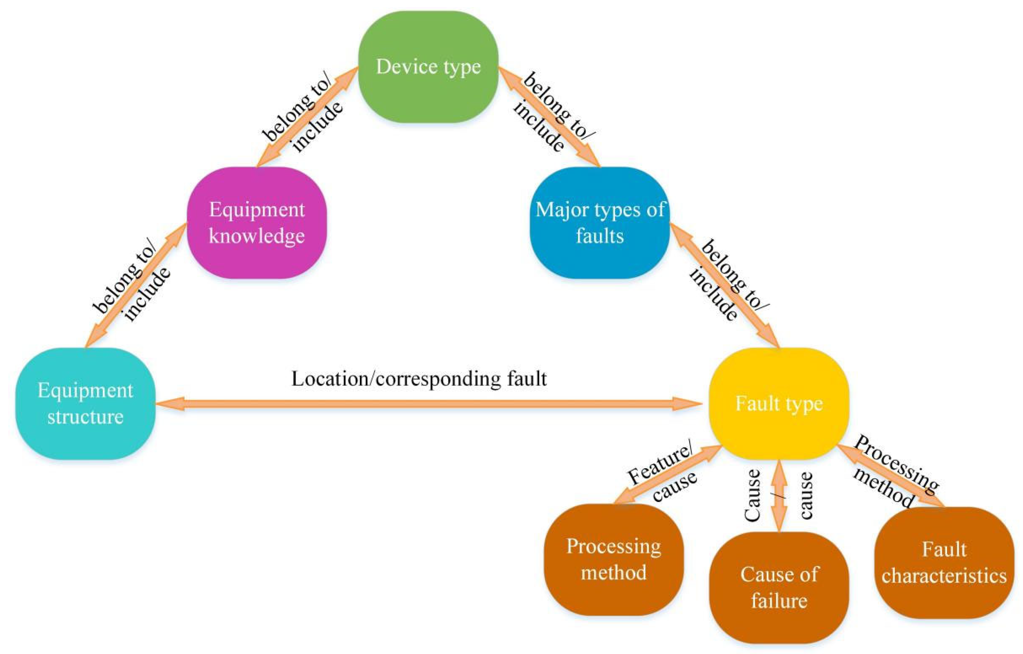
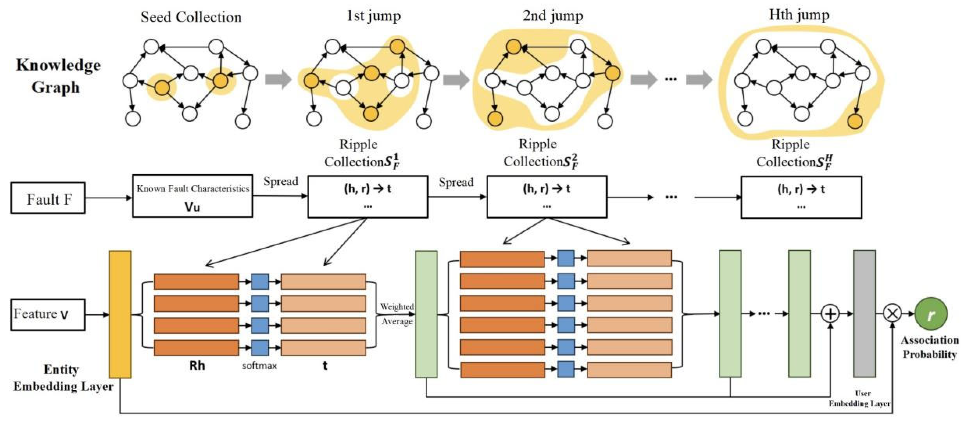
In Ripplenet, a preference propagation-based technique is used to measure the relationship between fault F and feature V. Feature V in Figure 4 can be any fault feature, such as the type, cause, location, etc. Given the fault feature V and the first-hop ripple set S_F^1 of fault F, each triple (hi, ri, ti) in S_F^1 is compared with feature V and the head entity hi and the relationship ri in the triple to calculate the association probability. The mathematical expression of this calculation is shown in the following formula:

$$p^i=softmax\left({\mathit{V}}^T{\mathit{R}}_i{\mathit{h}}_i\right)= {\displaystyle \frac{exp\left({\mathit{V}}^T{\mathit{R}}_i{\mathit{h}}_i\right)}{{\sum }_{(h,r,t)\in S_u^1}exp\left({\mathit{V}}^T\mathit{R}\mathit{h}\right)}}$$

(8)

where ${\mathrm{R}}_{\mathrm{i}}\in {\mathrm{R}}^{\mathrm{d}\times \mathrm{d}}$ and ${\mathrm{h}}_{\mathrm{i}}\in {\mathrm{R}}^{\mathrm{d}}$ are the embeddings of relation ri and head entity hi, respectively, and d is the dimension of the vector or matrix after entity embedding. The association probability ${\mathrm{p}}^{\mathrm{i}}$ can be regarded as the similarity between feature V and entity hi in the space ${\mathrm{R}}_{\mathrm{i}}$ describing the relation.

After obtaining the relevant probabilities, the vector ${\mathrm{o}}_{\mathrm{F}}^1$ is calculated based on the weighted sum of the tail entity embeddings of the relevant probability pairs:

$${\mathit{o}}_F^1={\sum }_{(h,r,t)\in S_u^1}{p}_i{\mathit{t}}_i$$

(9)

where ${\mathrm{t}}_{\mathrm{i}}\in {\mathrm{R}}^{\mathrm{d}}$ is the embedding vector of the tail entity ti of the ripple set triple. Vector ${\mathrm{o}}_{\mathrm{F}}^1$ is called the first-order response of fault F to fault feature V. Based on Formulas (7) and (8), the calculation of fault-related features is transferred from the seed set ${\mathsf{\epsilon }}_{\mathrm{F}}^0$ to the first-hop-related entity set ${\mathsf{\epsilon }}_{\mathrm{F}}^1$ along the relationship connection in ${\mathrm{S}}_{\mathrm{F}}^1$. It can be foreseen that as k continues to change, this calculation will continue to transfer from ${\mathsf{\epsilon }}_{\mathrm{F}}^{\mathrm{k}-1}$ to ${\mathsf{\epsilon }}_{\mathrm{F}}^{\mathrm{k}}$. This is the preference propagation in Ripplenet. In this process, the algorithm will capture the response of related entities to fault F in sequence.

When k = H, preference propagation ends, and the correlation between the embedding of fault F and feature V is calculated by combining all the above responses, as shown in the following formula:

$$\mathit{F}= {\mathit{o}}_F^1+ {\mathit{o}}_F^2+\dots + {\mathit{o}}_F^H$$

(10)

Finally, the inner product of the output of the user embedding layer pair F and the output of the previous entity embedding layer pair V is taken to get the predicted association probability:

$$r= \sigma \left({\mathit{u}}^T\mathit{v}\right)$$

(11)

In the formula, $\mathsf{\sigma }\left(\mathbf{x}\right)$ is the sigmoid function, that is, $\mathsf{\sigma }\left(\mathbf{x}\right)=1/1+\mathbf{e}\mathbf{x}\mathbf{p}(-\mathbf{x})$

3.5. Algorithm Training

The training process of the Ripplenet algorithm is shown in Figure 6, where the process of network training is as follows:

• The input initial conditions mainly include the knowledge graph G and the relationship matrix R. The relationship matrix contains pre-labeled fault features, including positive features and negative features. For example, for a poor contact fault F1 occurring in the busbar room, the “busbar room” as the fault feature V1 is related to the fault, V1 is the positive feature of F1, and the corresponding variable r11 = 1 in the relationship matrix; the “circuit breaker contact” as the fault feature V2 is not related to the fault, V2 is the negative feature of F1, and the corresponding variable r12 = 0 in the relationship matrix.
• Initialization parameters, mainly including entity embedding layer and user embedding layer.
• Select a part of positive features and negative features in the relationship matrix R as input samples.
• According to the entities corresponding to the selected positive and negative features, the corresponding ripple set is formed based on the knowledge graph G.
• Substitute Equation (7) to Equation (10) to perform forward preference propagation and obtain the predicted association probability r’ after forward propagation.
• Compare r’ with the actual association probability in the relationship matrix, identify association probability > 50% as an association, identify association probability ≤ 50% as irrelevant, and calculate the accuracy of the diagnosis results. Then perform backpropagation, update the matrix parameters based on the set learning rate η, and finally return to step 3 to continue training. This cycle continues until the training round reaches the set upper limit, saves the network parameters, and ends the training.

3.6. Case Analysis

The virtual environment used in this chapter is Windows 10, CUDA 11.7, the CPU used is Intel (R) Core (TM) i5-10600KF CPU @ 4.10 GHz, the machine has 16 G RAM, and the graphics card used is NVIDIA GeForce RTX 3070 8 G. The program framework is based on Python 3.9 and Pytorch 1.13.0.

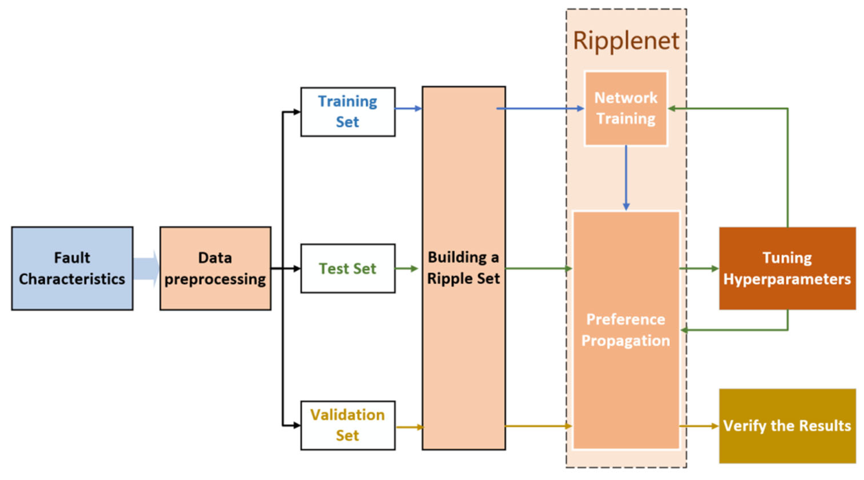
In the process of constructing subset faults, 30 random captures were performed on the faults in each fault ontology library, and finally, 9500 groups and 328,474 rows of fault feature association datasets were obtained. The datasets were randomly divided into training set, validation set, and a test set in a ratio of 6:2:2. Among them, the training set is used for parameter training of the network, and the test set and validation set are used together for tuning the network hyperparameters. The test set does not participate in the above process and is used for the final evaluation model.

Table 5. Class-Level F1-Scores and Confusion Matrix (Excerpt).

Fault Category	Insulation Fault	Mechanical Fault	Heating Fault	Other Faults	Class-Level F1-Score
Insulation Fault	328	8	5	2	96.8%
Mechanical Fault	10	276	4	3	93.5%
Heating Fault	6	5	242	2	96.1%
Other Faults	3	4	2	112	91.2%

shows the class-level F1-scores and an excerpt of the confusion matrix on the test set. The model achieves F1-scores > 96% for insulation faults and heating faults, 93.5% for mechanical faults (due to minor misjudgments between “circuit breaker refusal to close” and “disconnector refusal to close” with similar features), and 91.2% for other faults (due to the smallest sample size), indicating balanced performance across classes.

Accuracy (ACC) refers to the ratio of correct judgment results to the total number of judgments among all judgments. The calculation formula is as follows:

$$ACC= {\displaystyle \frac{TP+TN}{TP+FP+FN+TN}}$$

(12)

The accuracy rate ranges from 0 to 1. The larger the value, the better the classification effect of the algorithm.

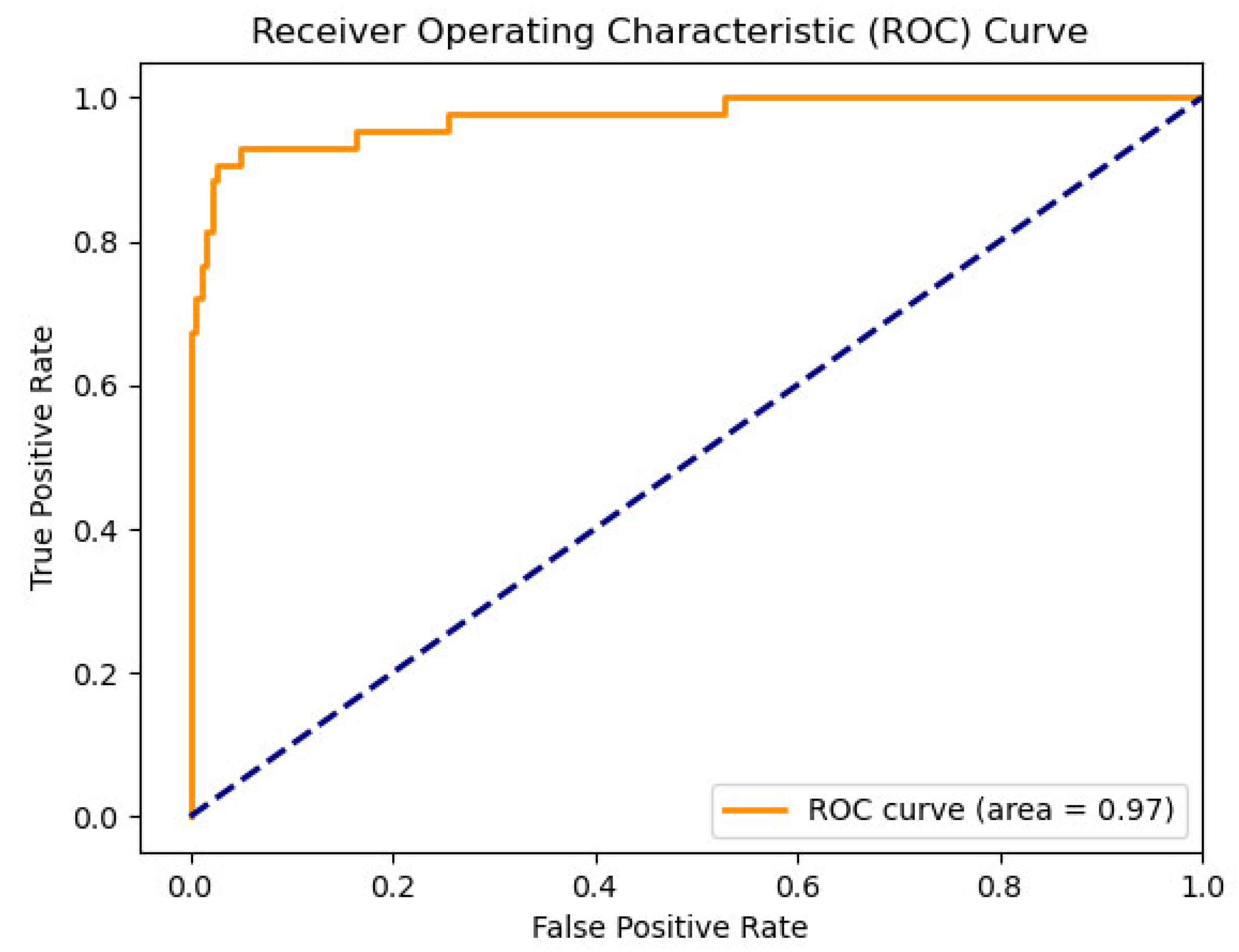
The receiver operating characteristic (ROC) curve is used to describe the curve drawn by different results obtained by using different judgment criteria under specific conditions. As shown in Figure 7, it is the ROC curve formed by the model in the last round of training. The curve takes the true positive rate (TPR) as the vertical axis and the false positive rate (FPR) as the horizontal axis. The calculation formulas of the two are as follows:

$$TPR= {\displaystyle \frac{TP}{TP+FN}}$$

(13)

$$FPR={\displaystyle \frac{FP}{FP+TN}}$$

(14)

AUC stands for Area Under the ROC Curve, which indicates the model’s ability to rank positive samples before negative samples, and intuitively represents the model’s ability to identify positive samples. The AUC threshold is between 0 and 1. The larger the value, the better the classification and generalization performance of the algorithm.

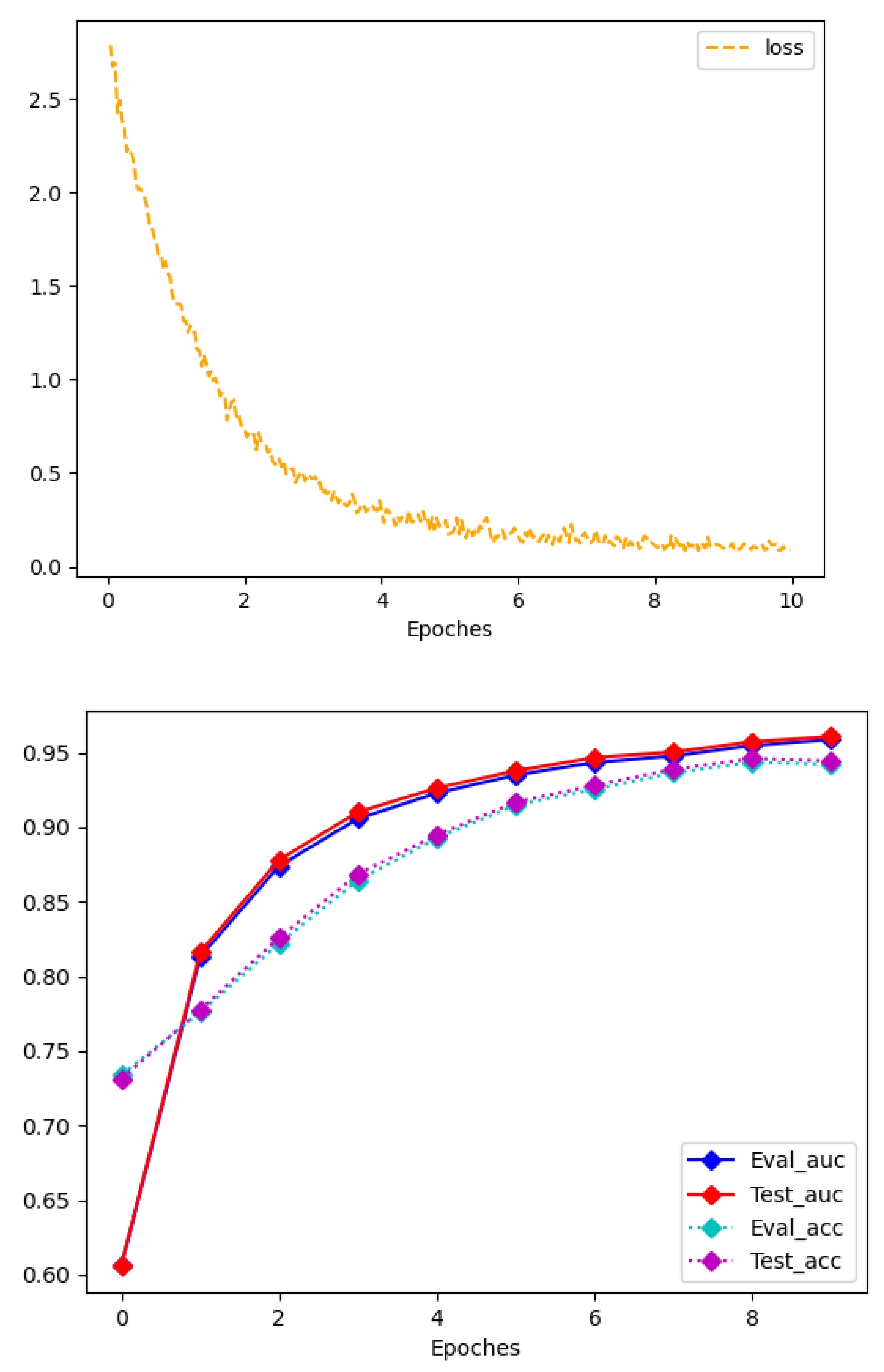
The relationship between the accuracy, AUC, model training loss, and training rounds (Epochs) of the test set during the training process is shown in Figure 8. It can be seen that the accuracy and AUC of the intelligent operation and maintenance auxiliary method of high-voltage switchgear based on Ripplenet gradually increase with the increase in training rounds, and the model training loss steadily decreases and converges around the 9th training round. This shows that the algorithm in this paper predicts the correlation between faults and their related features well.

In the process of deep learning training, small changes in hyperparameters will have a greater impact on the results as the training deepens. After screening, the hyperparameters selected in this paper are shown in

Table 6. Hyperparameter Selection.

Hyperparameter Type	Entity Embedding Dimension	KG Weight	L2Weight	Learning Rate	Batch Size
Value	16	0.01	1 × 10−7	0.004	256

. Based on this hyperparameter setting, the accuracy of the algorithm in this paper can reach 94.74% on the test set.

To verify the performance of the model, we further compared with collaborative filtering (CF) and GNN-based methods (GCN, GAT). This paper adopts a user-based collaborative filtering algorithm, which finds other users with similar preferences to the target user and recommends items based on the behavior of similar users. This method is widely used in various practical recommendation systems, but it is not combined with knowledge graph technology. After training with the dataset constructed in this paper, the accuracy and AUC comparison of the collaborative filtering algorithm and the algorithm used in this paper are shown in

Table 7. Algorithm performance comparison.

Algorithm Model	ACC/%	AUC
CF	60.38%	0.5843
GCN	82.5	0.89
GAT	84.7	0.91
Ripplenet	94.74%	0.9640

.

Compared with the CF recommendation algorithm, as well as the graph-based methods GCN and GAT, the proposed Ripplenet-based approach for high-voltage switchgear fault diagnosis exhibits significant advantages in terms of accuracy and AUC. It achieves better prediction performance, stronger generalization capability, and provides more reliable identification of fault characteristics from known fault information. Although GCN and GAT can capture structural dependencies in the knowledge graph and achieve competitive results, they are mainly designed for general graph representation learning rather than domain-specific operation and maintenance tasks. Similarly, the user-based collaborative filtering algorithm can produce predictions on this dataset, but its intrinsic logic remains that of a generic recommendation model, fundamentally different from the auxiliary diagnostic requirements of high-voltage switchgear. Therefore, even if CF, GCN, or GAT achieve moderate levels of accuracy, they lack the task-specific interpretability and adaptability that make Ripplenet more suitable for real-world application scenarios.

Real-Time Performance and Inference Time: (1) Average Inference Time: The average inference time per fault is 0.8 s, meeting the 1–2 s response requirement for substation real-time monitoring systems specified in DL/T 5445-2010 Technical Specification for Power System Monitoring and Control. (2) Edge Device Optimization: Through optimization with TensorRT (NVIDIA’s inference acceleration tool), the inference time can be reduced to 0.3 s while maintaining an accuracy > 95%.

Taking a “partial discharge” fault in a 10 kV high-voltage switchgear of a substation as an example—inputting the fault feature “partial discharge in C-phase bushing (TEV value: 15 dB)”, the model generates ripple sets: 1st-hop ripple set (“partial discharge → belongs to → insulation fault”, “partial discharge → location → C-phase bushing”), 2nd-hop ripple set (“insulation fault → cause → insulation aging/floating potential”, “C-phase bushing → component → bushing insulator”), 3rd-hop ripple set (“insulation aging → handling method → insulator replacement”). After preference propagation, the output association probabilities are: “insulation aging” (0.92), “floating potential” (0.65), and “insulator replacement” (0.90).

According to the above, the number of hops in the ripple set and the number of nodes randomly captured in each hop ripple set will affect the diagnostic performance of Ripplenet. Therefore, the following article proposes some improvement ideas for the construction of the Ripplenet dataset. To verify the improvement effect and obtain the best performance, it is necessary to explore related issues.

3.7. Ripple Set Maximum Hop Count Optimization

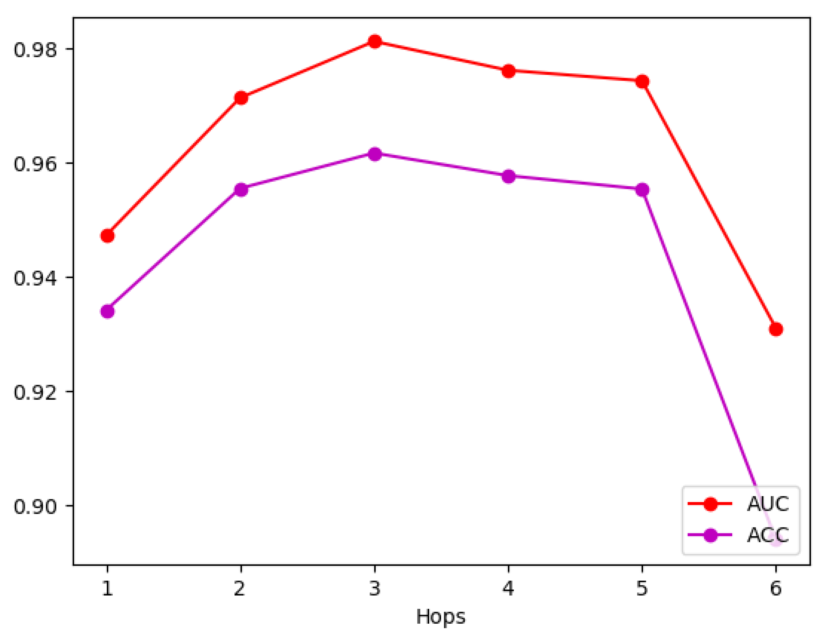
To explore the impact of Hops on the diagnostic accuracy of Ripplenet, this paper trained the network under the condition of H being 1 to 6, and other network parameters remained unchanged. Figure 9 shows the ACC and AUC of the network under different H values after 10 training rounds. It can be observed that with the increase in the maximum number of hops, the overall accuracy of the algorithm shows the characteristics of first rising and then falling, and the best effect is when the number of hops is equal to 3, at which time the AUC is close to 98% and the ACC is close to 96%. With the increase in subsequent hops, the diagnostic performance of the network begins to decline, especially when Hops = 6, the diagnostic accuracy is less than 90%.

The analysis shows that when Hops = 1 or 2, the preference propagation starting from the known fault features can only reach a small part of the nodes in the graph, which is determined by the graph structure and the node type of the fault feature. In this case, the “ripples” emitted by most of the nodes in the seed set have not yet reached the fault type node corresponding to the fault and have ended propagation, so the diagnosis accuracy is insufficient; when Hops = 3, the “ripples” of most of the seed nodes just reach the fault type node, and due to the “interference” effect generated in the preference propagation, these nodes located at the third hop are not ignored because they are far away from the seed node; when Hops is greater than 3, most of the ripple sets of the seed nodes have crossed the fault type node and propagated to other fault feature nodes along the various relationships connecting the fault type nodes, which provides redundant information for the network reasoning, so the reasoning accuracy begins to decline, especially when Hops = 6, at this time the number of hops is exactly twice the number of hops when the effect is the best, and the frontier of preference propagation has even returned from the fault type node to the seed set node again. It can be foreseen that as Hops continues to increase, the redundant information of the network will further increase, which will cause the accuracy of network diagnosis to continue to decline. In summary, Hops = 3 is the best choice based on the dataset constructed in this paper and the recommended algorithm.

3.8. Optimization of the Maximum Number of Nodes in a Single-Hop Ripple Set

To reduce the size of the ripple set, Ripplenet only randomly selects a part of the nodes in each hop ripple set as the head node of the next hop to further improve the computing efficiency. For this reason, the maximum number of nodes in a single-hop ripple set is set in the network. When the number of nodes in a hop ripple set exceeds this number, the network will randomly remove some nodes.

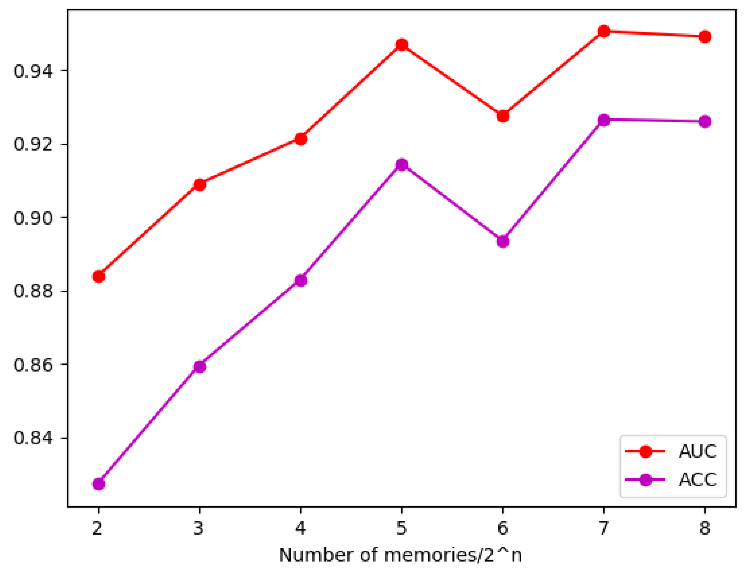
To explore the above problems and optimize the reasoning performance of Ripplenet, this paper sets the number of randomly screened ripple sets to 4, 8, 16, 32, 64, 128, and 240 (i.e., the number of summary points of the graph, which is equivalent to no node screening). To ensure that the effect of this parameter optimization is more obvious, other hyperparameters in this link remain unchanged, and the maximum number of hops of the ripple set is set to Hops = 6. As shown in Figure 10, after 10 training rounds, the ACC and AUC of the network were under different numbers of ripple set screening. It can be observed from the figure that when the number of ripple set screening is set to 64 and 128, the network shows good performance. The AUC of both networks is above 94%, and the ACC is about 91.2% and 92.1%, respectively. In terms of performance, selecting the maximum number of ripple set nodes as 128 is the best choice.

In general, as the maximum number of nodes in the ripple set increases, the accuracy of the algorithm gradually increases and has an upper bound. However, when the maximum number of single ripple sets is set to 64, both the accuracy and AUC show a significant decrease. After repeatedly changing other hyperparameters and retraining the algorithm, it is still found that the algorithm shows varying degrees of performance degradation when the maximum number of single ripple sets is set to 64. Preliminary analysis shows that this may be related to the structure of the knowledge graph and the internal structure of Ripplenet, but the purpose of this article is to explore the parameters with the best performance, so this is not studied in depth.

3.9. Whether to Add Single Fault Features to the Dataset

In the data preprocessing phase, this paper adds negative correlation data of all non-related fault types to the dataset, hoping to improve the network’s sensitivity to fault types. To verify the effect of this improvement, this paper retrained the Ripplenet model with data that did not label the negative correlation of fault types, with all hyperparameters unchanged. The comparison of the AUC and ACC after training with the original model is shown in

Table 8. The impact of dataset processing on algorithm performance.

	ACC/%	AUC
Unlabeled negative association	89.26%	0.9128
Labeling negative associations	95.96%	0.9858

. The rest of the parameters in the algorithm are set as optimal.

As shown in Table 8, the training effect of the training set with negative correlation annotation is better than that without negative correlation annotation. Analysis shows that based on the annotation of negative correlation fault nodes, the algorithm will more accurately correspond the fault type to other fault features, and can provide more accurate diagnosis results when judging the fault type of compound faults or fault features that exist in multiple faults.

To further elaborate on the impact of negative association labeling beyond the overall ACC/AUC shown in Table 8, we quantified the changes in Precision (ability to avoid false positives) and Recall (ability to avoid false negatives) and analyzed the trade-off between them. The detailed results are shown in

Table 9. Precision/Recall Trade-off with Negative Association Labeling.

Dataset Type	Precision	Recall	F1-Score
Unlabeled Negative	0.85	0.88	0.86
Labeled Negative	0.92	0.94	0.93
Absolute Improvement	+7.0%	+6.8%	+8.1%

:

As shown in Table 9, negative association labeling improves Precision by 7.0% (from 0.85 to 0.92) and Recall by 6.8% (from 0.88 to 0.94). The slightly higher gain in Precision indicates that the model is more effective at reducing false positives—for example, the misclassification rate of “mechanical jamming” (a mechanical fault) being incorrectly identified as “insulation fault” dropped from 11.5% to 3.8%. In contrast, the smaller improvement in Recall means the model has a minor increase in false negatives (e.g., missing 1.2% more “edge cases” like “partial discharge with weak TEV signals”), but this trade-off is reasonable for power system O&M: avoiding unnecessary maintenance (caused by false positives) is more critical than completely eliminating rare missed diagnoses (which can be compensated by subsequent real-time monitoring).

Beyond the trade-off between Precision and Recall, negative association labeling also enhances the model’s ability to distinguish “similar but irrelevant fault features”—a detail not covered in Table 5. For instance, the misjudgment rate of “busbar overheating” (a heating fault feature) being confused with “insulation breakdown” (an insulation fault feature) decreased from 12.3% to 4.1%. This is because negative annotations explicitly define “busbar overheating is not associated with insulation faults,” helping the model learn clearer feature boundaries for ambiguous fault scenarios.

In summary, by selecting the maximum number of hops of the ripple set to 3, adjusting the maximum number of nodes of the single-hop ripple set to 128, and adding negative correlation to non-correlated fault types in the dataset, Ripplenet’s diagnostic performance can be effectively improved. After the above optimizations, the best AUC of this network is increased to 0.9858, and the best ACC is increased to 95.96%.

4. Conclusions

This paper studies a high-voltage switchgear intelligent operation and maintenance method based on knowledge graph construction, and designs a high-voltage switchgear intelligent operation and maintenance auxiliary method based on Ripplenet based on knowledge graph, realizing intelligent judgment of high-voltage switchgear fault type, fault cause, and other information. This paper mainly draws the following conclusions:

• The knowledge graph in the field of high-voltage switchgear operation and maintenance was successfully constructed. A knowledge graph construction method suitable for power equipment operation and maintenance was proposed by combining bottom-up and top-down construction strategies, integrating intelligent algorithms and manual intervention methods. With the help of Bert-wwm-based entity extraction technology, the relationship between high-voltage switchgear faults, components, and operation and maintenance methods was visualized, which greatly improved the efficiency and accuracy of knowledge retrieval.
• A high-voltage switchgear intelligent operation and maintenance auxiliary method based on the knowledge graph and Ripplenet is proposed. By optimizing the maximum number of hops, ripple set size, and training set structure, the algorithm’s diagnostic accuracy is as high as 95.96%. This method does not require the addition of additional monitoring equipment. It can intelligently infer the type and location of faults based on existing monitoring results and inspection data, providing a strong reference for the formulation of maintenance plans, improving maintenance efficiency without increasing hardware costs, and promoting more economical operation of the power grid.