Abstract
Designing an effective electrical model for charged water bodies is of great significance in reducing the risk of electric shock in water and enhancing the safety and reliability of electrical equipment. Aiming to resolve the problems faced in using existing charged water body modeling methods, a practical circuit model of a charged water body is developed. The basic units of the model are simply constructed using fractional-order resistance–capacitance (RC) parallel circuits. The state variables of the model can be obtained by solving the circuit equations. In addition, a practical method for obtaining the circuit model parameters is also developed. This enables the estimation of the characteristics of charged water bodies under different conditions through model simulation. The effectiveness of the proposed method is verified by comparing the estimated voltage and leakage current of the model with the actual measured values. The comparison results show that the estimated value of the model is close to the actual characteristics of the charged water body.
1. Introduction
With the widespread application of electrical equipment, electric shock accidents triggered by leakage current have become a common occurrence [1]. When electrical devices suffer from current leakage, the leakage current is likely to flow toward the ground. Under severe weather conditions such as heavy rainfall and typhoons, the ground is highly susceptible to water accumulation. Once the leakage current enters the accumulated water, its propagation path and intensity may be enhanced—this significantly elevates the risk of electric shock accidents [2]. Consequently, there is an urgent demand for the development of an effective early warning method, which can assist in the prevention of electric shock incidents.
When water comes into contact with charged objects, an electric field is generated and current distribution takes place. The electric field and current are determined by the voltage of the external charged object, as well as the spatial distribution and conductivity of the water [3]. A precise equivalent circuit model can act as the key theoretical basis for active electric shock early-warning and protection systems, and risk reduction can be achieved by incorporating a model such as a core component into these systems. In the event of an electrical leakage fault, current may be injected into a water body, causing it to become energized. A precise equivalent model enables the calculation and prediction of the potential gradient at various points within the water. Based on the aforementioned calculations and with reference to international safety standards for human body current/voltage thresholds, it becomes feasible to quantify hazardous and safe zones—specifically, to derive a critical safety distance for electric shock prevention. For example, the system could define a specific radius from the leakage point as a danger zone. Furthermore, by leveraging this model, an intelligent early-warning system can be developed; equipped with sensors, this system could monitor the electrical parameters of the water in real time or at regular intervals. Therefore, establishing an effective electrical characteristic model for water is of great significance for reducing the risk of electric shock in water and improving the safety and reliability of electrical equipment.
Several methods have been developed for establishing charged water body models, among which the finite element method (FEM) and the boundary element method (BEM) are typical approaches [4]. The FEM addresses more complex geometries by subdividing the water body into small elements and solving differential equations based on the physical properties of the water. However, in some cases, this method may require significant computational resources and time [5]. The BEM transforms the problem into integral equations on the boundary, thereby improving computational efficiency; yet, it may still face challenges when dealing with scenarios involving complex material behaviors. Therefore, developing a simple and effective model for charged water bodies remains an open issue that requires further study.
To address the limitations of the aforementioned existing methods, a charged water body model based on the resistance-capacitance (RC) network is developed in this paper. This model simulates the electrical characteristics of charged water bodies through the combination of circuit elements, enabling the derivation of state variables such as voltage and current by solving circuit equations. This approach avoids the need to solve complex mathematical and physical equations, thereby effectively simplifying the simulation process.
In recent years, research has been conducted on the fractional-order characteristics of actual systems [6,7]. Traditional integer-order models are built on the assumption of ideal, memoryless diffusion. However, studies have shown that ion migration in real moist environments—constrained by surface charge heterogeneity and complex ion–molecule interactions—exhibits the characteristics of anomalous diffusion [8]. Additionally, the existing literature indicates that traditional models exhibit significant deviations between theoretical results and experimental data in the low-frequency region [9]. The convolution integral kernel of fractional differential operators naturally provides a mathematical description of this “non-local” spatiotemporal correlation. By introducing an additional degree of freedom, the frequency response of the fractional-order model can accurately fit experimental data over a broader frequency band, particularly in the low-frequency region.
Moreover, capacitors have been reported to exhibit fractional-order memory characteristics, attributed to the nano-architected material and structure of their electrodes, as well as their electrochemical design [10]. The spectral impedance of such capacitors shows a distinct deviation from the −90° phase angle of an ideal capacitor [11]. The fractional-order capacitor serves as a standard modeling tool for non-ideal capacitive behavior. The frequency-domain impedance of this model yields a constant phase angle of . When , the absolute value of the phase angle is less than 90°, which directly corresponds to the non-ideal state and active power loss of practical capacitors [12,13]. Building on existing findings, this paper incorporates the fractional-order characteristics of capacitors. Specifically, a fractional-order capacitor is introduced to form the basic RC parallel circuit unit of the water model. The effectiveness of the proposed model is verified by comparing the estimated results with those obtained from actual experiments.
The main contributions of this paper include the following: (1) A fractional-order resistance-capacitance (RC) circuit-based network model for charged water bodies is designed, which provides an accurate description of the electrical characteristics of charged water bodies. (2) A method for solving various physical quantities within the charged water body model is developed, offering a simple and practical approach for simulating charged water body scenarios. (3) A practical method for acquiring the network parameters is designed, thus forming a complete model construction and simulation scheme for charged water bodies.
The rest of this paper is arranged as follows: preliminary knowledge about the fractional calculus is presented in Section 2; the fractional-order RC circuit-based model is developed in Section 3; the model parameter acquisition method is presented in Section 4; the efficiency of the proposed model is verified in Section 5; and the conclusion is discussed in Section 6.
2. Preliminary Knowledge
2.1. Fractional Calculus
Fractional calculus extends the orders of the differentiation and integration to arbitrary orders, which can be real numbers or even complex numbers. The fundamental operator of fractional calculus is expressed as , where a and t represent the upper and lower limits of the operator, respectively, and is the fractional order of differentiation/integration. The -th derivative of a function is given as
It can be seen that the fractional differential operator unifies fractional differentiation and integration. When Re() > 0, denotes fractional differentiation, and when Re() < 0, it represents fractional integration. When is a positive integer n, signifies the n-th derivative of the function . Therefore, integer-order calculus is a special case of fractional calculus.
2.2. Definition of Caputo Fractional Calculus
The Caputo fractional differentiation [14] is defined as
where m is the largest natural number smaller than , , is the gamma function. The definition of the Caputo fractional integration [14] is given by
The unified definition of Caputo fractional calculus is presented as
3. RC Network-Based Model
3.1. Basic Unit
The circuit network model of the charged water body is made up of M, N and L layers of basic units in the spatial three-dimensional coordinates x, y and z. The basic unit of the network is a tetrahedron, as shown in Figure 1. Each unit is labeled as (), where i, j and k represent the indexes of the unit in the network in x, y and z axes, respectively. The positive direction of the x, y and z coordinate axes lies in which the labels i, j and k increase. The unit has three impedance branches, and the state variables include the node voltage and the currents flowing into the three impedance branches, and . The state vector of each unit can be represented as .
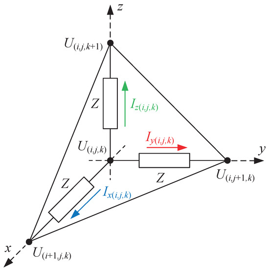
Figure 1.
Basic tetrahedral unit model.
3.2. Node Mathematical Model
The aqueous model is developed according to the specific physical context and application scenario of this study, which focuses on electrical leakage warning and protection for equipment near water bodies. The water acts as a dielectric medium, forming a capacitive structure with other surrounding conductors. This leads to interfacial charge separation and energy storage phenomena; while inductive effects are universally present, their magnitude is highly dependent on the application’s spatial scale, frequency and conductivity. The primary signals of interest for leakage warning are power frequency (50/60 Hz) and their low-order harmonics. At these frequencies, and given the relatively high conductivity of ionic water, the resistive and capacitive impedances dominate the system’s response. Therefore, a distributed RC network is adopted in this paper, and a parallel combination of a resistor R and a fractional-order capacitor are adopted to form the impedance branch of the basic unit [15], as shown in Figure 2. Based on the grid unit model shown in Figure 1 and the impedance branch model shown in Figure 2, the current equations through the impedance branches in the x, y and z directions can be derived as follows [16,17]:
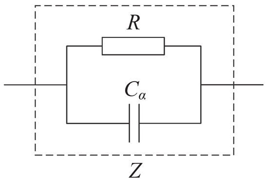
Figure 2.
Fractional order RC model of the impedance branch.
In addition, the sum of the currents in the impedance branches in the three directions satisfies (8) [18,19],
where , and represent the impedance branch currents of the adjacent units, and denotes the current injected into the node from external source, like electrode (for passive nodes, ). Equations (5)–(8) are the fundamental unit differential equations.
The fractional-order differentiation is implemented using a discretization method based on the impulse response invariant principle [20]. The fractional-order differential operator is approximated as a discrete transfer function by specifying the sampling time and approximation order m, as represented by (9),
where z is the complex variable. Substituting (9) into Equations (5)–(7), difference equations for the nodes can be obtained as follows:
In addition, the following difference equation can be obtained from (8):
where n denotes the index of the sampling points.
3.3. Node Classification and Boundary Conditions
Equations (10)–(13) represent the fundamental equations satisfied by each network node. In fact, when nodes are located at different positions or under different external conditions, the general equation needs to be converted to the corresponding boundary conditions. According to their positions within the network, nodes can be primarily classified as internal nodes or boundary nodes. Internal nodes are located inside the network, i.e., surrounded by other nodes. Boundary nodes are located at the edge of the network; namely, in at least one of the x, y and z directions, no other node is connected to them. Depending on their locations, boundary nodes can be further categorized into upper and lower boundary nodes. Considering the external conditions affecting the nodes, their states can be characterized as grounded, insulated, passive or active, respectively.
- A.
- Internal Nodes
In this paper, for a clear illustration of the node types, the network is displayed in two dimensions in all figures. An example of the internal node is marked in green in the network depicted in Figure 3. These nodes are located within the network and fully connected to other nodes. According to the external condition, these nodes can be categorized into three types: internal passive nodes, internal active nodes, and internal grounded nodes.
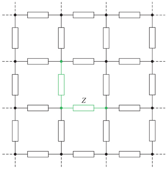
Figure 3.
Internal node.
- (1)
- Internal passive node:
Internal passive nodes are not subject to specific boundary conditions and instead adhere to the general Equations (10)–(13).
- (2)
- Internal active node:
The voltage of an internal active node is equal to the external source voltage , but the external injected current is unknown. Therefore, (13) is modified to the boundary condition , that is
- (3)
- Internal grounded node:
An internal grounded node is equivalent to an active node with external voltage of 0. Therefore, (13) is modified to the boundary condition,
- B.
- Upper Boundary Nodes
Upper boundary nodes are located at the uppermost layer of the network, where the grid indices or k attain their maximum values. Two examples of the upper boundary nodes are marked in red and blue in Figure 4. These nodes have two distinct states: grounded or insulated.
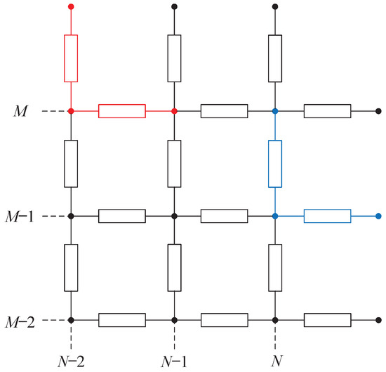
Figure 4.
Upper boundary node.
- (1)
- Upper boundary grounded node:
First, (13) is modified to boundary condition (15) based on the condition that the voltage of the grounded node is set to zero. Second, the voltage at the boundary endpoint of the node is also set to zero. For instance, if the node is located on the x-axis boundary, i.e., i = M, as marked in red in Figure 5, then the boundary condition = 0 can be obtained, and (10) is modified to the boundary condition as follows:
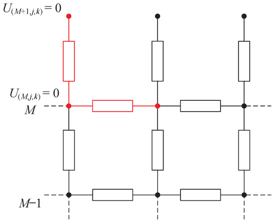
Figure 5.
Upper boundary grounded node.
Considering that = 0, boundary condition (16) is actually equivalent to = 0.
Similarly, if the node is located at the boundary along the y-axis, specifically where , the boundary condition is = 0, then (11) is modified to
Finally, if the node is located at the boundary along the z-axis, specifically where k = L, the boundary condition is = 0, and then (12) is modified to
- (2)
- Upper boundary insulated node:
For an upper boundary node, if there is no adjacent node lying in the x, y or z direction, the current in the impedance branch in that direction is 0. If the node is located at the boundary along the x-axis, specifically where i = M, the boundary condition is = 0, as marked in red in Figure 6. Consequently, (10) is modified to
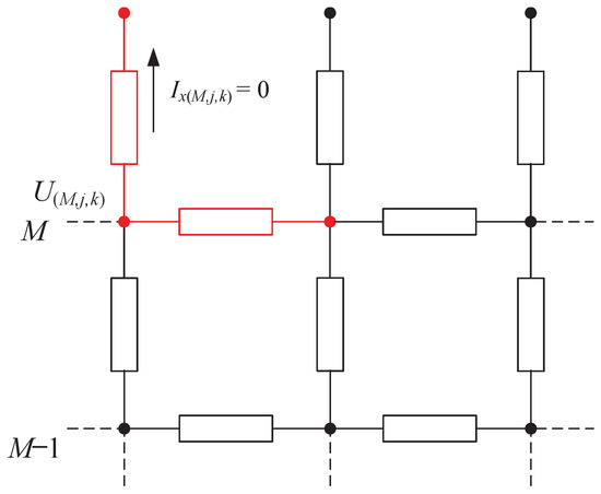
Figure 6.
Upper boundary insulated node.
Similarly, if the node is located at the boundary along the y-axis, specifically where , the boundary condition is = 0, and (11) is modified to
Finally, if the node is located at the boundary along the z-axis, specifically where , the boundary condition is = 0, and (12) is modified to
- C.
- Lower Boundary Nodes
Lower boundary nodes are situated at the lowermost layer of the water body model, where the grid indices i, j or k are at their minimum values. These nodes, like their upper boundary counterparts, have two states: grounded or insulated.
- (1)
- Lower boundary grounded node:
When a lower boundary node is grounded, its voltage is set to 0. Consequently, the boundary condition for this node mirrors that of an internal grounded node. Thus, (13) is modified to boundary condition (15).
- (2)
- Lower boundary insulated node:
Nodes situated at the lower boundary do not have input current from the impedance branch of the lower unit. For instance, if a node is marked as the lower boundary of an x-axis unit (i = 1), the currents entering the node include and , as shown in Figure 7. If the node is insulated without any external injected current, and the boundary condition includes = 0, then the term in (13) should be set to 0.
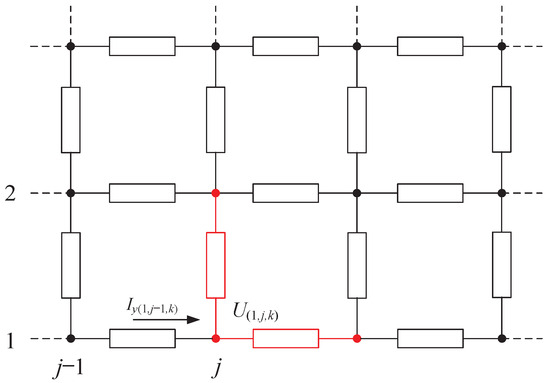
Figure 7.
Lower boundary insulated node.
If the node is the lower boundary of a y-axis unit (), and the boundary condition includes = 0, the term in (13) should be 0. Similarly, if the node is the lower boundary of a z-axis unit (k = 1), the boundary condition includes = 0, and the term in (13) should be 0.
- D.
- Solution for for node state variables
Each node’s state vector in the network has four state variables to be solved. The state variables are governed by four equations (basic and boundary conditions). However, these equations contain the states of the adjacent nodes. To obtain the states of each node, the equations of all nodes should be solved.
Combining the equations of all nodes, the linear equations of the whole impedance network can be obtained X = Y. The vector X is constructed by connecting the state vectors of all nodes, , containing a total of elements. is a matrix, containing the coefficients of the linear equations. For example, assuming the node () is an internal active node satisfying (10) to (13), the corresponding element in matrix is
where
The remaining elements in rows of matrix are zero. Since the state of each node is only associated with the states of its adjacent nodes, matrix is a sparse matrix.
Y is a vector composed of terms other than the node states in the equations of each node, including the node voltage, branch current, and external power supply voltage in the past sampling time points. For example, the elements of vector Y corresponding to the internal active node () are
By solving the linear equation , a unique solution for the states of each node can be obtained.
Active nodes and grounded nodes may have external injected currents . After calculating the state variables of each node, the external injected currents for each node can be calculated as follows,
4. Model Parameter Acquisition
The impedance branch model for each unit within the network model is depicted in Figure 2. The parameters to be determined are the resistance R, capacitance C, and fractional order [21].
4.1. Network Setup
The computation for solving the physical quantities of the impedance network increases with the grid density. The more grids within the same distance, the greater the computational load. To avoid excessive computation in some cases, a scalable grid is adopted; namely, when the actual distance between electrodes changes, the grid size adjusts accordingly, while the number of grids between the electrodes is maintained at a fixed value. This value can be set within a given range based on actual needs: if a rough distribution of voltage and current is required, fewer grid points (larger grid size) can be selected; if more detailed results are needed, more grid points (smaller grid size) can be chosen.
To ensure the effectiveness of the scalable grid, when selecting different grid sizes under the same electrode spacing, the equivalent resistance and capacitance of the water between the electrodes should be equal or close to equal. First, the relationship between the grid unit resistance and the equivalent resistance between electrodes is studied. The simplest way is to set a fixed resistance value for the grid units of different sizes. According to this assumption, the relationship between the number of grids between electrodes and the equivalent resistance value between electrodes is obtained, as depicted in Figure 8.
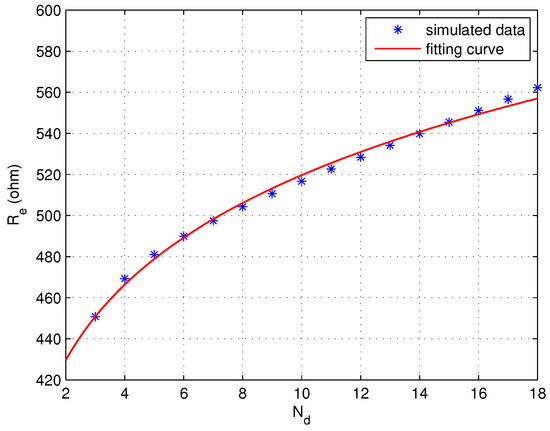
Figure 8.
Variation of with under fixed electrode spacing.
As shown in Figure 8, if a fixed grid unit resistance is used, the equivalent resistance between electrodes increases with the number of grids between the electrodes, and presents a nonlinear growth relationship, which is obviously not in line with the requirements. To achieve a constant , it is necessary to adjust the unit resistance according to the grid number [22].
According to the feature of the relationship between and shown in Figure 8, the power function is used to describe the law of changing with . Furthermore, since depends on the grid unit resistance R, it is reasonable to infer that the larger the resistance R of the grid unit, the larger the equivalent resistance . Therefore, a linear relationship between R and is assumed. Based on these two assumptions, the expression of is formulated as
where R denotes the grid unit resistance, and is a constant to be determined.
In order to keep constant under different number of grids, the grid unit resistance needs to be adjusted based on . Therefore, the expression for R is assumed to be
where is a constant, and is a function related to the distance between electrodes. In this way, the term in (33) can be cancelled by the corresponding term in (34), ensuring that remains constant for different values of . Fitting the data points of changing with , the parameter = 0.115 is obtained.
The adjusted grid unit resistance is adopted in the network for simulation, and the relationship between and is obtained, as shown in Figure 9. It can be seen that, after adjusting the grid unit resistance, when ranges from 3 to 15, the equivalent resistance remains within a relatively fixed range. Therefore, the range of is specified between 3 and 15.
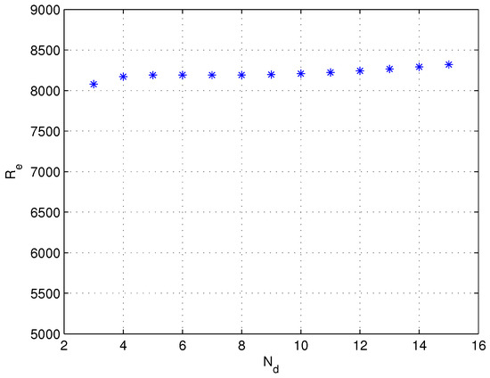
Figure 9.
Variation in with under fixed electrode spacing when the adjusted unit resistance is used.
The same method is used to study the relationship between the grid unit capacitance and the equivalent capacitance between electrodes. If a fixed capacitance value is set for grid units with different sizes, the relationship between the number of grids and the equivalent capacitance between electrodes is obtained and shown in Figure 10.
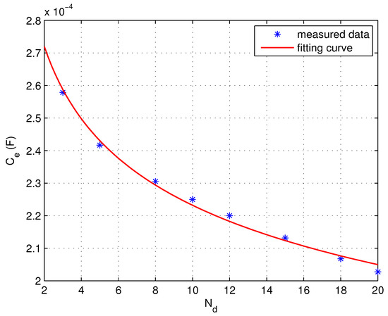
Figure 10.
Variation in with under fixed electrode spacing.
It can be seen that, if a fixed grid unit capacitance is used, the equivalent capacitance between electrodes decreases with the increase in the number of between electrodes, and presents a nonlinear relationship, which does not meet the requirements. To sustain a constant equivalent capacitance, the grid unit capacitance needs to be adjusted.
According to the relationship between and shown in Figure 10, the power function is used to describe the law of changing with . Furthermore, since the equivalent capacitance is correlated with the grid unit capacitance C, it is reasonable to deduce that the larger the grid unit capacitance C, the larger the equivalent capacitance . Therefore, a linear relationship between C and is assumed, and then the expression of is formulated as
where is a constant to be determined.
Under different numbers of grids, to keep the equivalent capacitance constant, the capacitance of the grid units C needs to be adjusted based on . Therefore, the expression for C is assumed to be
where is a constant, and represents a function of the distance between electrodes. Consequently, the term in (35) is cancelled by the corresponding term in (36), ensuring that remains unchanged when takes different values.
The parameter is determined by fitting the data points of varying with , obtaining = 0.123. The fitting curve is illustrated in Figure 10.
The adjusted grid unit capacitance is adopted in the network simulation, and the relationship between the equivalent capacitance and is presented in Figure 11. It can be seen that, following the adjustment of the grid unit capacitance, remains within a relatively stable range when varies between 3 and 15. Hence, the range for is set as 3 to 15.
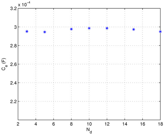
Figure 11.
Variation in with under fixed electrode spacing when the adjusted unit capacitance is used.
4.2. Acquisition of Resistance R
To determine , the relationship between electrode spacing (D) and equivalent resistance () is investigated. A measurement experiment is performed: a pair of electrodes are immersed in water and connected to a DC power supply. Then a loop connecting the power source and the water is formed. The input voltage is increased gradually while both the input voltage and loop current are recorded simultaneously. For a fixed electrode spacing, the voltage-current () characteristic curve is obtained, as shown in Figure 12. It can be seen that increases linearly with . Therefore, a linear function can be used to fit the sampled data, and its slope can be viewed as the equivalent resistance of the charged water body.
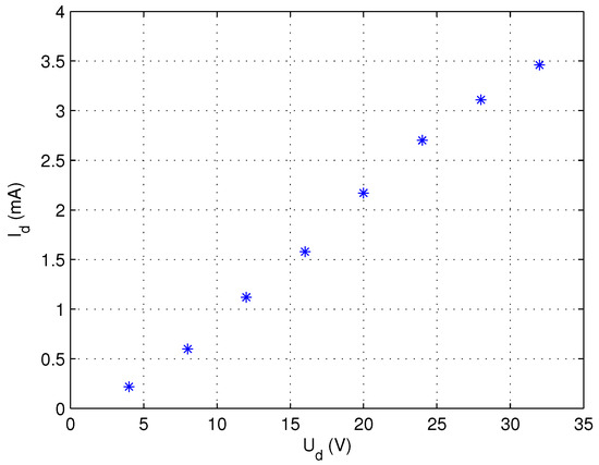
Figure 12.
relationship curve under fixed electrode spacing.
Collecting the data under different electrode spacing, the equivalent resistance corresponding to different electrode spacing can be obtained as shown by the data points in Figure 13. It can be observed that increases with the increase in D. According to (33) and (34), the relationship between and D depends on the expression of the grid cell resistance R. A power function is used to describe the variation in R with D,
where and are constants to be determined. By fitting the data points of , the value of can be obtained as 0.142.
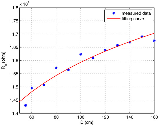
Figure 13.
Variation in with electrode spacing.
The value of can be determined by the following method: arbitrarily select a value for , denoted as , and substitute it into (37) to perform simulation. The equivalent resistance between the electrodes is obtained and compared with the measured under the same condition. Then the grid resistance parameter can be obtained as
The obtained and are put into the network for simulation, and the curve of equivalent resistance changing with D is obtained, as shown by the red curve in Figure 13. It can be seen that the variation in estimated with D is close to the actual situation.
4.3. Acquisition of Capacitance C and Fractional Order
Viewed from the electrodes, the entire water network can be equivalently represented as a parallel combination of a resistor and a fractional-order capacitor, where and denote their values, respectively, as shown in Figure 14.
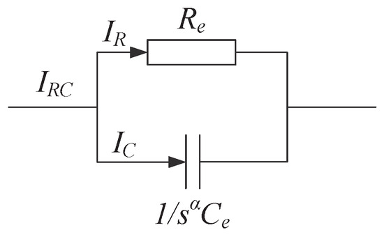
Figure 14.
Resistance-Capacitance Model.
The current flowing through a fractional-order capacitor satisfies the following equation,
The frequency characteristic of a fractional-order differentiator is
Therefore, the phase of current leading voltage is
If the capacitor is of integer order ( = 1), leads the voltage by 90 degrees. For a fractional-order capacitor, whose order is between 0 and 1, the angle by which the current leads the voltage is between 0 and 90 degree, and is proportional to the value of . In this way, the value of can be determined by measuring the phase lead of the capacitor current over the capacitor voltage.
Based on this principle, another measurement experiment is performed. AC voltage is applied to the water body through the electrodes. The measured current includes the current flowing through the resistor and capacitor ,
The schematic diagram of the charged water body measurement experiment is shown in Figure 15. The electrodes are placed in water, and the distance between the electrodes is measured. The waveforms of the voltage and are captured using an oscilloscope. The equivalent circuit of the experimental circuit is shown in Figure 16.
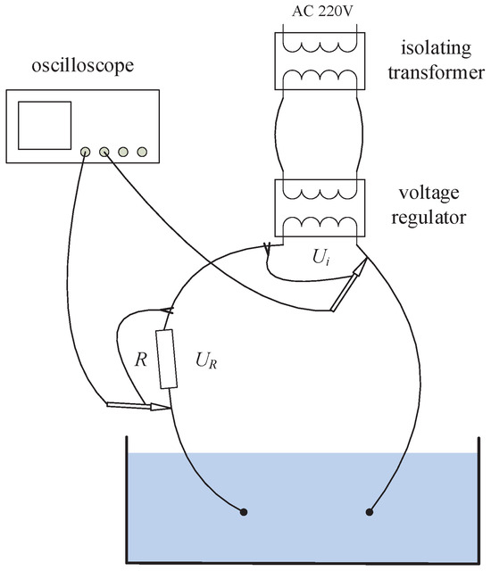
Figure 15.
Schematic diagram of the charged water body measurement experiment.
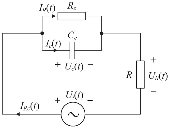
Figure 16.
Equivalent circuit of the charged water body experimental circuit.
The measured values of and are shown in Figure 17. It can be derived that , and . Since the equivalent resistance between the electrodes has been obtained through a DC voltage experiment, the current flowing through can be determined by . By subtracting the calculated from the measured total current , the current flowing through can be obtained, as illustrated in Figure 18.
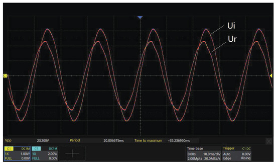
Figure 17.
Measured waveforms of voltages and under electrode spacing of 100 cm.
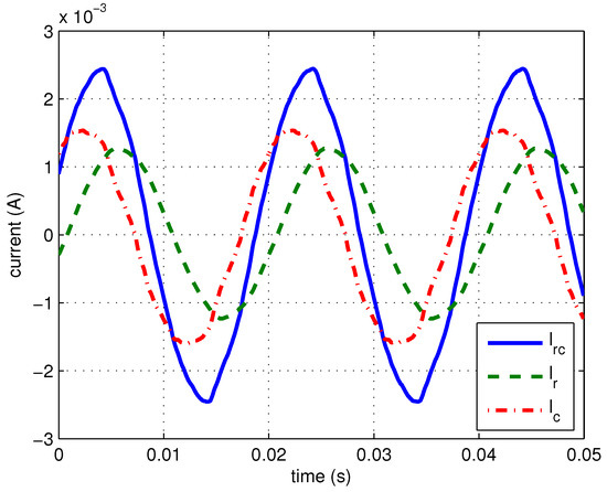
Figure 18.
Waveforms of , and under electrode spacing of 100 cm.
The phase difference between and can be obtained by phase detection algorithms. Since and are in phase, is also the phase difference between and , which can be used to estimate . The experiments are repeated for different electrode spacings to obtain phase differences. The mean phase difference is calculated for different electrode spacings, obtaining = . The fractional order is then calculated according to (41), yielding = 0.723.
Based on the currents obtained at different electrode spacings, the current amplitudes corresponding to different electrode spacings are obtained, where i = 1, 2, …, m. The current flowing through satisfies (39). As indicated by (40), the amplitude–frequency gain of the fractional-order differentiator is 20log, where is the angular frequency of the input signal. Moreover, the magnitude of is proportional to the value of . Hence the ratio of the amplitude of to that of the input voltage U is . According to the value of , , and , the value of can be calculated as
The equivalent capacitance corresponding to different electrode spacings is obtained, as shown in Figure 19. It can be observed that decreases with the increase of D. According to (35) and (36), the relationship between and D depends on the expression for the grid cell capacitance C. A power function is used to describe the variation in C with D,
where and are undetermined constants. By fitting the measured data points of , the value of can be determined as 0.1.
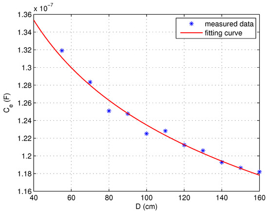
Figure 19.
Variation in with electrode spacing.
The value of can be obtained using the following method: arbitrarily select a value for , denoted as , and substitute it into Equation (44) for simulation. This yields the equivalent capacitance between electrodes, denoted as . By comparing with the measured under the same conditions, the grid capacitance parameter can be determined,
The obtained and are put into the network for simulation, and the curve of equivalent capacitance changing with D is obtained, as shown by the red curve in Figure 19. It can be seen that the variation in estimated with D is similar to the actual situation.
5. Model Verification
To validate the charged water body model proposed in this paper, the model is realized by Matlab code, and then simulation is performed to test the estimation performance under different conditions.
A sinusoidal voltage source with a peak-to-peak value of 30 V and frequency of 50 Hz is applied to perform the test. The size of the water tank is 300 cm × 200 cm × 50 cm, and the electrodes are positioned at (100, 100, 30) and (200, 100, 30) (cm), respectively. Simulation is performed and the distribution of the peak-to-peak value of AC voltage at a depth of 20 cm in the charged water body is depicted in Figure 20.
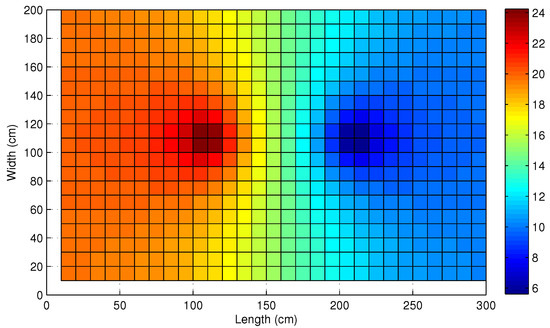
Figure 20.
The distribution of the AC voltage at a depth of 20 cm.
To validate the effectiveness of the charged water body model, the simulation results are compared with those obtained by actual experiments. Firstly, the voltage distribution of the charged water body is investigated. The experiment is performed under the same condition as applied in simulation. The measurement scheme is shown in Figure 21. Two sequences of voltage measurements are performed along the length and width of the pool, respectively, which are labeled as ➀ and ➁ in Figure 21, respectively. The spacing between adjacent measurement points is 10 cm. The depth of all the measurement points is 20 cm.
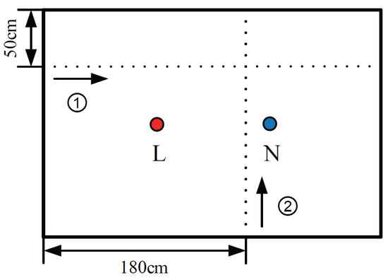
Figure 21.
The measurement scheme of the voltage distribution.
The distribution of the measured peak-to-peak voltage along the length and width of the pool are displayed as data points in Figure 22 and Figure 23, respectively. In addition, the estimated voltage distribution is also displayed in Figure 22 and Figure 23. It can be observed that the estimated voltage distribution is close to the sampled data.
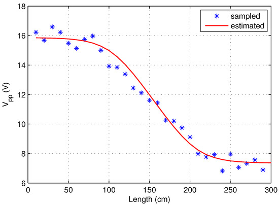
Figure 22.
The measured and estimated voltage distribution along the length.
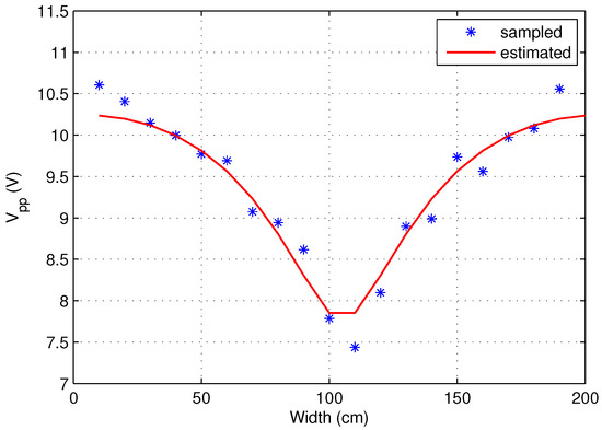
Figure 23.
The measured and estimated voltage distribution along the width.
Secondly, the leak current between the electrodes is investigated. A set of measurements are performed. The electrode spacing is set as 50 cm to 160 cm and the voltages and are recorded simultaneously. Model simulations are conducted under the same conditions, and the data collected from the experiment are compared with the data obtained from the model simulations. For example, Figure 24 and Figure 25 depict the waveforms of and obtained from the experiment and model simulation, respectively, when the electrode spacing is 50 cm.
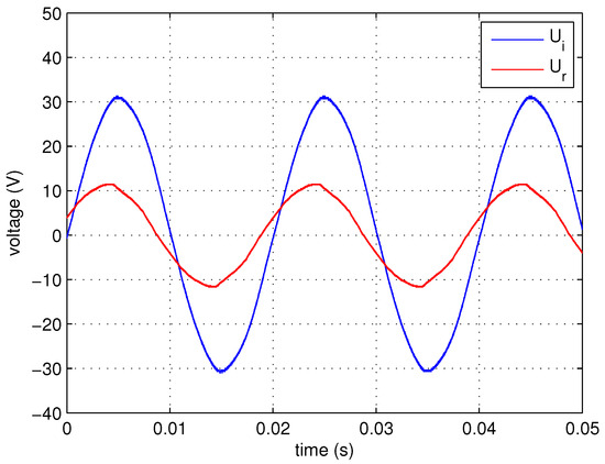
Figure 24.
Measured waveforms of voltage and under electrode spacing of 50 cm.
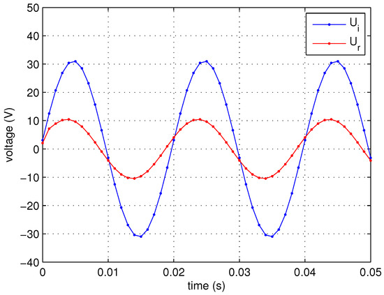
Figure 25.
Simulated waveforms of voltage and under electrode spacing of 50 cm.
The charged water body can be characterized by the amplitude of the leak current and its phase relative to input voltage . Therefore, the amplitude of the leak current and its phase lead relative to are calculated for different electrode distances. The measured and simulated amplitudes of are shown in Figure 26, and the measured and simulated phase leads of relative to are shown in Figure 27. As depicted in Figure 26 and Figure 27, the voltage amplitude and phase estimated by the model closely match the measured values in the intermediate distance range (90–150 cm), but exhibit larger deviation when the electrode distance is too small (50 cm, 60 cm, 70 cm) and too large (160 cm). This validates the model’s effectiveness within its optimal operational range.
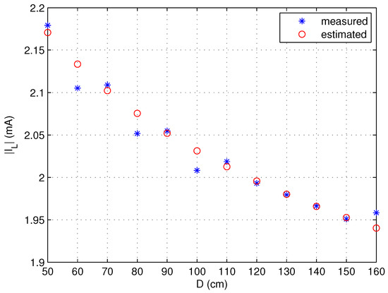
Figure 26.
The amplitudes of under different electrode spacing.
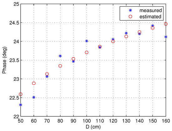
Figure 27.
The phase lead of with respect to under different electrode spacing.
6. Conclusions
A RC network-based model of a charged water body is constructed in this paper. The electrical characteristics of the charged water body are simulated by the combination of RC circuit units. The calculation method of each physical quantity is designed, and a practical method is designed to obtain parameters of the network. The effectiveness of the proposed model is verified by the experiment. Experimental results show that the proposed model can effectively reflect the electrical characteristics of the charged water body. Further investigation will be performed in the future, such as the use of a comprehensive RLC model to define the precise frequency and spatial scales at which inductive effects become significant, and performing a detailed parameter sensitivity analysis across a wider range of frequencies and water conductivities.
Author Contributions
Writing—original draft preparation, S.L.; methodology, Y.Z.; relevant experiments, W.Z.; data analysis, W.L.; writing—review and editing, M.L. All authors have read and agreed to the published version of the manuscript.
Funding
The authors declare that this study received funding from the project of China Southern Power Grid Technology Corporation (No. GDKJXM20222596). The funder was not involved in the study design, collection, analysis, interpretation of data, the writing of this article or the decision to submit it for publication.
Data Availability Statement
The datasets generated and/or analysed during the current study are not publicly available due to a confidentiality agreement.
Conflicts of Interest
Author S.L., Y.Z. and W.L. were employed by the company Foshan Power Supply Bureau, Guangdong Power Grid Co., Ltd. The remaining authors declare that the research was conducted in the absence of any commercial or financial relationships that could be construed as a potential conflict of interest.
References
- Giri, S.; Waghmode, A.; Tumram, N.K. Study of different facets of electrocution deaths: A 5-year review. Egypt. J. Forensic Sci. 2019, 9, 1. [Google Scholar] [CrossRef]
- Pongyart, N.; Somboon, T.; Weerasakul, W.; Buaprathoom, S.; Buaprathoom, J. Development of an Autonomous Robotic Boat for Localization of Electricity Leakage in Water. In Proceedings of the 2023 Research, Invention, and Innovation Congress: Innovative Electricals and Electronics (RI2C), Bangkok, Thailand, 24–25 August 2023; IEEE: Piscataway, NJ, USA, 2023; pp. 143–146. [Google Scholar]
- Kadan-Jamal, K.; Jog, A.; Sophocleous, M.; Desagani, D.; Teig-Sussholz, O.; Georgiou, J.; Avni, A.; Shacham-Diamand, Y. A study on the dielectric behaviour of plant cell suspensions using wideband electrical impedance spectroscopy (WB-EIS). In Proceedings of the 2020 IEEE SENSORS, Rotterdam, The Netherlands, 25–28 October 2020; IEEE: Piscataway, NJ, USA, 2020; pp. 1–4. [Google Scholar]
- Hlova, A.; Litynskyy, S.; Muzychuk, Y.; Muzychuk, A. Numerical solution of initial boundary-value problem for homogeneous wave equation with dynamic boundary conditions using Laguerre transform on time variable and boundary element method. In Proceedings of the 2021 IEEE 26th International Seminar/Workshop on Direct and Inverse Problems of Electromagnetic and Acoustic Wave Theory (DIPED), Tbilisi, Georgia, 8–10 September 2021; IEEE: Piscataway, NJ, USA, 2021; pp. 222–227. [Google Scholar]
- Rao, S.S. The Finite Element Method in Engineering; Elsevier: Amsterdam, The Netherlands, 2010. [Google Scholar]
- Meng, R.; Cao, L.; Zhang, Q. Study on the performance of variable-order fractional viscoelastic models to the order function parameters. Appl. Math. Model. 2023, 121, 430–444. [Google Scholar] [CrossRef]
- Grabowski, D.; Jakubowska-Ciszek, A.; Klimas, M. Fractional-Order Model of Electric Arc Furnace. IEEE Trans. Power Deliv. 2023, 38, 3761–3770. [Google Scholar] [CrossRef]
- Sun, H.; Zhang, Y.; Baleanu, D.; Chen, W.; Chen, Y. A new collection of real world applications of fractional calculus in science and engineering. Commun. Nonlinear Sci. Numer. Simulat. 2018, 64, 219–231. [Google Scholar] [CrossRef]
- Lenzi, E.; Zola, R.; Rossato, R.; Ribeiro, H.; Vieira, D.; Evangelista, L. Asymptotic behaviors of the Poisson-Nernst-Planck model, generalizations and best adjust of experimental data. Sci. Rep. 2017, 226, 40–45. [Google Scholar] [CrossRef]
- Rasoolzadeh, A.; Hashemi, S.A.; Pahlevani, M. A fractional-order state estimation method for supercapacitor energy storage. Electronics 2025, 14, 3231. [Google Scholar] [CrossRef]
- Fouda, M.; Elwakil, A.; Radwan, A.; Allagui, A. Power and energy analysis of fractional-order electrical energy storage devices. Energy 2016, 111, 785–792. [Google Scholar] [CrossRef]
- Elwakil, A.; Radwan, A.; Freeborn, T.; Allagui, A.; Maundy, B.; Fouda, M. Low-voltage commercial super-capacitor response to periodic linear-with-time current excitation: A case study. IET Circ. Dev. Syst. 2017, 11, 189–195. [Google Scholar] [CrossRef]
- Zhang, Q.; Wei, K. A comparative study of fractional-order models for supercapacitors in electric vehicles. Int. J. Electrochem. Sci. 2024, 19, 100441. [Google Scholar] [CrossRef]
- Podlubny, I. Fractional Differential Equations; Academic Press: New York, NY, USA, 1999. [Google Scholar]
- Fu, B.; Freeborn, T. Electrical equivalent network modeling of forearm tissue bioimpedance. In Proceedings of the 2019 SoutheastCon, Huntsville, AL, USA, 11–14 April 2019; IEEE: Piscataway, NJ, USA, 2019; pp. 1–7. [Google Scholar]
- Aouane, S.; Claverie, R.; Techer, D.; Durickovic, I.; Rousseau, L.; Poulichet, P.; Francais, O. Cole-Cole parameter extraction from electrical impedance spectroscopy for real-time monitoring of vegetal tissue: Case study with a single celery stalk. In Proceedings of the 2021 International Workshop on Impedance Spectroscopy (IWIS), Chemnitz, Germany, 9 September–1 October 2021; IEEE: Piscataway, NJ, USA, 2021; pp. 48–51. [Google Scholar]
- AboBakr, A.; Mohsen, M.; Said, L.A.; Madian, A.H.; Elwakil, A.S.; Radwan, A.G. Banana ripening and corresponding variations in bio-impedance and glucose levels. In Proceedings of the 2019 Novel Intelligent and Leading Emerging Sciences Conference (NILES), Giza, Egypt, 28–30 October 2019; IEEE: Piscataway, NJ, USA, 2019; Volume 1, pp. 130–133. [Google Scholar]
- Mahata, S.; Ghosh, A.; Kar, R.; Mandal, D.; Saha, S. Approximation of fractional order wood tissue impedance model using flower pollination algorithm. In Proceedings of the 2018 15th International Conference on Electrical Engineering/Electronics, Computer, Telecommunications and Information Technology (ECTI-CON), Chiang Rai, Thailand, 18–21 July 2018; IEEE: Piscataway, NJ, USA, 2018; pp. 664–667. [Google Scholar]
- Aboalnaga, B.M.; Said, L.A.; Madian, A.H.; Elwakil, A.S.; Radwan, A.G. Cole Bio-Impedance Model Variations in Daucus Carota Sativus Under Heating and Freezing Conditions. IEEE Access 2019, 7, 113254–113263. [Google Scholar] [CrossRef]
- Chen, Y. Impulse Response Invariant Discretization of Fractional Order Integrators/Differentiators. Filter Design and Analysis, MATLAB Central. 2008. Available online: http://www.mathworks.com/matlabcentral/fileexchange/21342-impulse-response-invariant-discretization-of-fractional-order-integrators-differentiators (accessed on 22 September 2025).
- Simić, M.; Freeborn, T.J.; Veletić, M.; Seoane, F.; Stojanović, G.M. Parameter Estimation of the Single-Dispersion Fractional Cole-Impedance Model With the Embedded Hardware. IEEE Sens. J. 2023, 23, 12978–12987. [Google Scholar] [CrossRef]
- De Santis, V.; Martynyuk, V.; Lampasi, A.; Fedula, M.; Ortigueira, M.D. Fractional-order circuit models of the human body impedance for compliance tests against contact currents. AEU-Int. J. Electron. Commun. 2017, 78, 238–244. [Google Scholar] [CrossRef]
Disclaimer/Publisher’s Note: The statements, opinions and data contained in all publications are solely those of the individual author(s) and contributor(s) and not of MDPI and/or the editor(s). MDPI and/or the editor(s) disclaim responsibility for any injury to people or property resulting from any ideas, methods, instructions or products referred to in the content. |
© 2025 by the authors. Licensee MDPI, Basel, Switzerland. This article is an open access article distributed under the terms and conditions of the Creative Commons Attribution (CC BY) license (https://creativecommons.org/licenses/by/4.0/).