

Innovative Machine Learning and Image Processing Methodology for Enhanced Detection of Aleurothrixus Floccosus
 , , , ,
  ,
,  and
and 
Abstract
1. Introduction
2. Background Definitions
2.1. Grayscale
2.2. Equalization
2.3. Median Filter
2.4. Salt and Pepper Noise
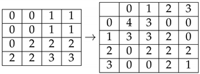
2.5. GLCM Matrix
2.6. Data Augmentation
3. Materials and Methods
3.1. Methodology
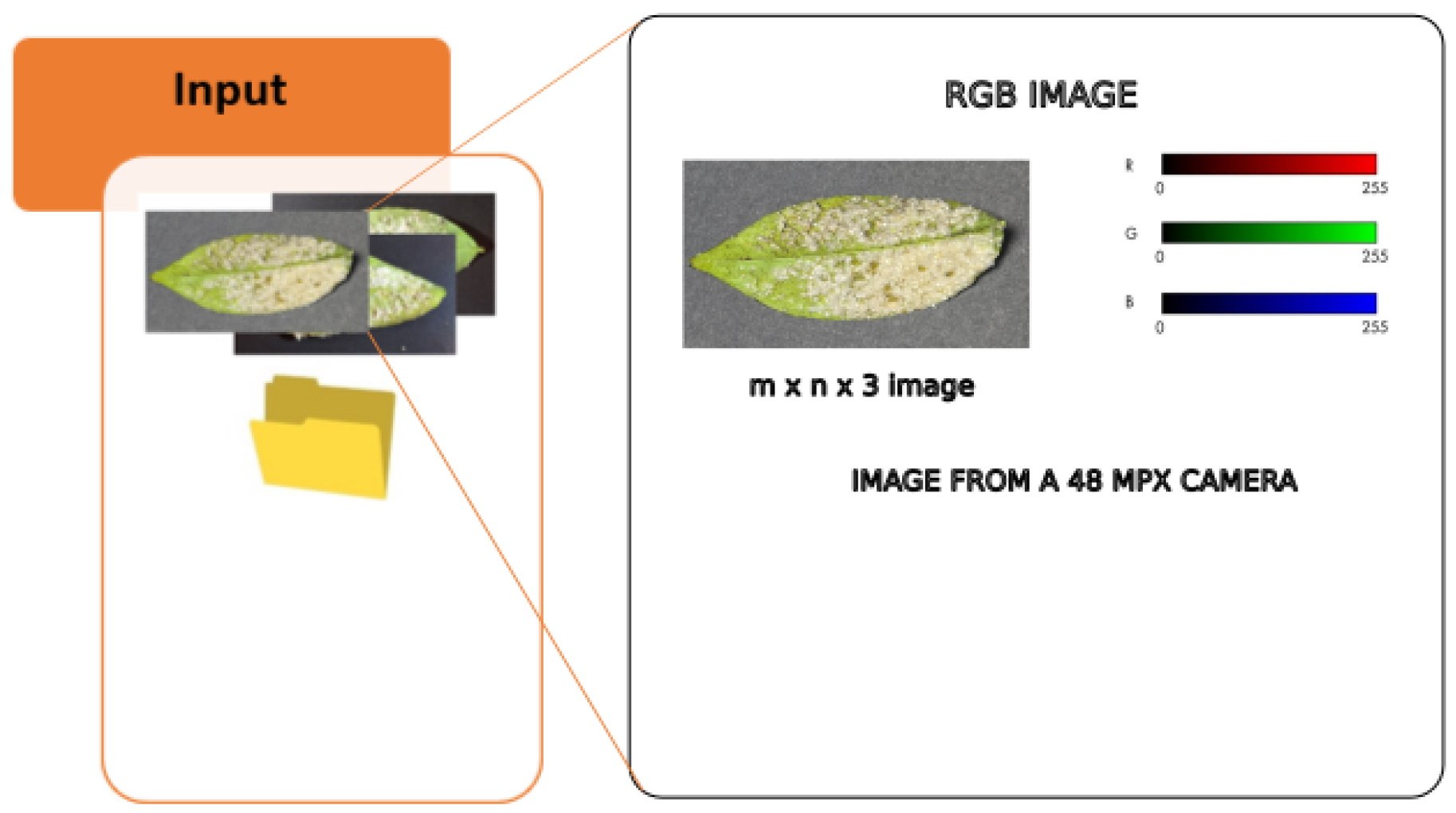
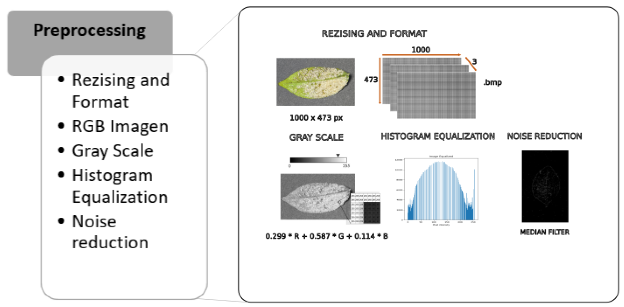
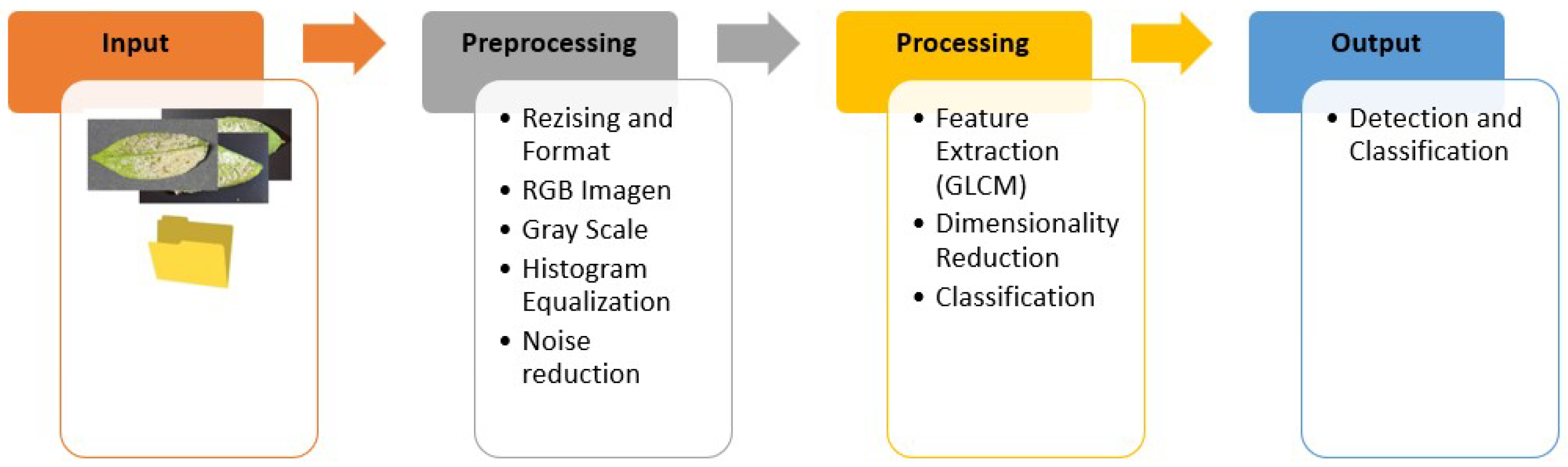
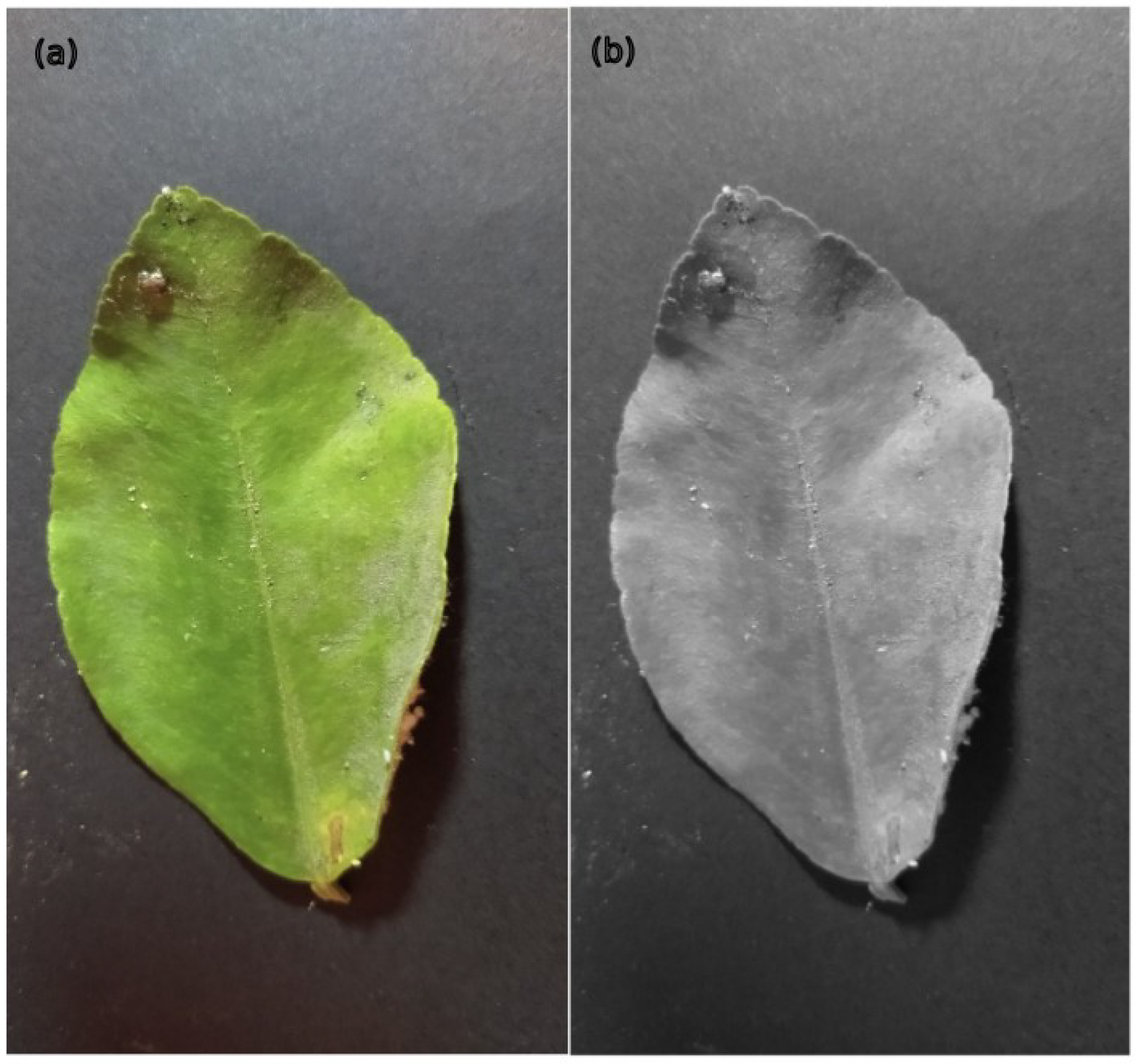
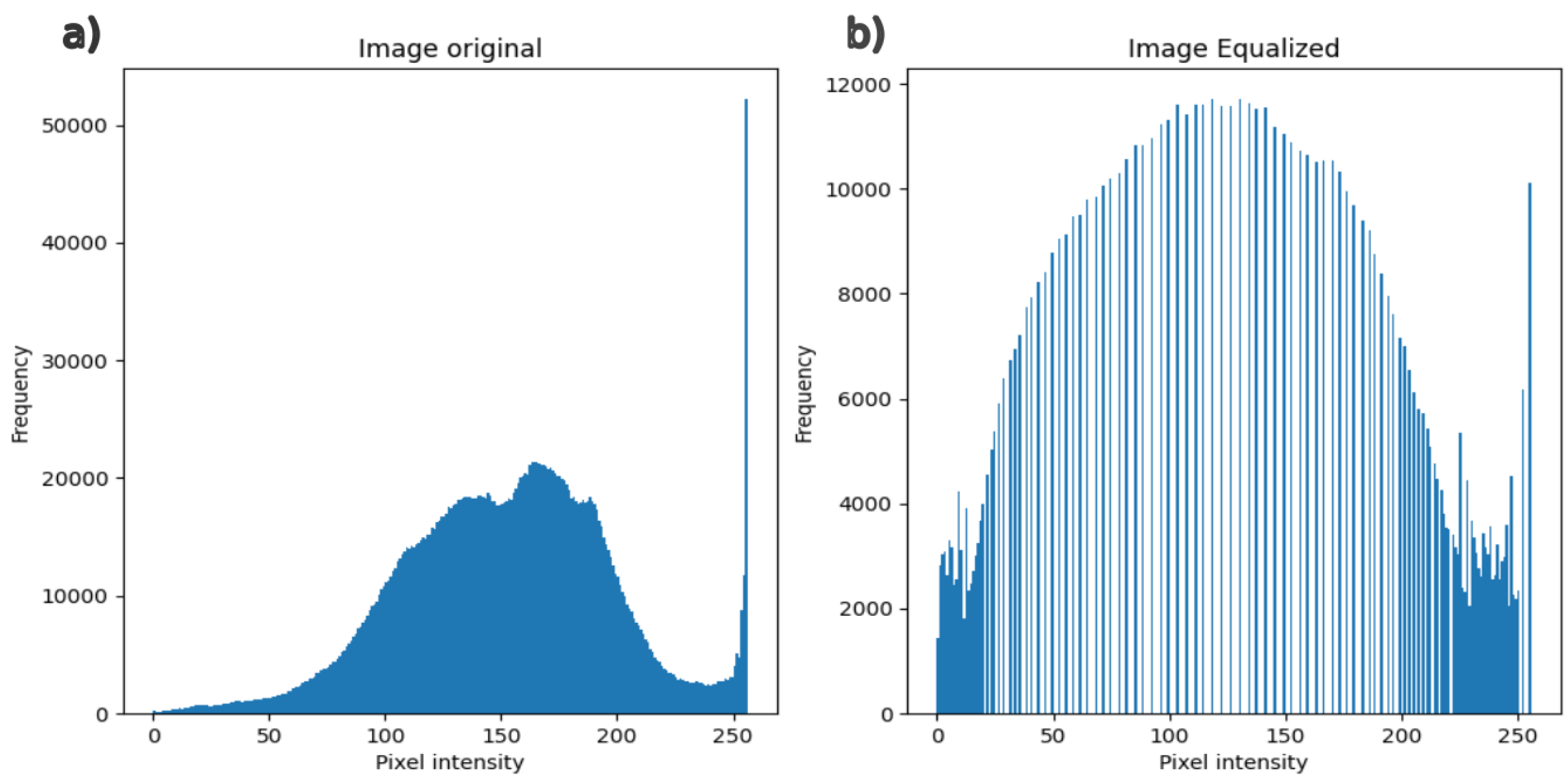
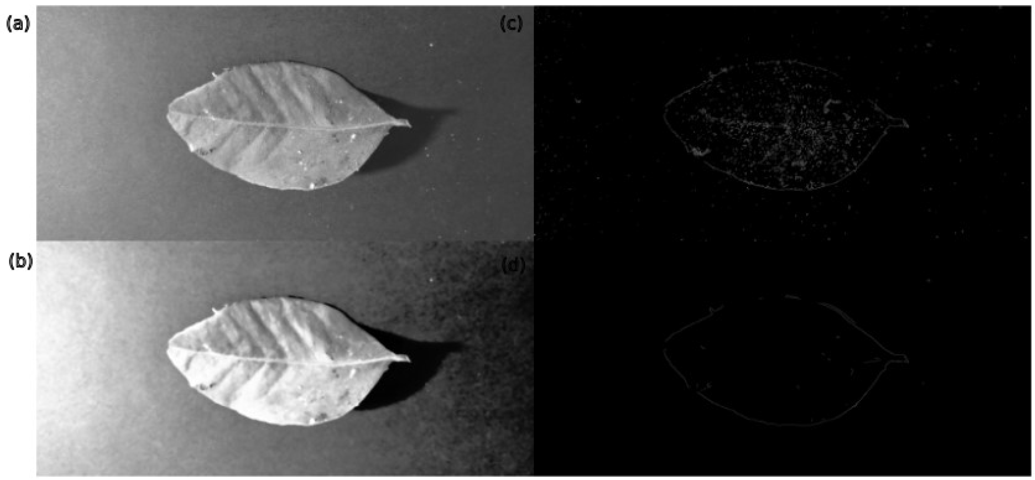
- Preprocessing: We transform the obtained RGB image, which is composed of three channels, into a single grayscale image for subsequent equalization. This process redistributes pixel intensity improving contrast. Finally, we apply noise reduction using a median filter to remove unwanted noise from the image.Figure 3. Methodology—Preprocessing.
![Electronics 14 00358 g003]()
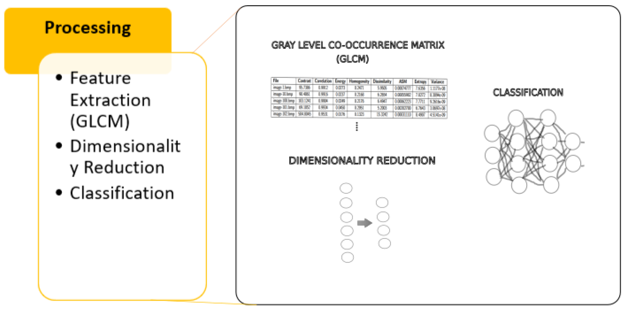
- Processing: We apply dimensionality reduction to simplify the dataset while preserving as much relevant information as possible, data augmentation to balance the obtaned images and finally classify using algorithms such as SVM, DECISION TREE, and XGBoost.Figure 4. Methodology—Processing.
![Electronics 14 00358 g004]()
3.2. Data Description
3.3. Image Preprocessing
3.3.1. Image Type and Size
3.3.2. Transform
3.3.3. Histogram Equalization with the n CDF (Cumulative Distribution Function)
3.3.4. Noise Reduction
3.4. Image Processing
3.4.1. Feature Extraction
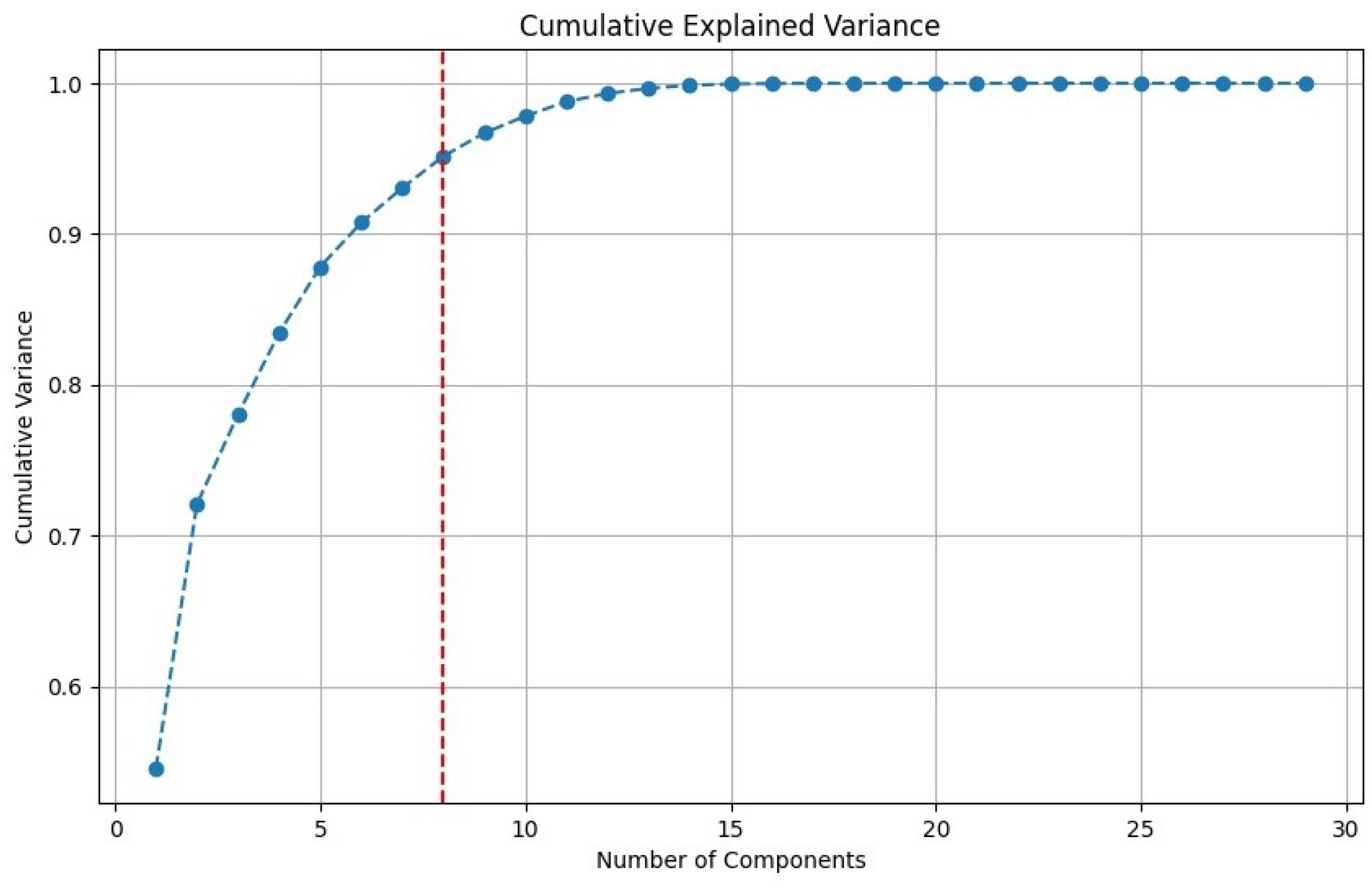
3.4.2. Dimensionality Reduction
3.4.3. Classification Algorithms
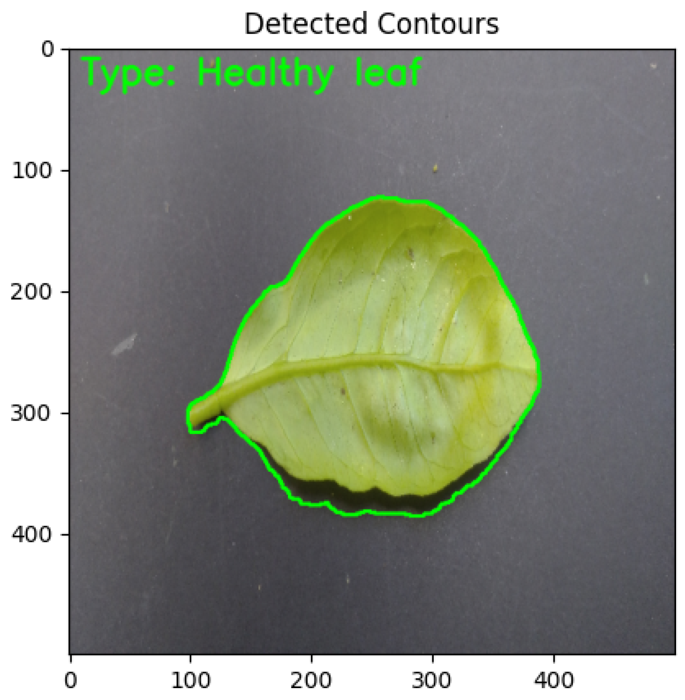
3.4.4. Segmentation
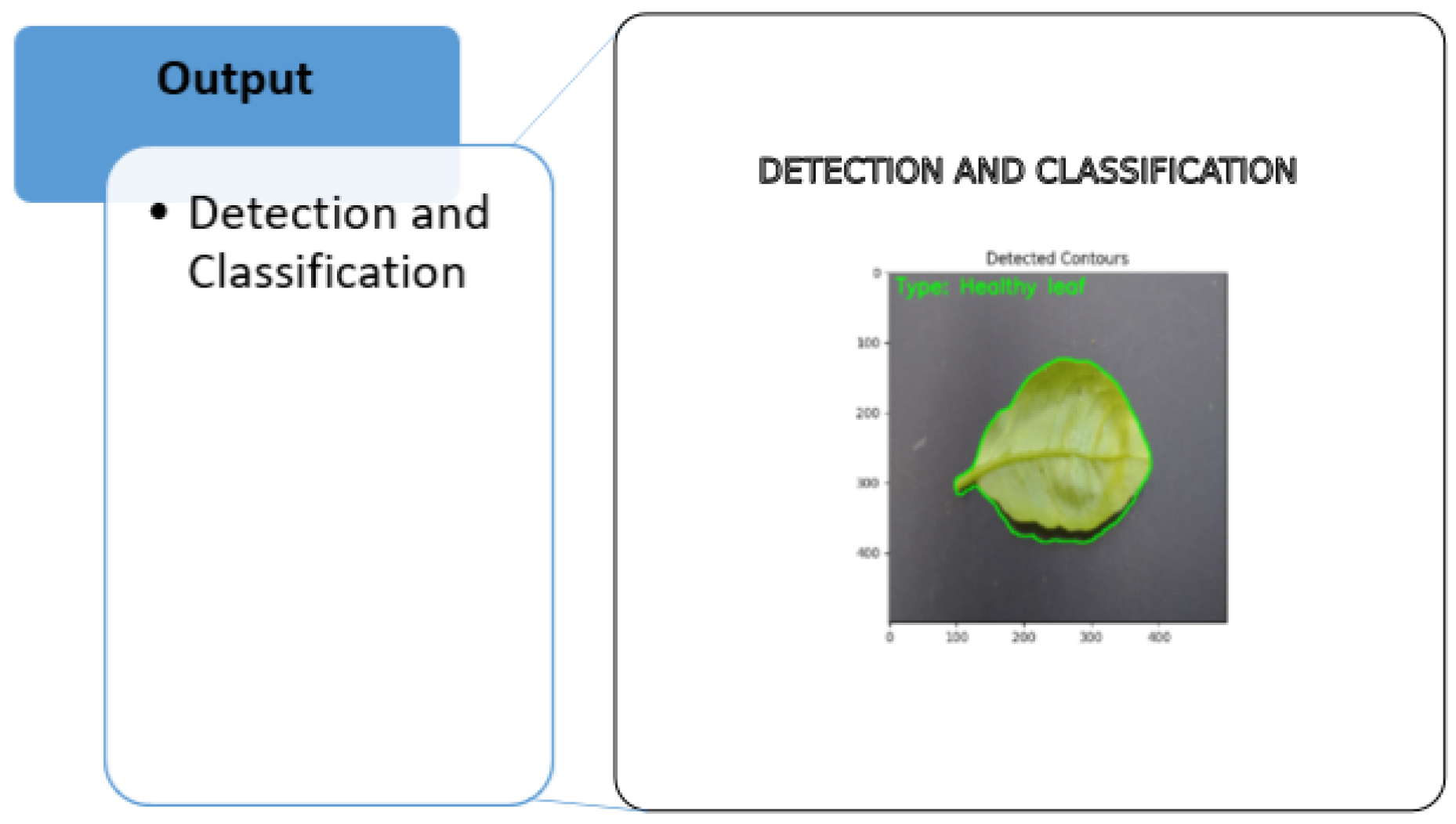
3.4.5. Detection and Classification
4. Results and Discussions
4.1. Pre-Processing
4.2. Processing
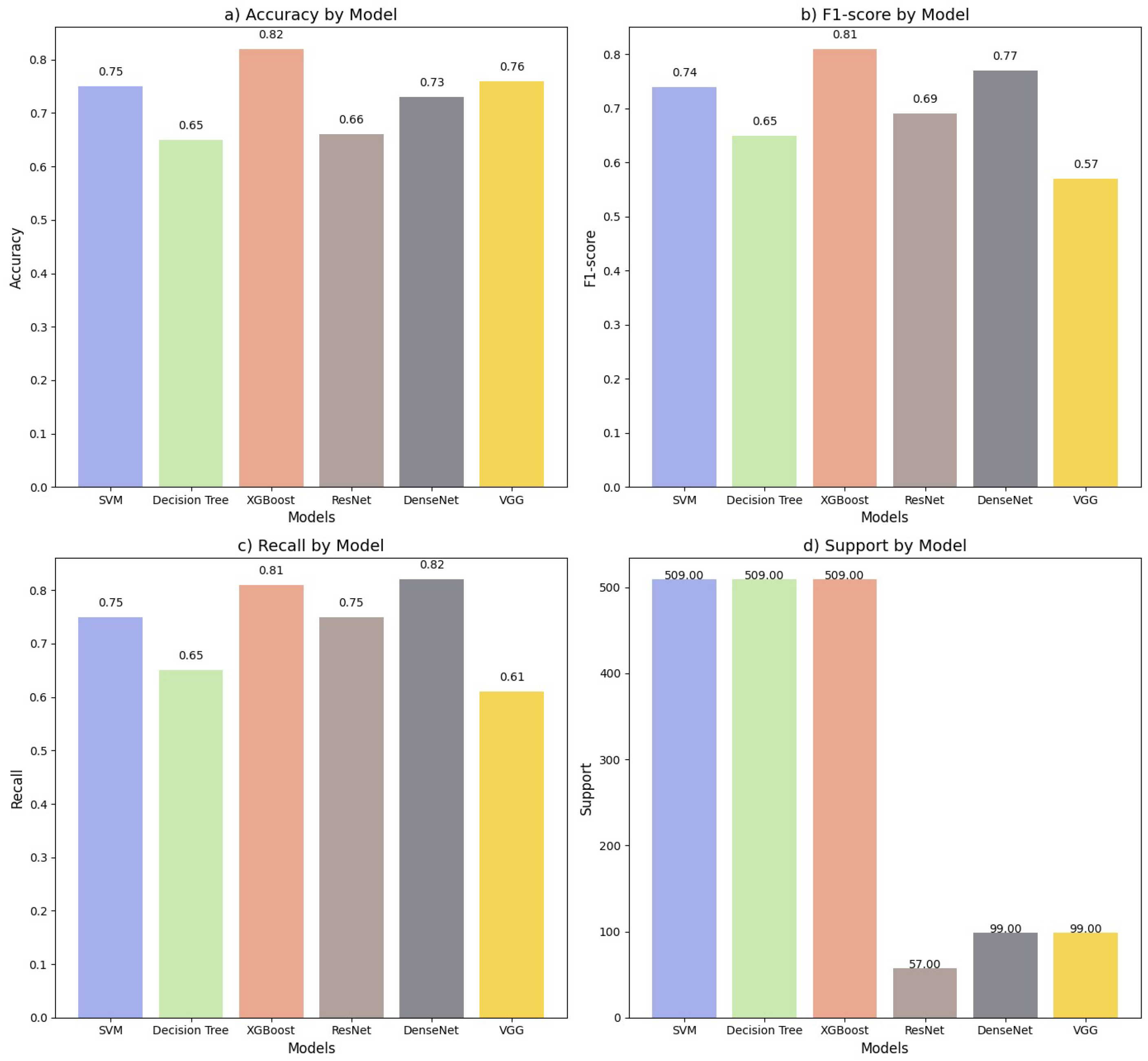
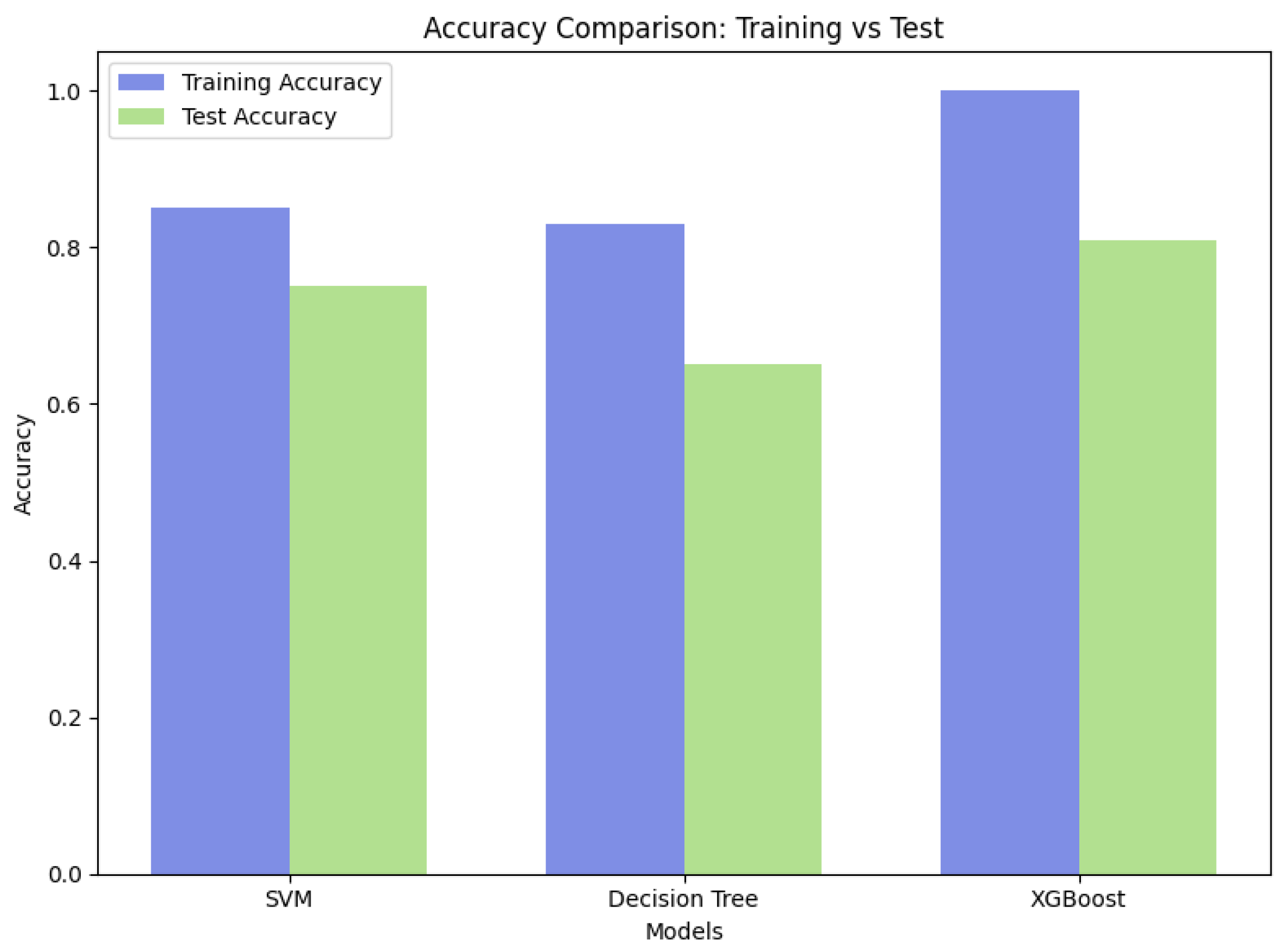
4.3. Classification
5. Conclusions
Author Contributions
Funding
Data Availability Statement
Acknowledgments
Conflicts of Interest
Abbreviations
| GLCM | Gray level co-occurrence matrices |
| GLM | General linear model |
| CDF | Cumulative Distribution Function |
| SVM | Support Vector Machine |
| IoT | Internet of Things |
| WSN | Wireless sensor networks |
| CNN | Convolutional Neural Networks |
| DenseNet | Dense convolutional network |
| ANOVA | Analysis of variance |
| RGB | Red Green Blue |
References
- Luo, D.; Xue, Y.; Deng, X.; Yang, B.; Chen, H.; Mo, Z. Citrus Diseases and Pests Detection Model Based on Self-Attention YOLOV8. IEEE Access 2023, 11, 139872–139881. [Google Scholar] [CrossRef]
- Hachimi, C.E.; Belaqziz, S.; Khabba, S.; Sebbar, B.; Dhiba, D.; Chehbouni, A. Smart Weather Data Management Based on Artificial Intelligence and Big Data Analytics for Precision Agriculture. Agriculture 2023, 13, 95. [Google Scholar] [CrossRef]
- Dhaka, V.S.; Meena, S.V.; Rani, G.; Sinwar, D.; Kavita, I.M.F.; Wozniak, M. A survey of deep convolutional neural networks applied for prediction of plant leaf diseases. Sensors 2021, 21, 4749. [Google Scholar] [CrossRef] [PubMed]
- Elbasi, E.; Mostafa, N.; Alarnaout, Z.; Zreikat, A.I.; Cina, E.; Varghese, G. Artificial Intelligence Technology in the Agricultural Sector: A Systematic Literature Review. IEEE Access 2023, 11, 171–202. [Google Scholar] [CrossRef]
- Choudhury, S.; Singh, R.; Gehlot, A.; Kuchhal, P.; Akram, S.V.; Priyadarshi, N.; Khan, B. Agriculture Field Automation and Digitization Using Internet of Things and Machine Learning. J. Sens. 2022, 2022, 9042382. [Google Scholar] [CrossRef]
- Akhter, R.; Sofi, S.A. Precision agriculture using IoT data analytics and machine learning. J. King Saud-Univ. Comput. Inf. Sci. 2022, 234, 5602–5618. [Google Scholar] [CrossRef]
- Abdu, A.M.; Mokji, M.M.; Sheikh, U.U. Machine learning for plant disease detection: An investigative comparison between support vector machine and deep learning. IAES Int. J. Artif. Intell. 2020, 9, 670–683. [Google Scholar] [CrossRef]
- Li, L.; Zhang, S.; Wang, B. Plant Disease Detection and Classification by Deep Learning—A Review. IEEE Access 2021, 9, 56683–56698. [Google Scholar] [CrossRef]
- Hosny, K.M.; El-Hady, W.M.; Samy, F.M.; Vrochidou, E.; Papakostas, G.A. Multi-Class Classification of Plant Leaf Diseases Using Feature Fusion of Deep Convolutional Neural Network and Local Binary Pattern. IEEE Access 2023, 11, 62307–62317. [Google Scholar] [CrossRef]
- Shireesha, G.; Reddy, B.E. Citrus Fruit and Leaf Disease Detection Using DenseNet. In Proceedings of the 2022 International Conference on Smart Generation Computing, Communication and Networking (SMART GENCON), Bangalore, India, 23–25 December 2022; pp. 1–5. [Google Scholar]
- Mahmoudi, A.; Benfekih, L.A.; Yigit, A.; Goosen, M.F.A. An assessment of population fluctuations of citrus pest woolly whitefly Aleurothrixus floccosus (Maskell, 1896) (Homoptera, Aleyrodidae) and its parasitoid Cales noacki Howard, 1907 (Hymenoptera, Aphelinidae): A case study from Northwestern Algeria. Acta Agric. Slov. 2018, 111, 407–417. [Google Scholar] [CrossRef]
- Vélez Serrano, J.F. Vision por Computador; Chapter 3; Paraninfo: Madrid, Spain, 2021; p. 72. [Google Scholar]
- Jain, A.K. Fundamentals of Digital Processing; Prentice-Hall: Upper Saddle River, NJ, USA, 1989. [Google Scholar]
- Kumar, A.; Rout, K.N.; Kumar, S. High Density Salt and Pepper Noise Removal by a Threshold Level Decision based Mean Filter. In Proceedings of the 2018 International Conference on Applied Electromagnetics, Signal Processing and Communication (AESPC), Bhubaneswar, India, 22–24 October 2018; Volume 1, pp. 1–5. [Google Scholar]
- Gárate-Escamila, A.K.; El Hassani, A.H.; Andrès, E. Classification models for heart disease prediction using feature selection and PCA. Inform. Med. Unlocked 2020, 19, 100330. [Google Scholar] [CrossRef]
- Alazawi, S.A.; Shati, N.M.; Abbas, A.F. Texture features extraction based on GLCM for face retrieval system. Period. Eng. Nat. Sci. 2019, 7, 1459–1467. [Google Scholar] [CrossRef]
- Kim, Y.; Uddin, A.F.M.S.; Bae, S.H. Local Augment: Utilizing Local Bias Property of Convolutional Neural Networks for Data Augmentation. IEEE Access 2021, 9, 15191–15199. [Google Scholar] [CrossRef]
- Hong, W.; Chen, J.; Chang, P.S.; Wu, J.; Chen, T.S.; Lin, J. A Color Image Authentication Scheme With Grayscale Invariance. IEEE Access 2021, 9, 6522–6535. [Google Scholar] [CrossRef]
- Chen, R.C.; Dewi, C.; Zhuang, Y.C.; Chen, J.K. Contrast Limited Adaptive Histogram Equalization for Recognizing Road Marking at Night Based on Yolo Models. IEEE Access 2023, 11, 92926–92942. [Google Scholar] [CrossRef]
- Van Griethuysen, J.J.; Fedorov, A.; Parmar, C.; Hosny, A.; Aucoin, N.; Narayan, V.; Beets-Tan, R.G.; Fillion-Robin, J.C.; Pieper, S.; Aerts, H.J. Computational radiomics system to decode the radiographic phenotype. Cancer Res. 2017, 77, e104–e107. [Google Scholar] [CrossRef]
- Riyana Putri Putri, F.N.; Wibowo, N.C.; Mustofa, H. Clustering of Tuberculosis and Normal Lungs Based on Image Segmentation Results of Chan-Vese and Canny with K-Means. Indones. J. Artif. Intell. Data Min. 2023, 6, 18–28. [Google Scholar] [CrossRef]


 |
| Principal Components | Variance | Variance (%) |
|---|---|---|
| PC1 | 0.274846 | 57.372779 |
| PC2 | 0.088262 | 18.424324 |
| PC3 | 0.029825 | 6.225807 |
| PC4 | 0.027170 | 5.671614 |
| PC5 | 0.022058 | 4.604421 |
| PC6 | 0.014767 | 3.082623 |
| PC7 | 0.011572 | 2.415664 |
| PC8 | 0.010552 | 2.202767 |
| PC1 | PC2 | PC3 | PC4 | PC5 | PC6 | PC7 | PC8 | |
|---|---|---|---|---|---|---|---|---|
| Energy | 0.330514 | 0.060444 | 0.008409 | −0.047678 | −0.066937 | −0.004838 | −0.050243 | −0.027284 |
| Variance_Sum | 0.277826 | 0.044041 | 0.022526 | −0.074000 | −0.184435 | 0.013523 | 0.051554 | −0.015736 |
| Variance | 0.277826 | 0.044041 | 0.022526 | −0.074000 | −0.184435 | 0.013523 | 0.051554 | −0.015736 |
| Homogeneity_2 | 0.277826 | 0.044041 | 0.022526 | −0.074000 | −0.184435 | 0.013523 | 0.051554 | −0.015736 |
| Sum_Squares | 0.277826 | 0.044041 | 0.022526 | −0.074000 | −0.184435 | 0.013523 | 0.051554 | −0.015736 |
Disclaimer/Publisher’s Note: The statements, opinions and data contained in all publications are solely those of the individual author(s) and contributor(s) and not of MDPI and/or the editor(s). MDPI and/or the editor(s) disclaim responsibility for any injury to people or property resulting from any ideas, methods, instructions or products referred to in the content. |
© 2025 by the authors. Licensee MDPI, Basel, Switzerland. This article is an open access article distributed under the terms and conditions of the Creative Commons Attribution (CC BY) license (https://creativecommons.org/licenses/by/4.0/).
Share and Cite
Valderrama Solis, M.A.; Valenzuela Nina, J.; Echaiz Espinoza, G.A.; Yanyachi Aco Cardenas, D.D.; Villanueva, J.M.M.; Salazar, A.O.; Villarreal, E.R.L. Innovative Machine Learning and Image Processing Methodology for Enhanced Detection of Aleurothrixus Floccosus. Electronics 2025, 14, 358. https://doi.org/10.3390/electronics14020358
Valderrama Solis MA, Valenzuela Nina J, Echaiz Espinoza GA, Yanyachi Aco Cardenas DD, Villanueva JMM, Salazar AO, Villarreal ERL. Innovative Machine Learning and Image Processing Methodology for Enhanced Detection of Aleurothrixus Floccosus. Electronics. 2025; 14(2):358. https://doi.org/10.3390/electronics14020358
Chicago/Turabian StyleValderrama Solis, Manuel Alejandro, Javier Valenzuela Nina, German Alberto Echaiz Espinoza, Daniel Domingo Yanyachi Aco Cardenas, Juan Moises Mauricio Villanueva, Andrés Ortiz Salazar, and Elmer Rolando Llanos Villarreal. 2025. "Innovative Machine Learning and Image Processing Methodology for Enhanced Detection of Aleurothrixus Floccosus" Electronics 14, no. 2: 358. https://doi.org/10.3390/electronics14020358
APA StyleValderrama Solis, M. A., Valenzuela Nina, J., Echaiz Espinoza, G. A., Yanyachi Aco Cardenas, D. D., Villanueva, J. M. M., Salazar, A. O., & Villarreal, E. R. L. (2025). Innovative Machine Learning and Image Processing Methodology for Enhanced Detection of Aleurothrixus Floccosus. Electronics, 14(2), 358. https://doi.org/10.3390/electronics14020358