Article

A Study on Reducing the Noise Using the Kalman Filter in Digital Holographic Microscopy (DHM)

1
Graduate School of Computer Science and Systems Engineering, Kyushu Institute of Technology, 680-4 Kawazu, Iizuka-shi 820-8502, Fukuoka, Japan
2
School of ICT, Robotics, and Mechanical Engineering, Hankyong National University, IITC, 327 Chungang-ro, Anseong 17579, Kyonggi-do, Republic of Korea
*
Authors to whom correspondence should be addressed.
These authors contributed equally to this work.
Electronics 2025, 14(2), 338; https://doi.org/10.3390/electronics14020338
Submission received: 10 December 2024 / Revised: 9 January 2025 / Accepted: 15 January 2025 / Published: 16 January 2025
(This article belongs to the Special Issue Machine Learning and Deep Learning Based Pattern Recognition)

Abstract

:
Digital Holographic Microscopy (DHM) is a technique that uses the phase information of light to generate a three-dimensional (3D) profile of an object. Recently, it has been utilized in various fields such as disease diagnosis and research on microorganisms. In the process in DHM, a narrow region around one of the sidebands from the frequency domain is windowed to avoid noise caused by the direct current (DC) term. However, it may not obtain the high-frequency information about the object. On the other hand, windowing a wide region increases the noise caused by the DC term, and generates the noise in the 3D profile. To solve this trade-off, we propose a noise reduction method using Kalman filter. From the recorded hologram image, we can create the frequency domain. It obtains multiple windowed sidebands centered on multiple pixels at random from the frequency domain. This creates a group of data in which noise is generated randomly. This is regarded as frequency series data, and Kalman filtering is performed. This method can reduce the noise caused by the DC term while acquiring high-frequency information. In addition, this method has the advantage that only one image is needed for frequency series data in the Kalman filter. The effectiveness of the proposed method is verified by comparison with conventional filtering methods and general image processing methods. The validation results prove the usefulness of the proposed method, and the proposed method is expected to have a significant effect on improving the accuracy of disease diagnosis techniques using DHM.

1. Introduction

Electronics and biotechnology have recently been highly developed and active in various fields [1,2,3,4,5,6,7,8,9,10,11,12,13]. Among other things, the high demand for the early detection, diagnosis, and treatment of diseases in the medical field has led to a growing need for microscopic imaging technology. The optical microscope is one of the most useful instruments. However, optical microscopes can only record two-dimensional (2D) information. Thus, the height information of the cell is lost.
In 1948, Dennis Gabor proposed holography [14]. Specifically, holography using image sensors is called digital holography, which was proposed by Joseph W. Goodman in 1967 [15]. Since then, the technological development of digital holography has accelerated, producing many technologies that support the human life, such as 3D image visualization [16,17], object recognition [18,19], image encryption [20,21], surface profiling [22], interferometry [23], and Digital Holographic Microscopy (DHM) [14]. DHM has attracted attention in current disease diagnosis and microbiological research. While a traditional microscope provides 2D information of the object, three-dimensional (3D) information of the object can be obtained by this technology. DHM utilizes holography technology, which uses the coherence of light to record and reproduce the amplitude and the phase distributions of 3D objects by interfering and diffracting light [8,9,10,11,12,13,24,25,26,27,28,29,30,31]. DHM has produced several technologies that support our daily lives. Because of its ability to obtain 3D information from micro-objects, DHM is used in a wide range of fields, including microstructure analysis [29], microbiological research [30], and disease diagnosis using cell analysis [8,9,10,11,12,13,24,25,26,27,28]. In the medical field, it is used to diagnose the disease in which changes in the cell shape are observed, such as malaria [12] and sickle cell disease [13]. In recent years, techniques for disease diagnosis using deep learning technologies have been studied [1,2,3,4,5,6,7,8,9,10,11,12,13]. These studies aim to analyze the statistical data of 3D Profile for quick and easy disease diagnosis. Therefore, the accuracy of the data are a very important item and prerequisite. There is also research into the use of red blood cell (RBC) data to diagnose COVID-19, which had a significant impact in 2019 [10]. For example, COVID-19 shows no significant differences between the RBCs of positive and negative individuals, making the visual distinction difficult. It uses deep learning techniques to identify the instant errors in the cell height information due to diseases. This technology has the potential to significantly improve the technology of the disease diagnosis, and to enable the diagnosis of diseases that could not be diagnosed as before. The key data for diagnosis by deep learning technology must be detailed and have accurate height information. For obtaining accurate and detailed height information, the area of the windowed sideband (WS) increases to maximize the detailed 3D information of the object when extracting the sidebands from the frequency domain needs. However, since not only the sidebands, but also the direct current (DC) term, are widely distributed in the frequency domain of the recorded hologram image, the information of the DC term overlaps with the high-frequency information. As a result, the information of the DC term appears as the noise in the reconstructed 3D profile. This noise can be prevented by reducing the size of the WS. Recently, the research on disease diagnosis by DHM utilize the information obtained from narrow sidebands [8,9,10]. To that extent, the cell shape is approximated to the lower frequency, and the detailed information is lost. Cells that can be diagnosed using this technique are often those with large changes in the shape, and can be visually recognized. On the other hand, the diagnosis of the visually unidentifiable changes, such as COVID-19, may be difficult.
To solve this trade-off and produce the data for improved disease diagnosis, a new noise reduction method using the Kalman filter in DHM is proposed in this research. The Kalman filter was proposed by Rudolph E. Kalman in 1960 [32]. The Kalman filter is widely used for the accurate object location estimation and the fault diagnosis [33,34]. The traditional Kalman filter requires multiple images or videos to create time series data. Our method creates multiple data from a single recorded hologram image to create the time series data, reducing the time required to prepare the data. Our method maximizes the area of the WS of the frequency domain to obtain detailed information, and removes the noise by the Kalman filter. This allows for the detailed information to be obtained without noise. We set the maximum area of the WS in the frequency domain and obtain multiple WSs centered on multiple pixels randomly in the area. We can create the time series data from these multiple WSs. For this reason, we have to change the name of the time series to the frequency series. The frequency series data in noise is generated randomly. The Kalman filter is performed for these data to obtain the shape of the object with the reduced noise. It can obtain even the detailed shape of the object. This method can be used for other micro-objects, as long as they can be recorded by DHM. In this research, an artificial object, the microsphere, was used as 3D object of observation. The 3D profiles obtained with the traditional DHM and the proposed methods are compared with the ideal shape of the microsphere to verify the noise removal effect. The effectiveness of filtering is then verified by comparing 3D profiles of RBCs created using the proposed method with conventional methods.
The organization of the paper is as follows. Section 2 describes the principles of DHM, image processing processes in DHM and the proposed method in this research. Section 3 describes the experimental setup, and shows the experimental results. Finally, we present the conclusions in Section 4.

2. Theory

2.1. Digital Holographic Microscopy (DHM)

As we mentioned earlier, DHM uses digital holography technology to reconstruct the 3D profile of the object. Digital holography uses the coherence of light, such as a laser, which allows the phase information of light to be recorded by an image sensor. Normally, image sensors cannot record the phase of light. In digital holography, two lights are superimposed on the imaging plane to generate the interference fringes. These interference fringes can be captured by the image sensor to obtain the information on the phase.
DHM divides the coherent light into the reference and the object beams, and interferes with them. In this research, we indicate the recorded hologram image to I H o , and this is represented by Equation (1) [25,26,27,28,29],
I H o = | R | 2 + | O | 2 + R * O + R O *
where R is the complex amplitude of the reference beam, O is the complex amplitude of the object beam, and R * and O * are the complex conjugates of R and O , respectively. In Equation (1), | R | 2 + | O | 2 represents the DC term and R * O + R O * represents the real and imaginary sidebands in the frequency domain of the recorded hologram. Equation (1) can be rewritten as Equation (2) [25,26,27,28,29],
I H o = | R | 2 + | O | 2 + R * O e j ϕ + R O * e j ϕ
where ϕ represents the phase information of the recorded hologram. The components of Equation (2) are distributed in the frequency domain, as shown in Figure 1.
Figure 1a,b show the frequency domain and its cross section. The + f o and f o in Figure 1b represent R * O e j ϕ and R * O e j ϕ in Equation (2). As the sidebands are point symmetrical with respect to the center of the image, it is sufficient to focus on the one sideband and obtain the phase information of the recorded hologram. Holograms with the object information are called the object images, and holograms without the object information are called the reference images. Phase information is obtained from the recorded holograms by distinguishing between the real and imaginary parts of the image. Splitting into real and imaginary parts, Equation (2) can be transformed as Equation (3) [35],
I H o ( x , y ) = R e [ ψ ( f x , f y ) ] 2 + I m [ ψ ( f x , f y ) ] 2
where ψ ( f x , f y ) is the result of the Fourier transform. The phase information is also obtained by Equation (4) [35],
ϕ ( f x , f y ) = a r c t a n I m [ ψ ( f x , f y ) ] R e [ ψ ( f x , f y ) ]
In object images, wavefront changes depend on the difference in the refractive index between the surrounding medium and the object. The interference fringe changes accordingly, resulting in the difference in phase between the object and the reference images. This is called the phase difference. The phase differences are calculated using the phase information obtained from the reference and object images as Equation (5) [25,26,27,28,29],
Δ ϕ = ϕ o ϕ r
where ϕ o is the phase information of the object image, and ϕ r is the phase information of the reference image. The Δ ϕ in Equation (5) can also be expressed as Equation (6) [25,26,27,28,29],
Δ ϕ = 2 π λ ( r o r s ) × H
where λ is the wavelength of the coherent light, r o is the refractive index of the object to be observed, r s is the refractive index of the surrounding medium, and Δ r is the difference between r o and r s . By using Equation (6), H represents the height of the object expressed Equation (7).
H ( x , y ) = λ × Δ ϕ ( x , y ) 2 π × Δ r
The cross section of the interference fringe in the hologram image is similar to the sine function. Thus, two delta functions appear in the Fourier transform solution of the sine function. In addition, these two exist in a symmetrical position. This allows the frequency domain to separate the interference fringe information. However, hologram images contain noise such as camera noise and optical element noise. Thus, it is difficult to capture the ideal fringe. As a result, the DC term information remains in the frequency domain. The information from interference fringes is difficult to isolate. In addition, as shown in Figure 1, the DC term exists over a wide range within the frequency domain. To distinguish between the sidebands and to obtain the separate phase information on objects is difficult. The clipped sidebands contain the DC term information, which causes the noise in the extracted 3D information of the object. To obtain the detailed information, the sidebands need to be windowed over a wide area, but the noise caused by the DC term increases, which makes it difficult to obtain accurate 3D information. Sidebands should be spaced away from the DC term to avoid the noise due to the information in the DC term. To achieve this, the spacing between interference fringes in the recorded hologram image must be sufficiently narrow. This requires adjusting the interference angle between the reference and object beams. The frequency domain with the interference fringe and DC term spaced wider is shown in Figure 1a. When this distance is longer than in Figure 1a, noise due to the DC term is easier to remove, but the windowed area becomes smaller. Also, by keeping this distance apart, the noise is easier to remove, but is unlikely to be zero. The image processing of DHM that causes this problem is described in Section 2.2.

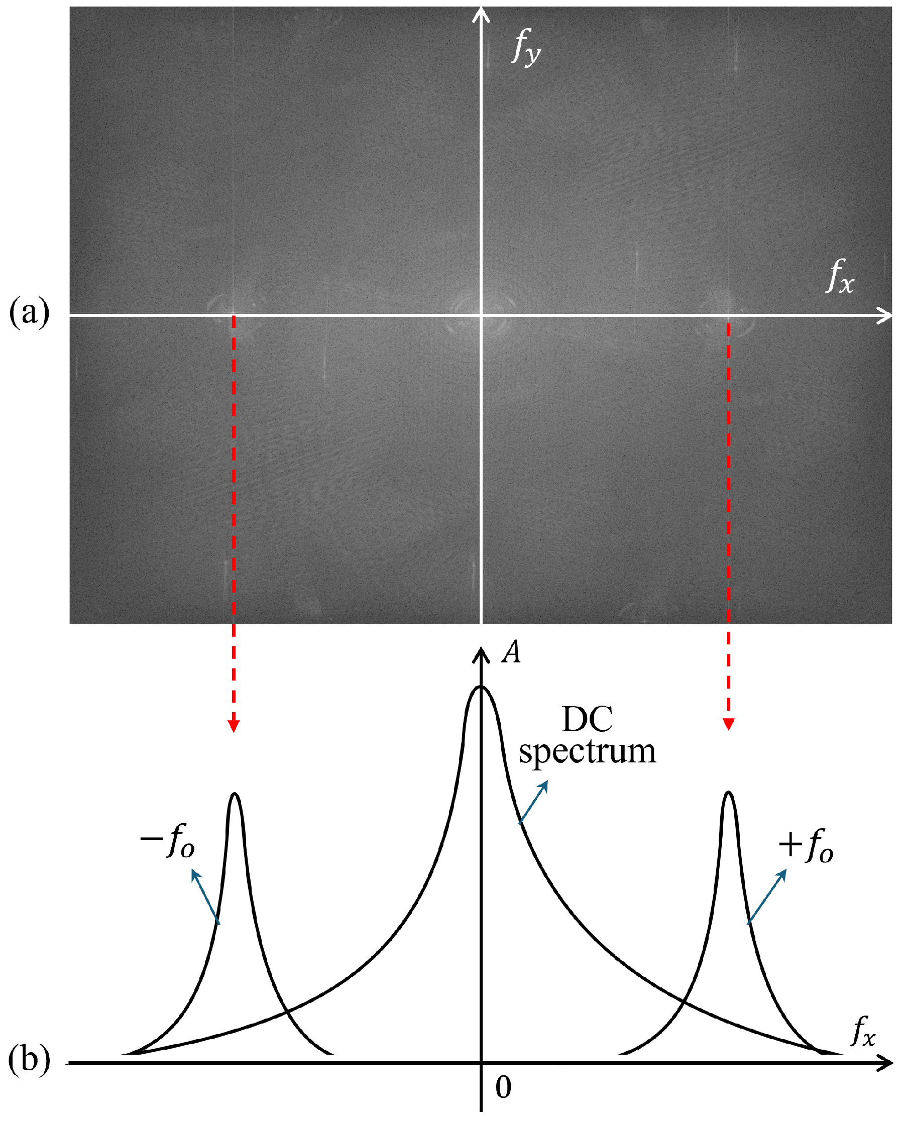
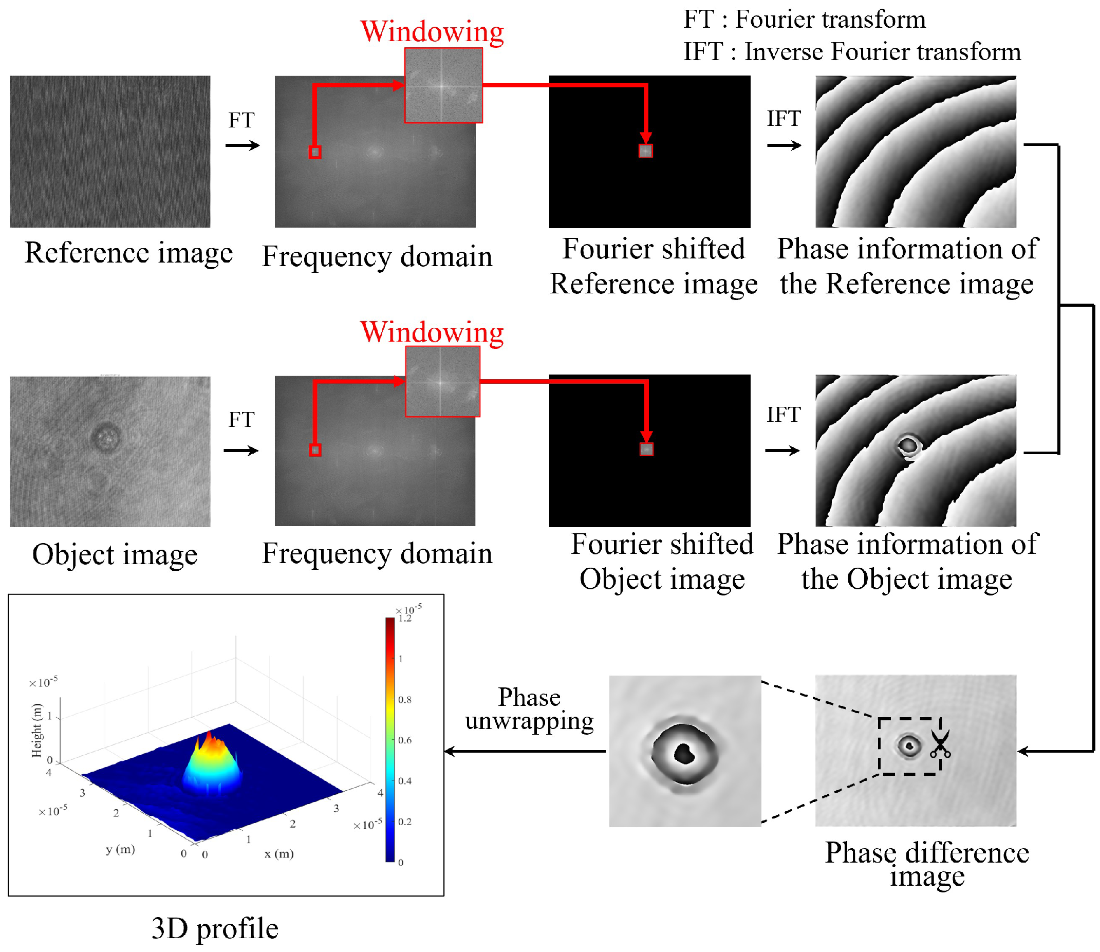
2.2. Image Processing for DHM

DHM uses the image processing methods to obtain the phase information and generate the 3D profiles of the object. The process diagram is illustrated in Figure 2. The object and reference images are Fourier transformed to obtain their respective frequency domains. To window the sideband from the frequency domain, the coordinates to be windowed are the same for both the frequency domains of the object and the reference images. This process can extract the phase information of the recorded hologram, but includes the DC term information. The WS is pasted in the center of the zero-matrix image. It is performed by the inverse Fourier transform to obtain the phase information contained in the object and reference images, respectively. By calculating the difference between each phase information, the phase scattered by the difference in the refractive indices between the surrounding medium and the object. The phase information in the image is converted into the height information using Equation (7) and displayed as the 3D profile. In this case, the DC term information included in the WS appears as the noise in the 3D profile. In DHM, where the phase information is extracted by image processing methods, it is difficult to exclude the DC term information when windowing the sideband. It is an issue that cannot be separated from the DHM system. To solve this problem, we describe the noise reduction method using the Kalman filter in Section 2.3.

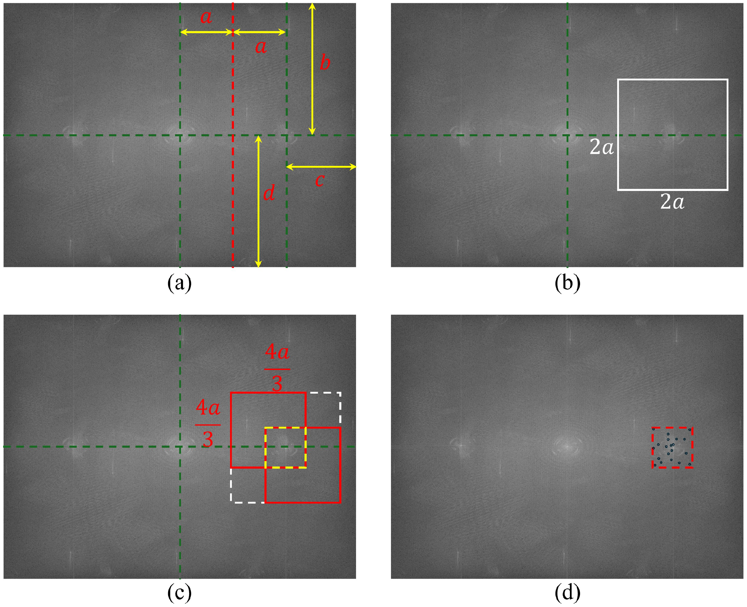
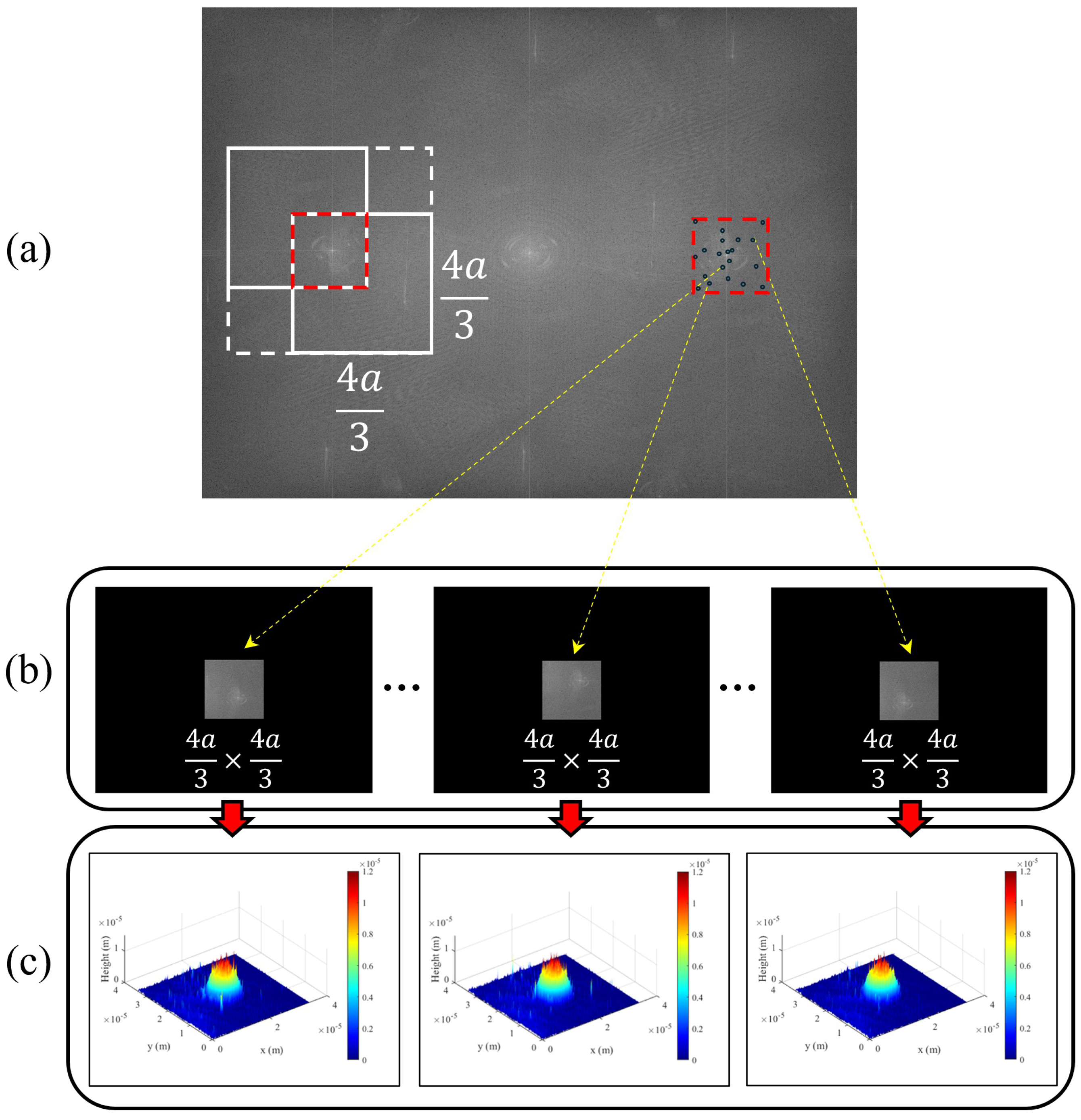
2.3. A Method for Determination of WS Size in DHM

Before describing the proposed method in this research, we explain the method to determine the maximum area of the sidebands to be windowed from the frequency domain. It determines the area of high-frequency information to be acquired. The maximum window area is a square with one side twice the half length of the distance from the DC term to the center of the sideband peak.
Figure 3 shows the method for determining the windowing area of the sideband [35]. In Figure 3a, a is half of the length from the DC term to the sideband peak. b is the distance from the peak of the sideband to the top of the image, and d is the distance from the bottom. c is the distance from the peak of the sideband to the edge of the image in the x-axis direction. We use the minimum of these parameters, and determine the maximum window area of the sideband as a square with sides twice the minimum. Figure 3b shows the maximum window area. It is the area of the high-frequency information that can be obtained. The proposed method in this research performs a windowing of 2/3 of this maximum area, as shown in Figure 3c. We choose several different coordinates, as shown in Figure 3d. We will explain the reason why we have to obtain the different coordinates in the next subsection. The maximum area of the information can be compensated for windowing it at the center with the determined windowing area.

2.4. A Method for Noise Reduction Using the Kalman Filter in DHM

This section describes the Kalman filter used in this research. The Kalman filter can be seen as a technique for estimating the true state of the system by correcting the uncertain data in the state-space model [36]. It is used for time-varying time series data, such as rocket trajectory estimation and navigation systems.
The Kalman filter is divided into two steps; a prediction step and an update step, which are repeated to estimate the true state. The prediction step predicts the state at the current time from the previous time’s state estimates. The prediction of the state in Kalman filter is calculated by Equations (8) and (9) [36],
x t + 1 α β = x t α β + v t α = 1 , 2 , 3 , , m β = 1 , 2 , 3 , , n
p t + 1 = p t + ω t
where x t α β indicates the state at the previous time, x t + 1 α β indicates the current state predicted from the state at the previous time, and v t indicates the observed noise. t is the time series. m and n are the width and the height of the image, respectively. In addition, p t and p t + 1 are the initial and predicted variances of the error covariance, and ω t is the process noise, respectively. The update step provides the correction of the predicted current state. The Kalman gain is used for correction; this is calculated using Equation (10) [36],
G = p t + 1 e p t + 1 e + v t ( e = 1 , 2 , , B )
x ^ t + 1 α β = x t + 1 α β + G × R t + 1 α β x t + 1 α β
where R t + 1 α β is the time series data, and is the observed current state. x ^ t + 1 α β corrected in this step is the new predicted pixel value. Finally, the error covariance used to calculate Kalman gain is corrected. This is calculated using Equation (12),
p t + 1 e + 1 = ( 1 G ) × p t + 1 e
where p t + 1 e + 1 is the variance corrected from predictions. These processes are performed for one time series. Kalman filter repeats it for each time series, repeatedly predicting and updating the state. The final output is the corrected current state x ^ t + 1 α β . In this research, the filtering target is stationary, and the aim is to remove noise. Therefore, the equation structure considers the observation noise and the process noise. As we mentioned earlier, we have to change time series to frequency series in this research.
A schematic diagram of the noise removal method using the Kalman filter is illustrated in Figure 4. The frequency domain of the recorded hologram is shown Figure 4a. Figure 4b shows several WSs from the frequency domain at random coordinates. They are pasted in the center of the zero-matrix image. Figure 4c shows the inverse Fourier transformed and the phase unwrapped image of Figure 4b. Therefore, Figure 4c shows the phase information of the object about each WS from the frequency domain at random coordinates. In this method, this is frequency series data. The order of the windowing is used as a frequency series to create data that is randomly noisy regardless of the frequency series. Kalman filter can remove the noise that appears regardless of frequency series. It can removes the noise caused by the DC term and enables the acquisition of even the high-frequency information on the object. As a result, Kalman filter can generate the detailed and the noise-reduced 3D profiles of the object in DHM.
By using Equation (7), the shape of the object using Kalman filter is calculated using Equation (13) [29],
H K i ( x , y ) = λ × Δ ϕ K i ( x , y ) 2 π × Δ r
In Equation (13), H K i ( x , y ) is the height information of the object after Kalman filtering. i is the number of frequency series data. Δ ϕ K i is the final value of p t + 1 e + 1 in Equation (12).

3. Experimental Setup and Results

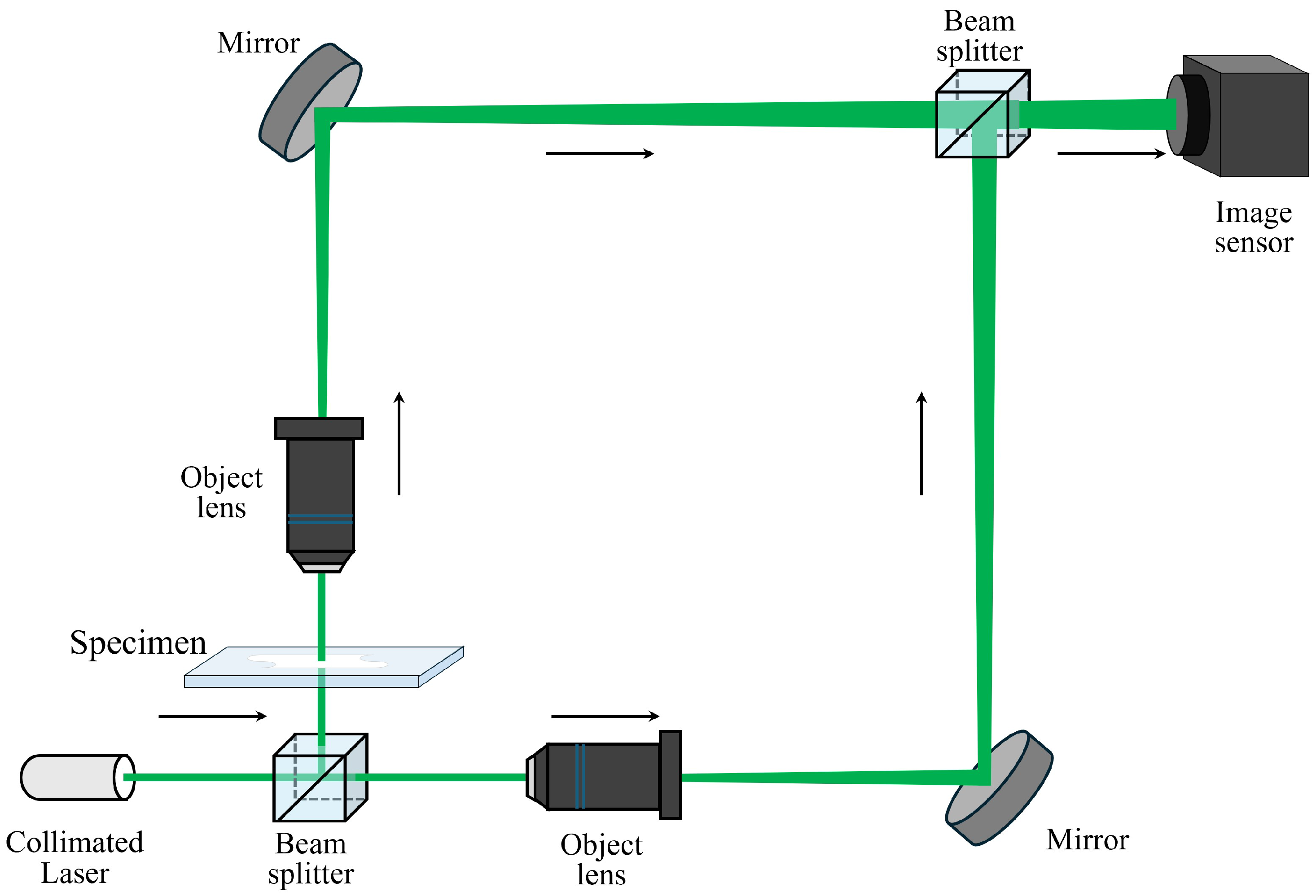
3.1. Experimental Setup

In this research, it is necessary to obtain an as wide as possible area of the phase information in the frequency domain. This means that the interference fringes in the hologram image have to be narrower. For this reason, the Mach–Zehnder interferometry is used in this research. Figure 5 illustrates the experimental setup. A 532 nm collimated laser (CPS532, Thorlabs, Newton, NJ, USA) is used as light source (4.5 mW output power). In addition, we use microspheres as the object to be observed. Microspheres are artificial spheres made of polystyrene with a diameter of 10 μm (02706-AB, SPI Supplies, West Chester, PA, USA). As they are artificial, their shape is defined, allowing for the calculation of noise reduction rates. The refractive index of the microsphere (polystyrene) is 1.59. Moreover, we use RBCs as the object, to measure the effect on objects of different sizes and shapes. The refractive indices of the RBCs and the surrounding medium are 1.42 and 1.34, respectively [12]. The magnification of two objective lenses (43-904, Edmund Optics, Barrington, NJ, USA) are both 40× (0.65 NA, 0.48 mm working distance). The generated holograms are recorded using a CMOS sensor (acA2500-14uc, Basler, Ahrensburg, Germany). The pixel size of the image sensor is 2.2 μm (H) × 2.2 μm (V), and the resolution is 2590 px (H) × 1942 px (V). The beam splitter in front of the image sensor was adjusted by tilting it and narrowing the interference fringes.

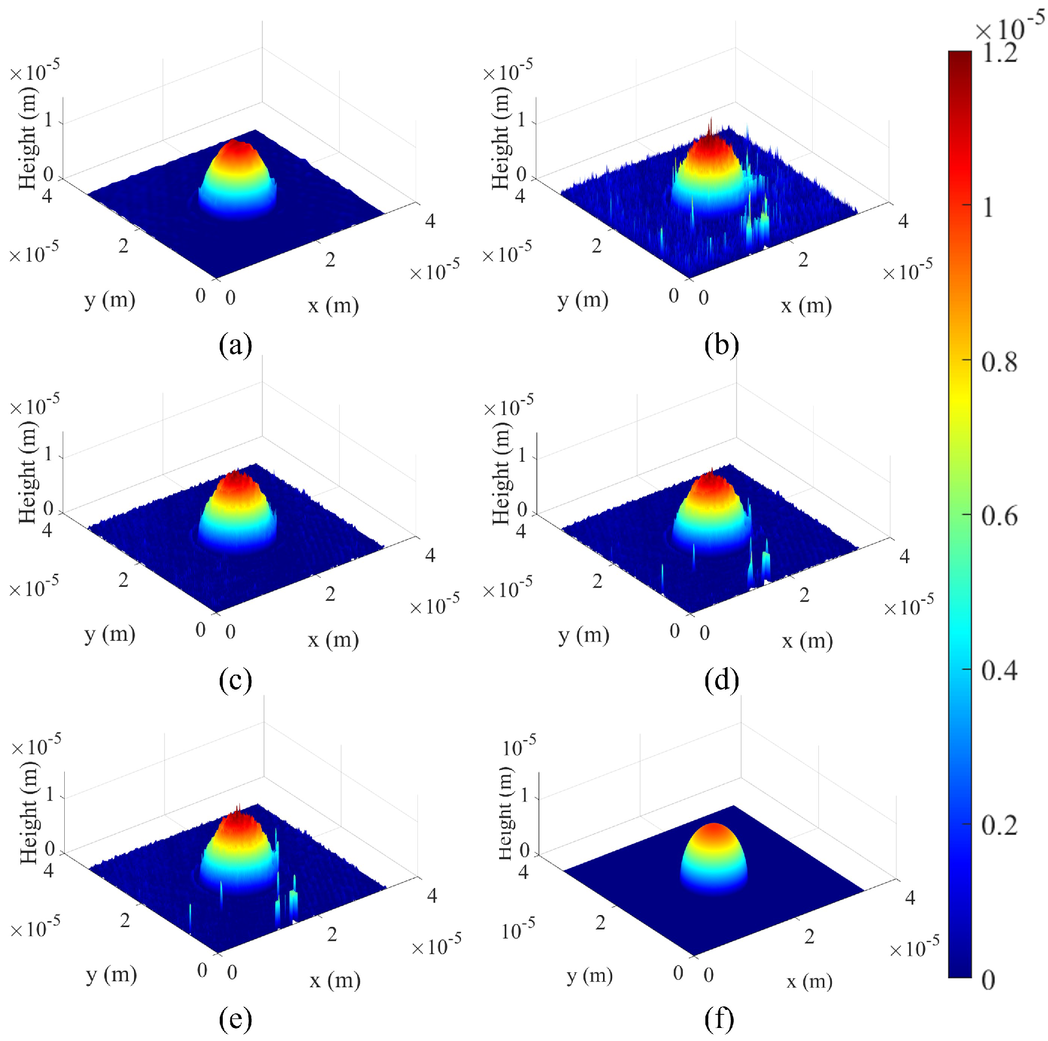
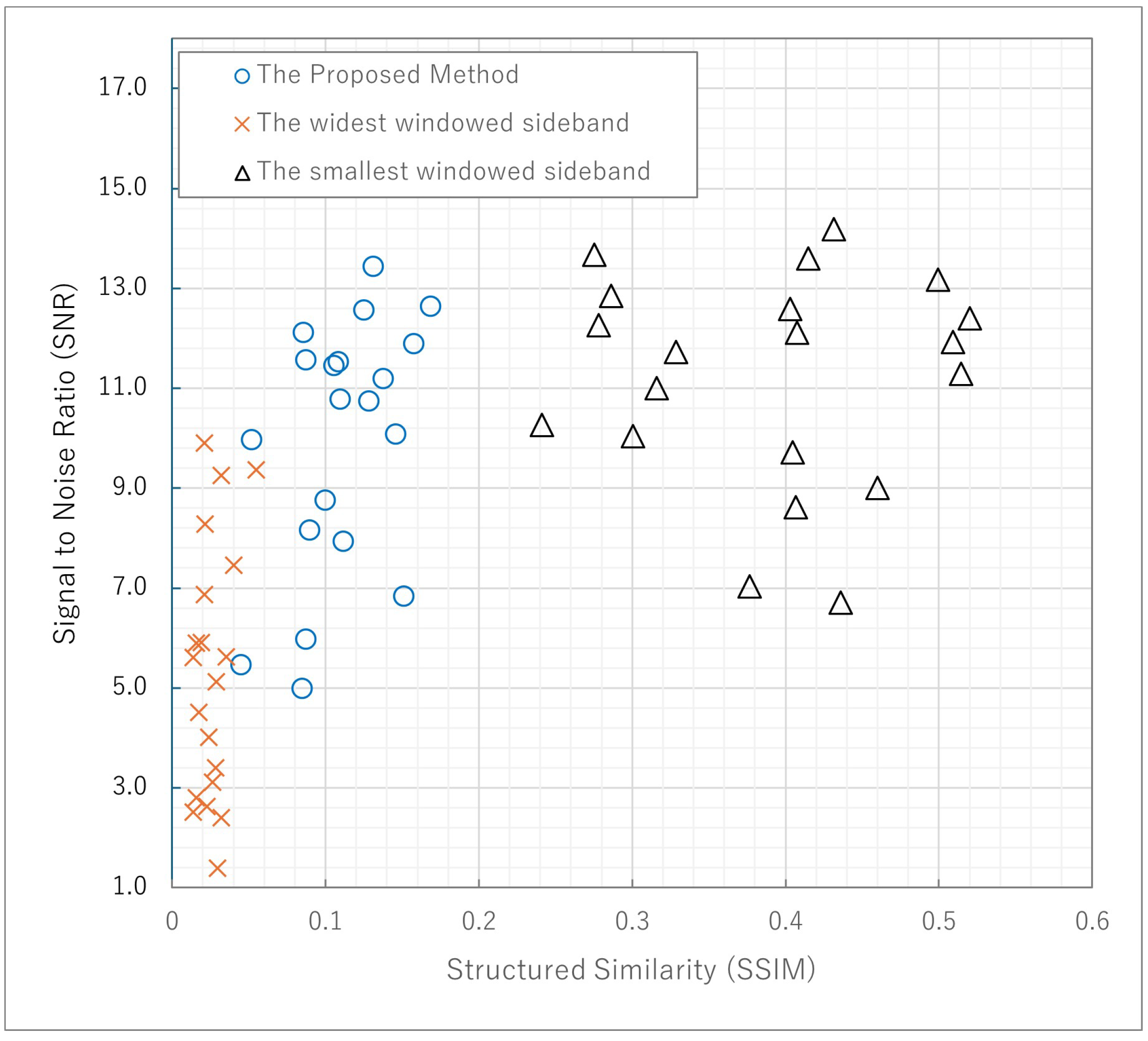
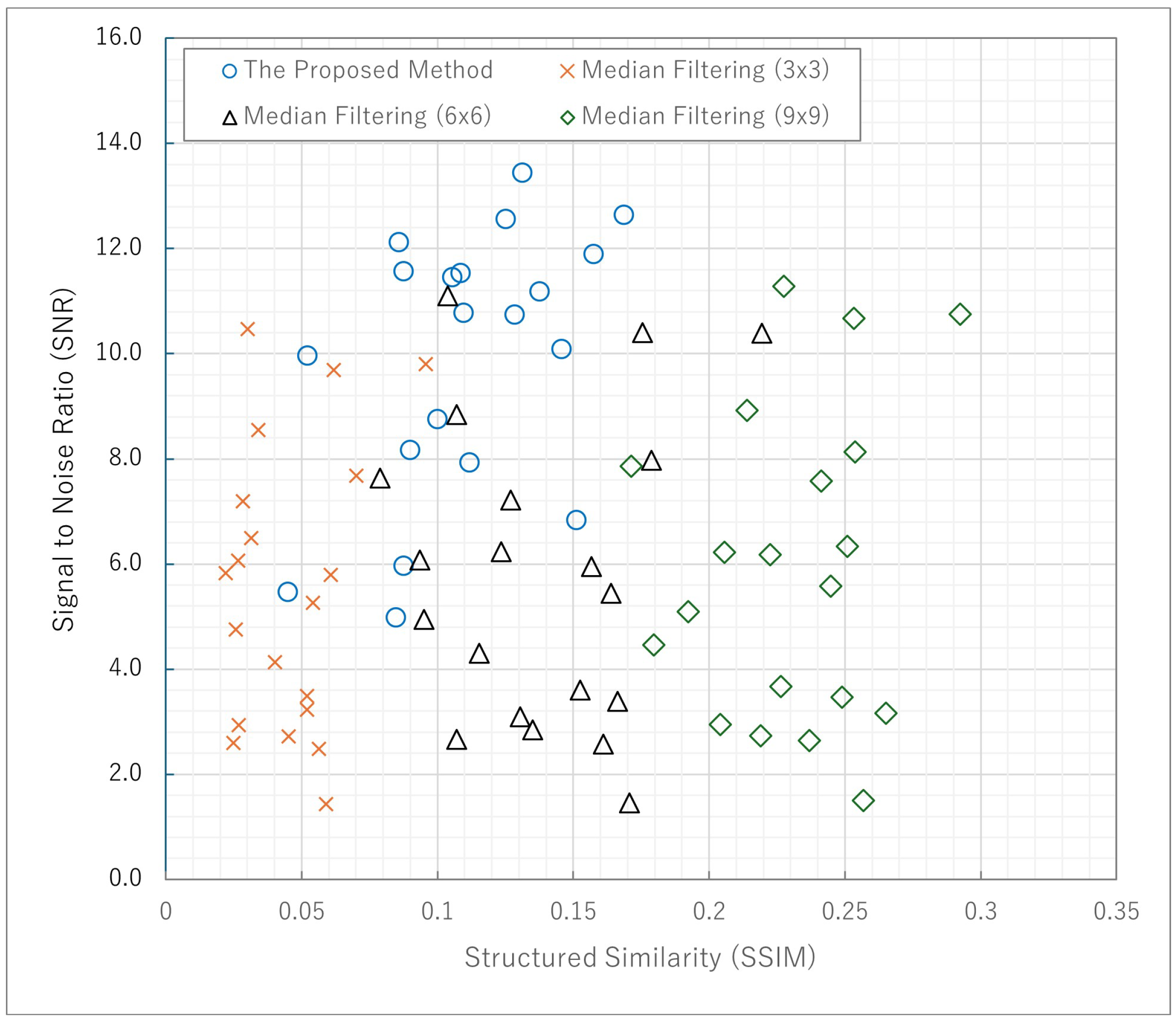
3.2. Experimental Result

Figure 6 shows the 3D profiles of the microsphere created by the proposed and the traditional methods. Here, the maximum windowing area is 782 px (H) × 782 px (V). The Goldstein phase-unwrapping algorithm [37] is used in this research to convert the wrapped phase into the continuous phase. When the phase region is reduced as shown in Figure 6a, the rough shape information of the object is obtained, and the noise is reduced. Widening the phase region, as shown in Figure 6b, can provide the detailed shape information of the object, but increase the noise. Therefore, the noise can be removed by our proposed method. In this research, 80 frequency series data points are prepared for the Kalman filter. The number of frequency series data points are set to a large number in order to increase the accuracy of the noise removal by the Kalman filter [36]. The area of the sideband cropping is fixed, and the coordinates of the windowing area of the sideband are selected at 80 locations. This process allows 80 frequency series data to be prepared from the single hologram image. The area to be cropped at this time is 521 px (H) × 521 px (V). Figure 6c shows the 3D profile with the noise removed by our proposed method. Figure 6d,e show the results of a Gaussian filter ( σ = 2 ) and a median filter (5 (H) × 5 (V)), respectively. The comparison of each 3D profile shows that our proposed method has the highest noise rejection. For the numerical comparison, the signal-to-noise ratio (SNR) [38] and the structured similarity index (SSIM) method [39] of each 3D profile are calculated. The ideal shape of the microsphere is used for the calculation as shown in Figure 6f. Table 1 compares the results of our proposed method with traditional methods and conventional filtering methods. Table 1 shows the highest SNR and SSIM values for Kalman filter. The results show that our proposed method is the best for removing the noise caused by the DC term of the DHM.
For the statistical analysis, 20 different microspheres are obtained randomly, and frequency series data and Kalman filters are obtained for each. The 3D Profile results obtained by the unfiltered method, Gaussian filtering, and median filtering are shown in Figure 7.
The blue bars in Figure 7a indicate the SNR values using our proposed method and the green bars represent the SNR values without filtering. The orange color dotted and solid horizontal lines show the variance of the SNR for the conventional method and our proposed method, respectively. In Figure 7b,c, the solid lines are the results of our proposed method, and the dotted lines are the results of the respective conventional methods, where blue lines show the average SNR values and orange lines show their variance. In the unfiltered method, it can be seen that there is more noise, and the SNR values are smaller than our proposed method. As shown in Figure 7, the Kalman filter reduces the noise and improves the SNR values for all objects. When acquiring the high-frequency information on the object, the noise due to the DC term is generated due to the larger sideband windowing area. Therefore, the unfiltered 3D Profile is noisy and has a low SNR value. It can be seen that the Kalman filter reduces the noise generated by the DC term, and allows for a more accurate shape to be obtained. Figure 7b shows that Gaussian filtering improves the SNR with increasing the sigma values. It can also be seen from Figure 7c that increasing the filtering area for median filter improves the SNR. However, these operations result in the smoothing of the obtained 3D information, which also results in the loss of the high-frequency information on the object. The Kalman filter can accommodate it, and does not smooth out the high-frequency information. In addition, the variances of Gaussian and median filtering are considerably larger compared to our proposed method. The value of the variance is related to the stability of the filtering, suggesting that random noise is likely to remain. To test it, the correlation between SNR and SSIM was used in this research.
The correlation between SNR and SSIM for different microspheres generated by the same method are shown in Figure 8. The vertical axis shows the SNR value and the horizontal axis shows the SSIM value. Figure 8 shows that our proposed method retains the high spatial frequency information of the object and shows the high SNR and SSIM values.
As shown in Figure 9, SNR and SSIM are improved as the filtering area of the median filtering increases. However, when the filtering area of the median filtering is increased, that much higher spatial frequency information of the object is smoothed out.
Figure 10 shows that increasing the sigma value of the Gaussian filter improves SNR and SSIM. However, increasing the sigma value of the Gaussian filter suppresses the high spatial frequency information of the object. Our proposed method shows the high values with respect to SNR and SSIM while containing the high spatial frequency information.
In Figure 9 and Figure 10, we can verify the filtering effect, but these filtering methods are not exactly comparable because they smooth out the high spatial frequency information of the objects. However, our proposed method shows comparable or better results than them while including the high spatial frequency information.
In this research, Kalman filter uses random sideband windowing coordinates. Therefore, the result after filtering changes depending on the order of the acquired coordinates and frequency series data. Figure 11 shows the SNR values and variances for each of 20 Kalman filter runs on the same object. The dotted line in Figure 11 shows the results of our proposed method, and the solid line shows the results of the unfiltered method. The results of our proposed method show high values for all SNRs, indicating that noise removal is possible while retaining high frequency information. In addition, our proposed method has very small variance. The results show that random elements in the generation of frequency series data do not significantly affect the results and performance.
The 3D profile of the sample number 1 in Figure 7 is shown in Figure 12. Figure 12a,b are the 3D profile with the unfiltered and our proposed methods, respectively. In Figure 12a, the shape of the object may not be reconstructed and the object is squashed. This shape is due to the high noise in the image and the phase unwrapping does not work well. Kalman filter generates the 3D profile from sidebands selected at multiple coordinates, which is frequency series data. Therefore, it can compensate for missing information and reconstruct the shape of the object, as shown in Figure 12b.
The results of the RBCs are shown in Figure 13. The area where the sidebands are windowed is 676 px (H) × 676 px (V). Figure 13a,c,e are the unfiltered 3D profiles and Figure 13b,d,f are the 3D profiles after respective Kalman filter. In the unfiltered 3D profile, we can recognize the high frequency noise on both the background and the RBCs randomly. After Kalman filter, the 3D profile has reduced the noise and the detailed shape of the 3D profile can be obtained. These results show that our proposed method is effective in removing noise even for objects that are not uniform in shape and size.

4. Conclusions

In this research, the noise filtering method, which is not available in conventional methods, has been proposed to reduce the noise due to the DC term in DHM. To confirm the effectiveness, a comparison has been made with the traditional filtering methods. Our proposed method has shown the advantage of higher noise reduction than other filtering methods and the detailed 3D profiles contain high spatial frequencies with stability. Filtering methods with the single masking window result in lower spatial frequencies for the 3D profile of the object. In addition, when attempting to acquire higher spatial frequency information, the increased and accurately detailed information on objects may not be obtained. This is a trade-off, and has been a problem. Our method proposed in this research has solved this trade-off by acquiring high spatial frequency information and removing the noise generated in the image processing. Another advantage is that when the 3D profile of the object may not be reconstructed in the single masking window, multiple frequency series data can be used to reconstruct the shape of the object. In this research, an arbitrary amount of data were used for the frequency series data; when the amount of data increases, the accuracy of the likelihood is enhanced, but the processing time increases, which is a trade-off. Therefore, the user needs to choose the appropriate value depending on the object and the experimental environment.

Author Contributions

Conceptualization, T.O. and H.-W.K.; data curation, T.O.; writing—original draft preparation, T.O.; writing—review and editing, M.C. and M.-C.L.; supervision, M.-C.L. All authors have read and agreed to the published version of the manuscript.

Funding

This research received no external funding.

Data Availability Statement

All data underlying the results are available as part of the article and no additional source data are required.

Conflicts of Interest

The authors declare no conflicts of interest.

Abbreviations

The following abbreviations are used in this manuscript:
2DTwo-dimensional
3DThree-dimensional
DCDirect current
DHMDigital holographic microscopy
RBCRed blood cell
SNRSignal-to-noise ratio
SSIMStructured similarity
WSWindowed sideband

References

  1. Nguyen, T.M.; Kim, N.; Kim, D.H.; Le, H.L.; Piran, M.J.; Um, S.J.; Kim, J.H. Deep learning for human disease detection, subtype classification, and treatment response prediction using epigenomic data. Biomedicines 2021, 9, 1733. [Google Scholar] [CrossRef] [PubMed]
  2. Mishra, S.; Dash, A.; Jena, L. Use of deep learning for disease detection and diagnosis. In Bio-Inspired Neurocomputing; Springer: New York, NY, USA, 2021; pp. 181–201. [Google Scholar]
  3. Yousaf, F.; Iqbal, S.; Fatima, N.; Kousar, T.; Rahim, M.S.M. Multi-class disease detection using deep learning and human brain medical imaging. Biomed. Signal Process. Control 2023, 85, 104875. [Google Scholar] [CrossRef]
  4. Tchagna Kouanou, A.; Mih Attia, T.; Feudjio, C.; Djeumo, A.F.; Ngo Mouelas, A.; Nzogang, M.P.; Tchito Tchapga, C.; Tchiotsop, D. An overview of supervised machine learning methods and data analysis for COVID-19 detection. J. Healthc. Eng. 2021, 2021, 4733167. [Google Scholar] [CrossRef]
  5. Zoabi, Y.; Deri-Rozov, S.; Shomron, N. Machine learning-based prediction of COVID-19 diagnosis based on symptoms. NPJ Digit. Med. 2021, 4, 1–5. [Google Scholar] [CrossRef]
  6. Rehman, A.; Iqbal, M.A.; Xing, H.; Ahmed, I. COVID-19 detection empowered with machine learning and deep learningtechniques: A systematic review. Appl. Sci. 2021, 11, 3414. [Google Scholar] [CrossRef]
  7. Subramanian, N.; Elharrouss, O.; Al-Maadeed, S.; Chowdhury, M. A review of deep learning-based detec-tion methods for COVID-19. Comput. Biol. Med. 2022, 143, 105233. [Google Scholar] [CrossRef]
  8. O’Connor, T.; Shen, J.B.; Liang, B.T.; Javidi, B. Digital holographic deep learning of red blood cells for field-portable, rapid COVID-19 screening. Opt. Lett. 2021, 46, 2344–2347. [Google Scholar] [CrossRef]
  9. O’Connor, T.; Santaniello, S.; Javidi, B. COVID-19 detection from red blood cells using highly comparative time-series analysis (HCTSA) in digital holographic microscopy. Opt. Express 2022, 30, 1723–1736. [Google Scholar] [CrossRef]
  10. O’Connor, T.; Javidi, B. COVID-19 screening with digital holographic microscopy using intra-patient probability functions of spatio-temporal bio-optical attributes. Opt. Express 2022, 13, 5377–5389. [Google Scholar] [CrossRef]
  11. El-Schich, Z.; Leida Mölder, A.; Gjörloff Wingren, A. Quantitative phase imaging for label-free analysis of cancer cells—Focus on digital holographic microscopy. Appl. Sci. 2018, 8, 1027. [Google Scholar] [CrossRef]
  12. Anand, A.; Chhaniwal, V.K.; Patel, N.R.; Javidi, B. Automatic identification of malaria-infected RBC with digital holographic microscopy using correlation algorithms. IEEE Photonics J. 2012, 4, 1456–1464. [Google Scholar] [CrossRef]
  13. Javidi, B.; Markman, A.; Rawat, S.; O’Connor, T.; Anand, A.; Andemariam, B. Sickle cell disease diagnosis based on spatiotemporalcell dynamics analysis using 3D printed shearing digital holographic microscopy. Opt. Express 2018, 26, 13614–13627. [Google Scholar] [CrossRef]
  14. Gabor, D. A new microscopic principle. Nature 1948, 161, 777–778. [Google Scholar] [CrossRef]
  15. Goodman, J.W. Digital image formation from electronically detected holograms. In Proceedings of the SPIE 0010, Computerized Imaging Techniques, Washington, DC, USA, 1 July 1967. [Google Scholar]
  16. Kim, Y.; Park, S.; Baek, H.; Min, S.W. Voxel characteristic estimation of integral imaging display system using self-interference incoherent digital holography. Opt. Express 2022, 30, 902–913. [Google Scholar] [CrossRef]
  17. Ahar, A.; Birnbaum, T.; Chlipala, M.; Zaperty, W.; Mahmoudpour, S.; Kozacki, T.; Kujawinska, M.; Schelkens, P. Comprehensive performance analysis of objective quality metrics for digital holography. Signal Process. Image Commun. 2021, 97, 116361. [Google Scholar] [CrossRef]
  18. Shevkunov, I.; Katkovnik, V.; Claus, D.; Pedrini, G.; Petrov, N.V.; Egiazarian, K. Spectral object recognition in hyperspectral holography with complex-domain denoising. Sensors 2019, 19, 5188. [Google Scholar] [CrossRef] [PubMed]
  19. Bordbar, B.; Zhou, H.; Banerjee, P.P. 3D object recognition through processing of 2D holograms. Appl. Opt. 2019, 58, G197–G203. [Google Scholar] [CrossRef]
  20. Lokesh Reddy, B.; Nelleri, A. Single-Pixel Compressive Digital Holographic Encryption System Based on Circular Harmonic Key and Parallel Phase Shifting Digital Holography. Int. J. Opt. 2022, 2022, 6298010. [Google Scholar] [CrossRef]
  21. Girija, R.; Singh, H.; Abirami, G. Optical medical image encryption based on digital hologram in various domains. J. Opt. 2024, 53, 458–467. [Google Scholar] [CrossRef]
  22. Reddy, B.L.; Ramachandran, P.; Nelleri, A. Optimal Fresnelet sparsification for compressive complex wave retrieval from an off-axis digital Fresnel hologram. Opt. Eng. 2021, 60, 073102. [Google Scholar] [CrossRef]
  23. Yoshikawa, N.; Miyake, T. Omnidirectional 3D shape measurement using image outlines reconstructed from gabor digital holography. Opt. Commun. 2023, 529, 129080. [Google Scholar] [CrossRef]
  24. Butola, A.; Kanade, S.R.; Bhatt, S.; Dubey, V.K.; Kumar, A.; Ahmad, A.; Prasad, D.K.; Senthilkumaran, P.; Ahluwalia, B.S.; Mehta, D.S. High space-bandwidth in quantitative phase imaging using partially spatially coherent digital holographic microscopy and a deep neural network. Opt. Express 2020, 28, 36229–36244. [Google Scholar] [CrossRef] [PubMed]
  25. Kim, H.W.; Lee, J.; Anand, A.; Cho, M.; Lee, M.C. Phase Differences Averaging (PDA) Method for Reducing the Phase Error in Digital Holographic Microscopy (DHM). J. Korea Inst. Inf. Commun. Eng. 2023, 21, 90–97. [Google Scholar] [CrossRef]
  26. Javidi, B.; Carnicer, A.; Anand, A.; Barbastathis, G.; Chen, W.; Ferraro, P.; Goodman, J.W.; Horisaki, R.; Khare, K.; Kujawinska, M.; et al. Roadmap on digital holography. Opt. Express 2023, 29, 35078–35118. [Google Scholar] [CrossRef] [PubMed]
  27. Kim, H.W.; Cho, M.; Lee, M.C. Noise reduction method using a variance map of the phase differences in digital holographic microscopy. ETRI J. 2022, 45, 131–137. [Google Scholar] [CrossRef]
  28. Kim, H.W.; Cho, M.; Lee, M.C. Noise Filtering Method of Digital Holographic Microscopy for Obtaining an Accurate Three-Dimensional Profile of Object Using aWindowed Sideband Array (WiSA). Sensors 2022, 22, 4844. [Google Scholar] [CrossRef] [PubMed]
  29. Shin, S.; Yu, Y. Fine metal mask 3-dimensional measurement by using scanning digital holographic microscope. J. Korean Phys. Soc 2018, 72, 863–867. [Google Scholar] [CrossRef]
  30. Li, J.; Li, B.; Zhang, X. Digital holographic microscopy measures underwater microorganism. In Proceedings of the SPIE 11427, Second Target Recognition and Artificial Intelligence Summit Forum, Changchun, China, 31 January 2020. [Google Scholar]
  31. Kim, H.W.; Cho, M.; Lee, M.C. Image Processing Techniques for Improving Quality of 3D Profile in Digital Holographic Microscopy Using Deep Learning Algorithm. Sensors 2024, 24, 1950. [Google Scholar] [CrossRef]
  32. Kalman, R.E. A new approach to linear filtering and prediction problems. J. Fluids Eng. 1960, 82, 35–45. [Google Scholar] [CrossRef]
  33. Tang, H.; Tang, Y.; Su, Y.; Feng, W.; Wang, B.; Chen, P.; Zuo, D. Feature extraction of multi-sensors for early bearing fault diagnosis using deep learning based on minimum unscented kalman filter. Eng. Appl. Artif. Intell. 2024, 127, 107138. [Google Scholar] [CrossRef]
  34. Park, G. Optimal vehicle position estimation using adaptive unscented Kalman filter based on sensor fusion. Mechatronics 2024, 99, 103144. [Google Scholar] [CrossRef]
  35. Kim, H.W.; Cho, M.; Lee, M.C. A Novel Image Processing Method for Obtaining an Accurate Three-Dimensional Profile of Red Blood Cells in Digital Holographic Microscopy. Biomimetics 2023, 8, 563. [Google Scholar] [CrossRef] [PubMed]
  36. Kim, H.W.; Cho, M.; Lee, M.C. Three-Di-mensional (3D) Visualization under Extremely Low Light Conditions Using Kalman Filter. Sensors 2023, 23, 7571. [Google Scholar] [CrossRef]
  37. Goldstein, R.M.; Zebker, H.A.; Werner, C.L. Satellite radar interferometry: Two-dimensional phase unwrapping. Radio Sci. 1988, 23, 713–720. [Google Scholar] [CrossRef]
  38. Gonzalez, R.C.; Woods, R.E. Digital Image Processing, 4th ed.; Pearson: New York, NY, USA, 2018. [Google Scholar]
  39. Wang, Z.; Bovik, A.C.; Sheikh, H.R.; Simoncelli, E.P. Image quality assessment: From error visibility to structural similarity. IEEE Trans. Image Process 2004, 13, 600–612. [Google Scholar] [CrossRef] [PubMed]
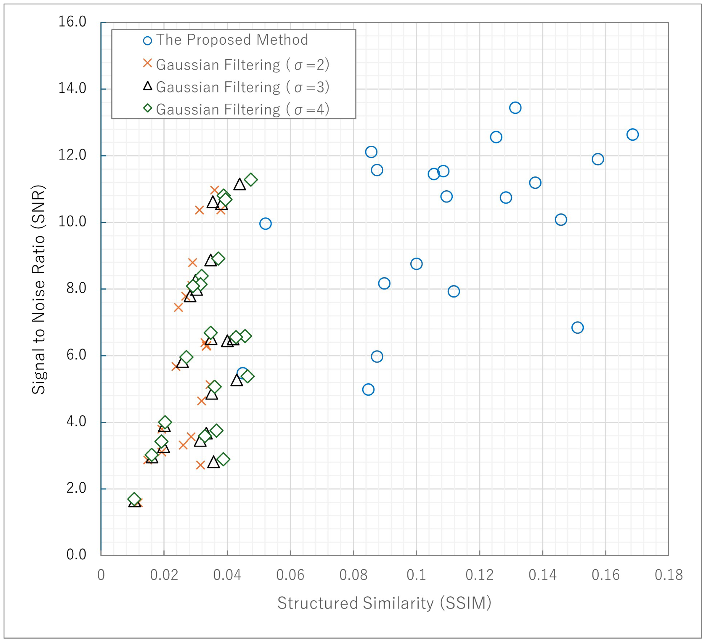
Figure 1. Fourier transform result of the recorded hologram. (a) 2D and (b) 1D (cross-section).
Electronics 14 00338 g001
Figure 2. Image processing to create a 3D profile in DHM.
Electronics 14 00338 g002
Figure 3. Multi-coordinate sideband windowing method. (a) Determination of the WS size. (b) Range of high-frequency information to be obtained. (c) Range of multiple coordinate selections. (d) Result of a random selection of several coordinates.
Electronics 14 00338 g003
Figure 4. Schematic diagram of Kalman filtering in DHM. (a) Multiple selections of WS and windowing coordinates. (b) WSs at random coordinates. (c) Images with each phase information of sideband (frequency series data).
Electronics 14 00338 g004
Figure 5. Schematic diagram of the experimental setup.
Electronics 14 00338 g005
Figure 6. Three-dimensional profiles of microsphere for (a) the smallest WS and (b) the widest WS. The result of (c) Kalman filter, (d) Gaussian filtering and (e) median filtering. (f) The ideal shape of microsphere.
Electronics 14 00338 g006
Figure 7. Comparison result of the Kalman filtering with (a) the unfiltered method, (b) Gaussian filtering, and (c) median filtering.
Electronics 14 00338 g007
Figure 8. Comparison between Kalman filtering and the unfiltered methods using a correlation between SNR and SSIM.
Electronics 14 00338 g008
Figure 9. Comparison between Kalman filtering and median filtering using a correlation between SNR and SSIM.
Electronics 14 00338 g009
Figure 10. Comparison between Kalman filtering and Gaussian filtering using a correlation between SNR and SSIM.
Electronics 14 00338 g010
Figure 11. Variance of randomness of noise reduction by Kalman filter.
Electronics 14 00338 g011
Figure 12. Effect of Kalman filter on noise reduction. (a) The 3D profile where the shape may not be reconstructed due to high noise. (b) Kalman filtering results.
Electronics 14 00338 g012
Figure 13. 3D profiles of RBCs. (a,c,e) The unfiltered method. (b,d,f) The Kalman filtering method.
Electronics 14 00338 g013
Table 1. Comparison of different filtering methods using SNR and SSIM.
SNR (dB)SSIM
Unfiltered9.9070.02100
Kalman filter11.570.08751
Gaussian filter10.970.03598
Median filter10.910.06733
Disclaimer/Publisher’s Note: The statements, opinions and data contained in all publications are solely those of the individual author(s) and contributor(s) and not of MDPI and/or the editor(s). MDPI and/or the editor(s) disclaim responsibility for any injury to people or property resulting from any ideas, methods, instructions or products referred to in the content.

