Ultra-Short-Term Photovoltaic Power Prediction Based on BiLSTM with Wavelet Decomposition and Dual Attention Mechanism

Abstract

Photovoltaic power generation relies on sunlight conditions, and traditional prediction models find it difficult to capture the deep features of power data, resulting in low prediction accuracy. In addition, there are problems such as outliers and missing values in the data collected on site. This article proposes an ultra-short-term photovoltaic power generation prediction model based on wavelet decomposition, a dual attention mechanism, and a bidirectional long short-term memory network (W-DA-BiLSTM), aiming to address the limitations of existing deep learning models in processing nonlinear data and automatic feature extraction and optimize for the common problems of outliers and missing values in on-site data collection. This model uses the quartile range method for outlier detection and multiple interpolation methods for missing value completion. In the prediction section, wavelet decomposition is used to effectively handle the volatility and nonlinear characteristics of photovoltaic power generation data, while the bidirectional long short-term memory network (LSTM) structure and dual attention mechanism enhance the model’s comprehensive learning ability for time series data. The experimental results show that compared with the SOTA method, the model proposed in this paper has higher accuracy and efficiency in predicting photovoltaic power generation and can effectively address common random fluctuations and nonlinear problems in photovoltaic power generation.

1. Introduction

With the continuous growth of global electricity demand and the increasing demand for environmental protection, the traditional energy structure is under pressure to optimize and improve [1]. In this context, the proportion of renewable energy, especially photovoltaic power generation, continues to increase in the global energy structure. At the end of August 2024, the installed capacity of solar power generation was about 750 million kilowatts, a year-on-year increase of 48.8% [2]. However, the randomness and volatility of photovoltaic power generation pose new challenges to the operational stability and scheduling strategies of the power system [3]. Especially in situations where large-scale electrical energy storage is difficult and there is insufficient coordination in source network planning, the stability of the power system will be affected [4]. Therefore, accurate prediction of photovoltaic power generation has become a key technical requirement to maintain the balance between supply and demand of the power grid and ensure safe operation of the system [5], which is of profound importance for sustainable development and optimized operation of the power system.

For the prediction of photovoltaic power generation, scholars have proposed various prediction methods [6]. According to the predicted time scale, they are divided into several different categories: ultra-short-term, short-term, and medium/long-term. According to the classification of prediction methods, they can be divided into conventional methods, including physical models and traditional statistical models, and methods based on artificial intelligence algorithms, including machine learning methods and deep learning methods [7].

Physical models are based on the principles and mathematical formulas of photovoltaic power generation. They construct mathematical models using data obtained from numerical weather prediction, including solar radiation, temperature, humidity, cloud cover, air pressure, and wind speed, without requiring historical data. Mayer et al. [8] investigated various physical PV power prediction models based on numerical weather prediction data, ranging from simple radiation conversion formulas to complex three-dimensional energy balance models. They compared the performance of these models and found that the complexity of the models is not entirely positively correlated with prediction accuracy. Moreover, the performance of the models is significantly influenced by weather conditions and data quality. Lorenz et al. [9] further developed a physical model for hourly PV power forecasting for the next day based on site-specific irradiance forecasts provided by European Centre for Medium-Range Weather Forecasts. This model employed a time-segmented optimization method to enhance the reliability of short-term predictions. However, the accuracy of these studies’ predictions heavily depends on the precision of numerical weather prediction information. Current NWP methods are constrained by hardware costs and technical complexity, making it difficult to meet the demands of extreme weather conditions [10]. Additionally, complex physical models face limitations in computational efficiency and broad applicability, particularly in capturing the nonlinear impacts of extreme weather on photovoltaic power.

Traditional statistical models use pure mathematical equations to process historical data such as solar radiation and photovoltaic power generation and make predictions through curve fitting, parameter estimation, and correlation analysis. Common methods include regression models [11], Kalman filters [12], and Markov chains [13]. Hanmin Sheng et al. [11] proposed a Gaussian weighted regression method based on density local outlier factors to predict short-term photovoltaic power generation. Jin Dong et al. [14] analyzed the probabilistic behavior of solar energy and proposed a novel stochastic photovoltaic power prediction model based on a stochastic state space model and Kalman filter. FO Hocaoglu et al. [15] developed a statistical method based on a novel Markov process to predict solar irradiance. Statistical models simplify the process of model establishment and have high robustness. However, they perform poorly in the face of new environments with statistical characteristics different from the training data and require a large amount of numerical calculations during the prediction process, making it difficult to meet the prediction speed requirements for ultra-short-term photovoltaic power generation prediction [16].

Machine learning, also known as generalized statistical models, can effectively extract high-dimensional complex nonlinear features and directly map them to the output with fast prediction speed. Therefore, machine learning-based prediction methods have been widely applied in the problem of predicting time series [17]. The commonly used machine learning algorithms for ultra-short-term photovoltaic power prediction include artificial neural networks (ANNs), support vector machines (SVMs), extreme learning machines (ELMs), and random forests (RFs). Ghimire et al. [18] developed an improved ANN model to enhance the predictive ability of photovoltaic power. William et al. [19] considered random weather conditions and proposed a hybrid model based on a genetic algorithm and SVM for short-term prediction of photovoltaic power generation. Behera M K et al. [20] proposed a new prediction structure based on particle swarm optimization (PSO) and ELM, using PSO to optimize the weight parameters of the ELM to achieve real-time prediction of photovoltaic power. Pan et al. [21] developed a photovoltaic prediction method based on cluster analysis, random forest, and ensemble techniques, which divides weather conditions into different systems through random forest.

With the increase in historical data, the ability of machine learning is limited in the presence of many input variables, which can easily lead to over-fitting. Deep learning has higher feature extraction capabilities than machine learning and can significantly improve the over-fitting problem in machine learning. Therefore, some scholars have begun to focus on using deep learning methods for ultra-short-term photovoltaic power generation prediction, in which LSTM or bidirectional LSTM (BiLSTM) is used to extract the intrinsic features of historical data and their corresponding meteorological data, achieving good experimental results. Wang et al. [22] proposed a hybrid deep learning model that combines LSTM and a Convolutional Neural Network (CNN), where the temporal features of the data are extracted by LSTM and the spatial features are extracted by a CNN. The results indicate that the proposed LSTM-CNN model has high prediction accuracy. Zhen et al. [23] proposed a hybrid model combining BiLSTM and a genetic algorithm to improve prediction accuracy. Abdel Basset et al. [24] introduced a data-driven PV Net to predict short-term photovoltaic power and redesigned the gates of a Gated Recurrent Network (GRU) using convolutional layers. The results indicate that PV Net improves the feature extraction of photovoltaic power time series and has high accuracy. Shi Peiming et al. [25] proposed a hybrid forecasting method combining Temporal Convolutional Networks (TCNs), bidirectional long short-term memory networks (BiLSTM), and Echo State Networks (ESNs). The method employs Complete Ensemble Empirical Mode Decomposition with Adaptive Noise to decompose power data into a series of relatively stationary sub-power sequences with distinct fluctuation patterns. These reconstructed power sequences, along with other feature sequences, are then fed into the TCN-BiLSTM–Attention–ESN hybrid model for forecasting. Huang Li et al. [26] introduced an ultra-short-term photovoltaic power forecasting approach based on the Transformer encoder. This method reconstructs the input matrix using historical meteorological data and numerical weather prediction data. Multilayer perceptrons are used to generate input embeddings, and the multi-head self-attention mechanism is employed to automatically explore the intrinsic coupling relationships among data features.Huang Ze et al. [27] developed an ultra-short-term photovoltaic power forecasting method based on similar-day clustering, swarm decomposition, and a deep learning model combining MBI-PBI-ResNet. This method enhances forecasting accuracy by extracting temporal features influenced by multi-variable weather conditions, while simultaneously capturing local waveform spatial features of multi-scale components and long-term dependencies in the time series.

The above studies demonstrate that effective combinations of neural networks can improve the accuracy of nonlinear time series forecasting. However, these methods fail to account for the specific characteristics of actual photovoltaic data in their design. Moreover, the vast majority of the literature has not paid attention to the handling of outliers. Due to various interferences that may occur during on-site data collection, such as data loss caused by communication failures, the quality of collected historical photovoltaic power data may vary. Outliers increase the difficulty of analysis work and may introduce analysis errors, affecting prediction efficiency. Therefore, this article proposes an innovative ultra-short-term photovoltaic power generation prediction model, which uses interquartile range (IQR) for outlier detection and multiple interpolation (MI) for missing value completion to achieve data preprocessing. The prediction part is a bidirectional long short-term memory network (W-DA-BiLSTM) enhanced by combining wavelet decomposition and a dual attention mechanism. Wavelet decomposition can effectively consider the volatility, nonlinear characteristics, and temporal dependence of photovoltaic power generation data, providing more refined inputs for deep learning models. The bidirectional LSTM structure enables the model to simultaneously learn the forward and backward features of time series data, thereby comprehensively capturing the dynamic changes in time series. The introduced dual attention mechanism not only focuses on key time points in time series data but also weights the internal features of the model, enhancing its ability to learn important information.

The contributions of this article are as follows:

• By using the quartile range method for outlier detection and the multiple interpolation method for missing value completion, data preprocessing is achieved to solve the problem of outliers and missing values in actual on-site data collection.
• We propose for the first time a bidirectional long short-term memory network (W-DA-BiLSTM) enhanced by wavelet decomposition and a dual attention mechanism for photovoltaic power prediction, which can effectively handle nonlinear data and automatically extract relevant features.
• Through testing with actual data, it has been verified that compared with other SOTA methods, it has higher prediction accuracy, confirming its practicality and efficiency in the field of photovoltaic power generation prediction.

2. Data Preprocessing

2.1. Outlier Detection

The interquartile range method is a commonly used statistical technique [28] that relies on the median and quartiles, which are less sensitive to outliers than the mean and standard deviation. Therefore, it can be used as a more robust outlier detection method.

Firstly, the distribution characteristics of the feature data are determined and some statistical tests are conducted on it. Due to the numerous features in the dataset, irradiance was chosen for analysis, and a quantile–quantile plot was drawn to analyze the feature data.

In Figure 1, the blue dots represent the quantiles of the data samples, which are obtained by sorting and proportionally allocating the data to the quantiles of the theoretical distribution. The vertical axis of these points represents the values of the data sample, and the horizontal axis represents the corresponding quantiles of these values in the theoretical normal distribution. The red line is the reference line, representing the expected quantile under a perfect normal distribution. If the sample data follow a completely normal distribution, then the blue dots should roughly follow this red line. From the graph, it can be seen that the data points of irradiance at both ends deviate significantly from the red reference line, indicating that the data are inconsistent with the normal distribution. The application of interquartile range method does not depend on whether the data follow a specific distribution pattern, such as a normal distribution. Therefore, when dealing with data with asymmetric distributions, interquartile range method exhibits its unique advantages.

The dataset is divided into four equal parts based on three key quantiles, namely the first quartile, second quartile, and third quartile, represented by Q1, Q2, and Q3, respectively. Mathematically, the $IQR$ is defined as the difference between Q3 and Q1, as shown in Equation (1) [29].

$$IQR=Q3-Q1$$

(1)

The steps to determine the $IQR$ value are as follows:

• Find the middle value of the dataset, which is the second quartile Q2.
• Calculate the median of the upper and lower parts of the dataset separately to obtain the first quartile Q1 and the third quartile Q3.
• Using the values of Q3 and Q1, substitute them into Equation (1) to calculate the $IQR$.

According to the $IQR$ criteria, a limit formula can be used to determine the lower and upper limits of data values at 1.5 times the $IQR$. Any data point below the lower limit or above the upper limit is identified as an outlier. The boundary formula is as follows [30]:

$$b_l=Q1-1.5\times IQR$$

(2)

$$b_u=Q3+1.5\times IQR$$

(3)

where $b_l$ is lower bound of the normal data value and $b_u$ is upper bound of the normal data value.

2.2. Missing Data Completion

Multiple imputation (MI) is well suited for handling datasets with a high proportion of missing values, especially in cases where data loss is significant (though the missing rate should ideally not exceed 30%) [31]. This method replaces simple single imputation by generating multiple complete datasets (typically the number of complete datasets D >= 2) that include imputed values. The missing values in each complete dataset are simulated through random sampling or estimation, effectively capturing the uncertainty of the original data.

Due to its flexibility and adaptability, MI has been widely adopted in various statistical modeling scenarios, demonstrating robust estimation performance. When the missing rate does not exceed 30% and D = 2 is used, MI can provide results that closely approximate the actual data. This approach not only significantly reduces estimation bias but also enhances the stability and reliability of the results.

The standard error of interpolation estimation is approximately

$${\left(1+{\displaystyle \frac{\gamma }{D}}\right)}^{-{\displaystyle \frac{1}{2}}}$$

(4)

where $\gamma$ represents the proportion of missing data.

The average estimated value ${\beta }_j$ of missing values can be calculated using the generated D complete datasets, expressed as follows:

$${\beta }_j={\displaystyle \frac{1}{D}}\sum _{d=1}^D{\beta }_{jd}$$

(5)

where ${\beta }_j$ represents the average estimated value in the j-th dimension and d denotes the index of a single data sample within the dataset D. ${\beta }_{jd}$ is the estimated value of the j-th dimension for the d-th data sample.

The total variability associated with this estimate is as follows:

$$V_j={\displaystyle \frac{1}{D}}\sum _{d=1}^D{W}_{jd}+{\displaystyle \frac{1}{D-1}}\sum _{d=1}^D\left({\beta }_{jd}-{\beta }_j\right)$$

(6)

where $W_{jd}$ is the estimator of variance of ${\beta }_{jd}$.

The proportion of loss of true value information caused by missing data can be estimated by the following methods:

$$\gamma ={\displaystyle \frac{1}{D-1}}{\displaystyle \frac{\frac{1}{D}{\sum }_{d=1}^D\left({\beta }_{jd}-{\beta }_j\right)}{\frac{1}{D}{\sum }_{d=1}^D{W}_{jd}+\frac{1}{D-1}{\sum }_{d=1}^D\left({\beta }_{jd}-{\beta }_j\right)}}$$

(7)

When the sample size is large, considering the application of the t-distribution, the characteristic of this distribution is that as the degree of freedom v increases, its shape gradually approaches a normal distribution. The expression of v is

$$v=(D-1){\left[1+{\displaystyle \frac{D-1}{D(D+1)}}{\displaystyle \frac{{\sum }_{d=1}^D{W}_{jd}}{{\sum }_{d=1}^D({\beta }_{jd}-{\beta }_j)}}\right]}^2$$

(8)

For small samples, the expression is

$$v_{*}=\left[{\displaystyle \frac{1}{v}}+(1-\gamma )\left({\displaystyle \frac{v_{\mathrm{com}}+1}{v_{\mathrm{com}}+3}}\right)\right]$$

(9)

where $v_{\mathrm{com}}$ is the degree of freedom without missing values.

3. W-DA-BiLSTM Principle

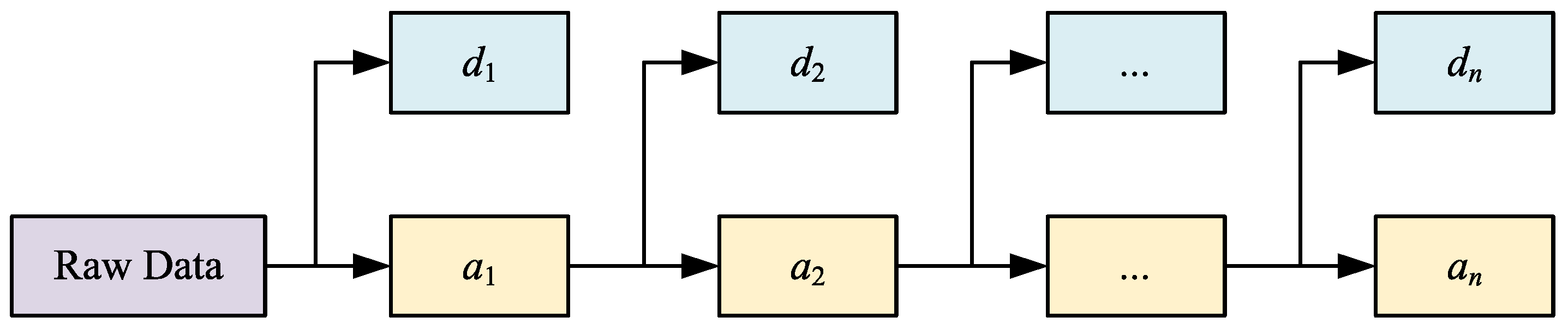
3.1. Wavelet Decomposition

Photovoltaic power generation and related environmental impact factors are time series with randomness and volatility, and wavelet decomposition can extract effective information from the time series [32]. Wavelet decomposition utilizes a series of basis functions called wavelets to represent signals, which are obtained by translating and scaling a mother wavelet. Unlike the Fourier transform, which uses sine and cosine waves as basis functions, the wavelet transform is localized and has clear starting and ending points in the time domain. This enables wavelet decomposition to better capture the local characteristics of signals and capture both time and frequency domain information from a given time series, effectively addressing the limitations of the Fourier transform in time information loss and non-stationary signal analysis.

The energy normalization coefficient of a wavelet must meet the following condition [33]:

$$C_{\psi }={\int }_{-\infty }^{+\infty }{\displaystyle \frac{{\left|\widehat{\psi }\left(\omega \right)\right|}^2}{\left|\omega \right|}}d\omega <\infty$$

(10)

where $\omega$ represents the position of a signal or wavelet function in the frequency domain and $|\widehat{\psi }{\left(\omega \right)|}^2$ represents the power spectral density of the wavelet function’s Fourier transform.

The definition of continuous wavelet transform is as follows [33]:

$$W_g(p,q)=〈g,{\psi }_{p,q}〉={\int }_{-\infty }^{+\infty }g\left(t\right)\psi \left({\displaystyle \frac{t-q}{p}}\right)dtp\ne 0$$

(11)

$${\psi }_{p,q}\left(t\right)={\displaystyle \frac{1}{\sqrt{p}}}\psi \left({\displaystyle \frac{t-q}{p}}\right)$$

(12)

where $g\left(t\right)$ represents the original signal or the signal to be analyzed, $\psi \left(t\right)$ is the wavelet mother function, and the mother wavelet can be transformed by scaling the variable p and shifting the variable q to obtain the continuous wavelet ${\psi }_{p,q}\left(t\right)$.

The wavelet transform reconstruction algorithm is shown in Equation (13):

$$g\left(t\right)=C_{\psi }^{-1}{\int }_{-\infty }^{+\infty }{\int }_{-\infty }^{+\infty }{W}_g(p,q){\psi }_{p,q}\left(t\right){\displaystyle \frac{dp}{|p^2|}}dq$$

(13)

For discrete signals, the discrete wavelet transform (DWT) is generally used. p and q also need to be discretized to obtain the discrete wavelet ${\psi }_{j,k}\left(t\right)$ as follows [34]:

$${\psi }_{j,k}\left(t\right)=p_0^{-j/2}\psi \left(p_0^{-j}t-k{q}_0\right)$$

(14)

where $p_0$ represents the fundamental scaling factor in the discrete wavelet transform, while $q_0$ denotes the fundamental translation factor. j is the discretional index of the scaling parameter, indicating the degree of stretching or compression of the wavelet function at the current scale. k is the discretional index of the translation parameter, representing the discrete position of the wavelet function along the time axis.

The discrete wavelet transform can be expressed as follows:

$$G(j,k)=\sum _{t=-\infty }^{\infty }g\left(t\right){\psi }_{j,k}\left(t\right)$$

(15)

The discrete wavelet transform can also be expressed using the Mallat algorithm as follows [35]:

$$a_j=a_{j+1}{h}_1;d_j=d_{j+1}{l}_{1}j=0,1,\dots ,n-1$$

(16)

where $h_1$ and $l_1$, respectively, represent the low-pass filter coefficient and the high-pass filter coefficient; $a_j$ and $d_j$, respectively, represent trend signals and detail signals. The subscript represents the number of wavelet decomposition layers.

After reconstruction, it is as follows:

$$a_j=a_{j+1}{h}_2+d_{j+1}{l}_{2}j=n-1,\dots ,1,0$$

(17)

where $h_2$ and $h_2$ are the dual operators of $h_1$ and $h_1$, respectively.

The transformation process is shown in Figure 2.

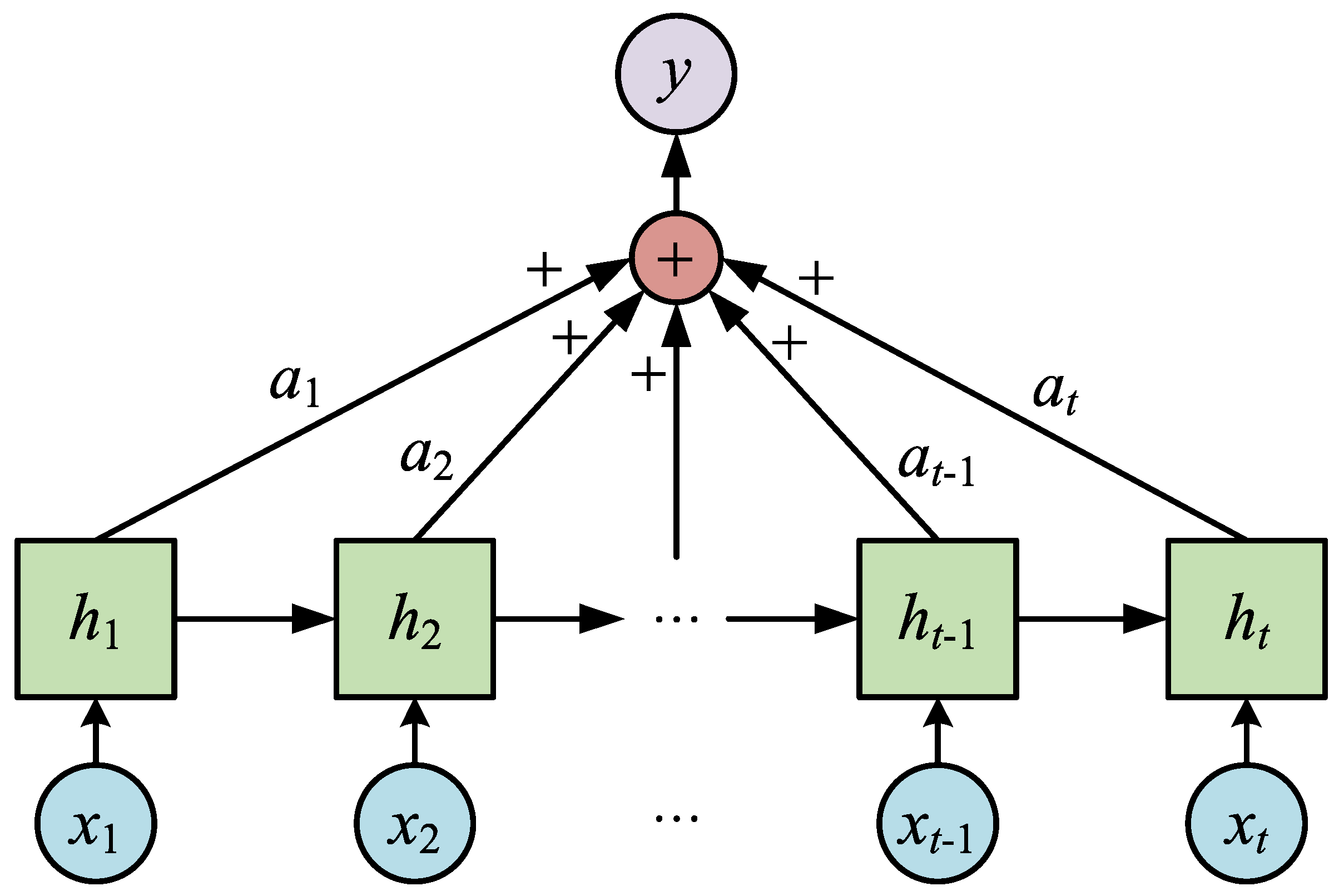
3.2. Dual Attention Mechanism

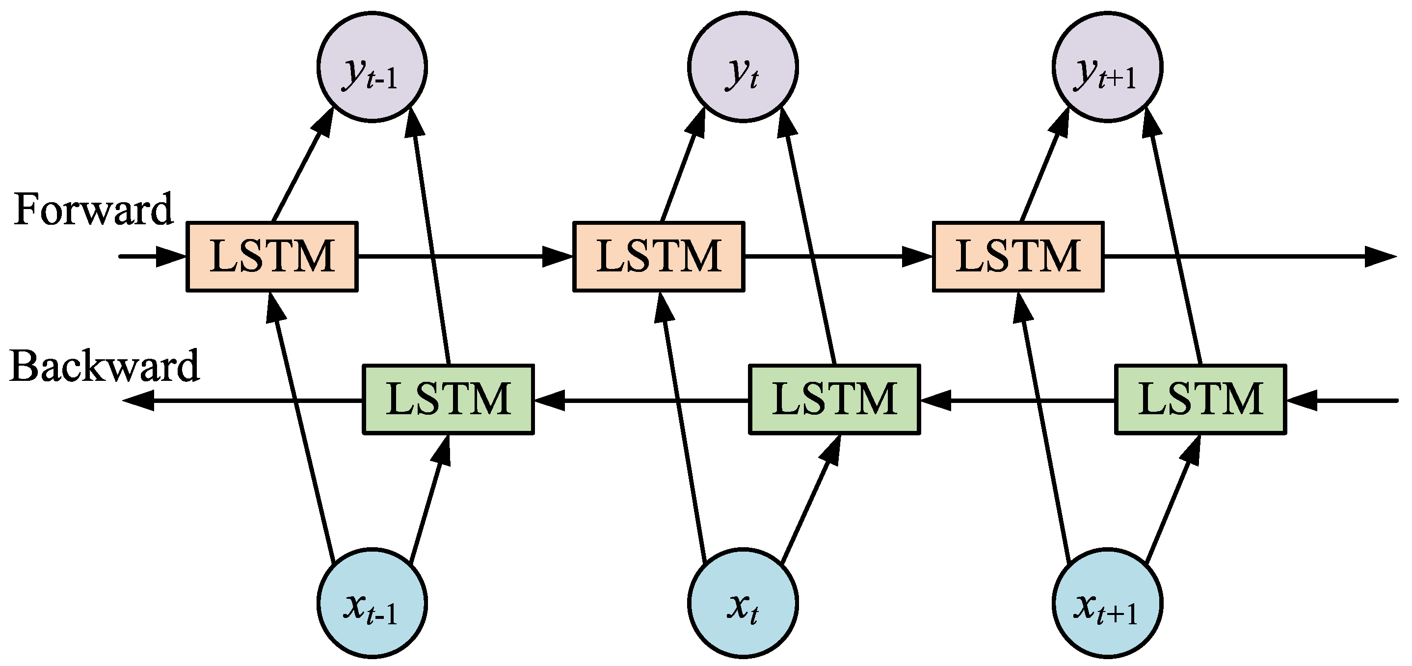
The power of photovoltaic power generation is influenced by various factors, such as solar irradiance, humidity, temperature, and time. The degree of influence of these factors is not static and unchanging, but changes with time, environmental conditions, and other external factors. Therefore, predictive models need to be able to dynamically identify and adapt to these changes in order to improve the accuracy of predictions. The attention mechanism is an effective tool for achieving this goal [36].

The attention mechanism simulates the attention pattern of the human brain on specific regions at a given moment by assigning different weights to hidden layer units in the neural network to highlight key information. This article integrates the attention mechanism into the prediction model, which can solve the problem of difficulty in capturing effective features when processing long time series, thereby strengthening the model’s ability to predict the trend of photovoltaic power generation changes. The principle of the attention mechanism is shown in Figure 3.

The formula for calculating the weight coefficients of the attention mechanism layer is as follows [36]:

$$z_t=vtanh(w{h}_t+b)$$

(18)

$$a_t={\displaystyle \frac{e^{z_t}}{{\sum }_{j=1}^T{e}^{z_j}}}$$

(19)

$$s_t=\sum _{t=1}^T{a}_t{h}_t$$

(20)

where $z_t$ represents the attention probability distribution value obtained from the output $h_t$ of the hidden layer at time step t; $a_t$ represents the attention weight at time step t; v, w represents the weight coefficient; b represents the bias amount; and $s_t$ represents the output at time t.

The dual attention (DA) mechanism is an extension and deepening of the single attention mechanism, which provides a more comprehensive data understanding ability for the model by simultaneously focusing on two different dimensions: time and features.

By introducing a feature attention (FA) mechanism on the input side, the model can automatically identify the influence relationship between environmental features and photovoltaic power generation by learning the weight distribution of input features. This relationship may change with weather conditions, and the feature attention mechanism enables the model to dynamically adapt to these changes. Introducing a temporal attention (TA) mechanism on the output side allows the long-term output of the model to be weighted in order to identify and highlight the most influential time points or time periods on the prediction results.

3.3. BiLSTM

BiLSTM arranges two LSTM layers in parallel, one processing the forward sequence and the other processing the reverse sequence, allowing the model to simultaneously capture the dependencies before and after in the time series. Compared with LSTM one-way information transmission from front to back, it has stronger feature acquisition ability and can improve prediction accuracy [37]. The principle of BiLSTM is shown in Figure 4.

According to the schematic diagram, BiLSTM includes forward computation and backward computation.The typical LSTM principle is quite classic, and will not be elaborated in this article.

4. Model Architecture

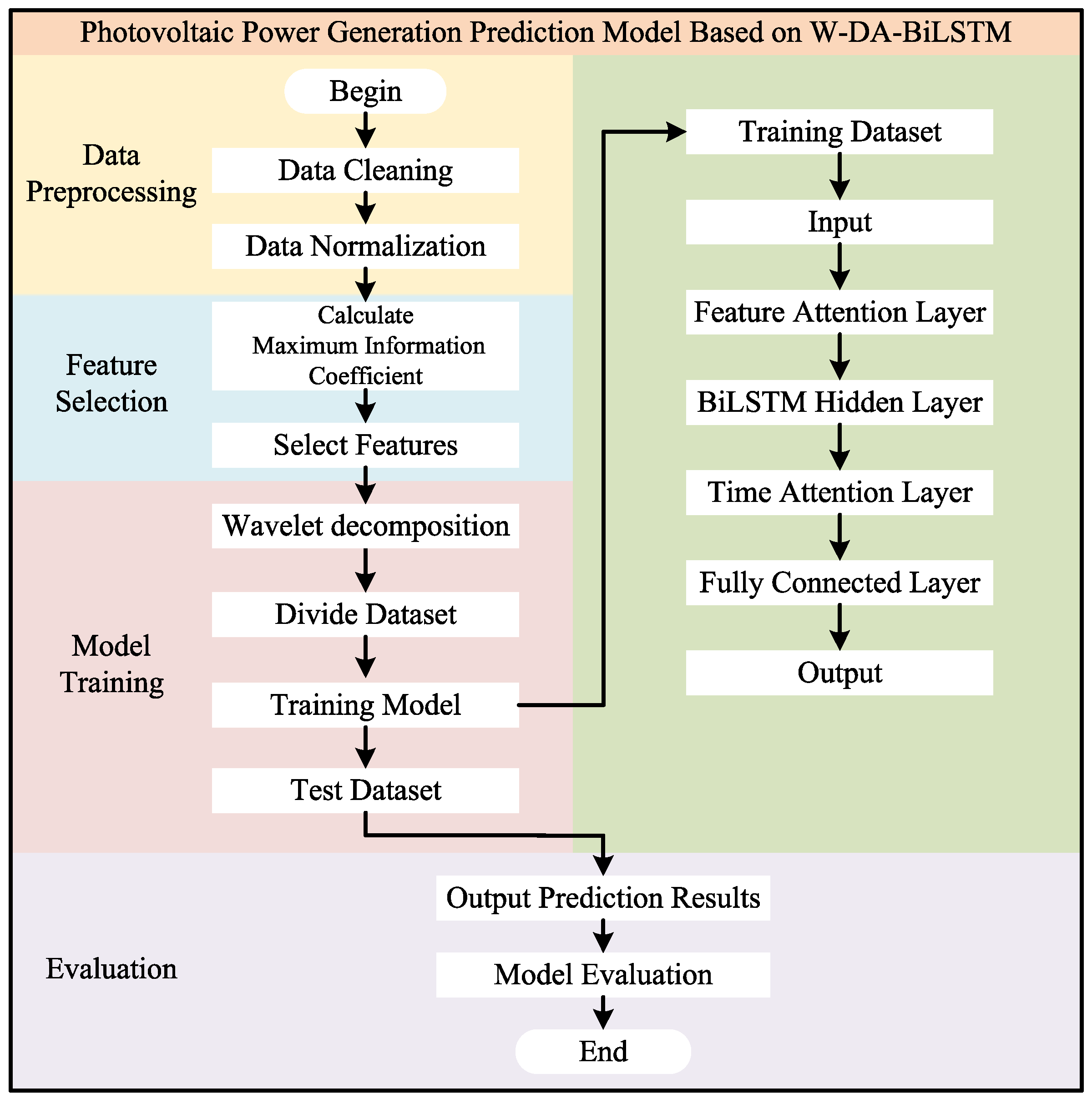
4.1. Algorithm Flow

The overall framework of the W-DA-BiLSTM model structure is shown in Figure 5.

The specific steps are as follows:

• Data preprocessing: clean the raw data, including outlier detection and removal and missing value completion, and then normalize the data to eliminate the influence of dimensionality.
• Feature selection: calculate the maximum information coefficient between each input, analyze the correlation between various factors, and then extract factors with a strong correlation with photovoltaic power generation.
  The definition of the maximum information coefficient is as follows [38]:

  $$I(X,Y)=\int p(X,Y){log}_2{\displaystyle \frac{p(X,Y)}{p\left(X\right)p\left(Y\right)}}dXdY$$

  (21)

  $$\mathrm{MIC}(X,Y)=\underset{a·b<B\left(n\right)}{max}{\displaystyle \frac{I(X,Y)}{{log}_{2}min(a,b)}}$$

  (22)

  $$B\left(n\right)=n^{0.6}$$

  (23)

  where X and Y are two input variables; I and p are the mutual information coefficient and joint probability between two variables, respectively; a and b are the number of grids divided in the X and Y directions; and $B\left(n\right)$ is the data range, usually set to the power of 0.6 of the total dataset.
  The maximum information coefficient value range is [0, 1]. When its value is 0, it indicates no correlation, and when it is 1, it indicates complete correlation. The stronger the correlation, the closer its value is to 1.
• Model training: perform wavelet decomposition and single-branch reconstruction on the filtered data, filter out noise, and then extract trend information.
• Model evaluation: use the trained prediction model to predict the test set, output the prediction results, and then evaluate the model using evaluation metrics.

4.2. Network Structure

The model based on wavelet decomposition, a dual attention mechanism, and a bidirectional long short-term memory network includes an input layer, feature attention layer [36], temporal attention layer [36], BiLSTM hidden layer [37], fully connected layer [39], and output layer.

• Input layer: uses the partitioned training set data as input for the model.
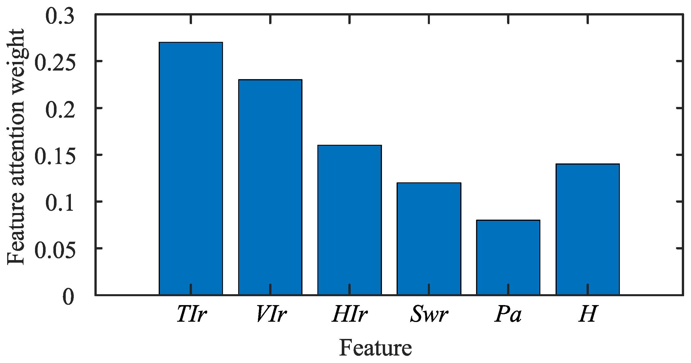
• Feature attention layer: learning the weight distribution of input data, the model can automatically identify the impact relationship between environmental features and photovoltaic power generation and enhance the influence of important features on prediction.
• BiLSTM hidden layer: processes forward and backward sequences to obtain the dependency relationship between them in the time series and combines the corresponding cell states in the forward and backward directions to obtain the output value at each time step.
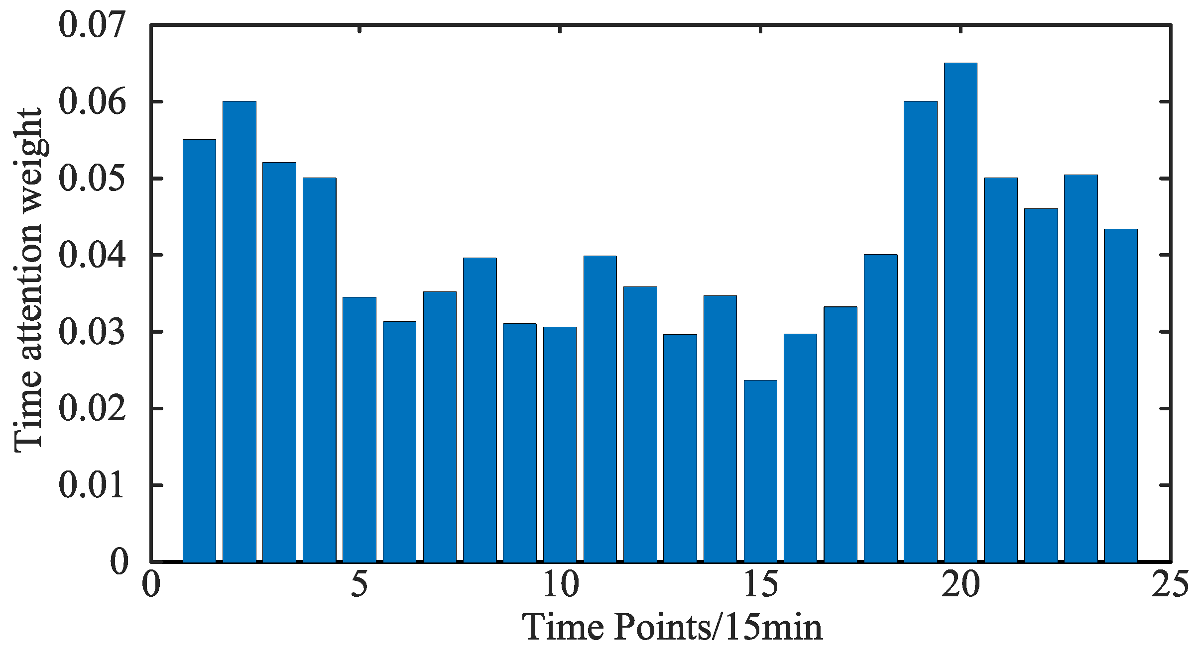
• Time attention layer: weights the sequence output of the model, highlighting the time points that have the most impact on the prediction results, and improves prediction accuracy through the temporal correlation between data.
• Fully connected layer and output layer: by reducing the dimensionality of the results through the fully connected layer and using the ReLU activation function to perform nonlinear mapping on the output data, the training speed can be improved and the final prediction results can be output.

5. Experiment

5.1. Experimental Data

The input data for the photovoltaic power generation model used in this article comes from measured data from a photovoltaic storage micro-grid in North China. The brief introduction of data information in the photovoltaic dataset is shown in

Table 1. Introduction to photovoltaic dataset.

Attribute	Value
Sampling interval	15 min
Time	From 0:00 on 1 January 2020 to 23:45 on 31 December 2020
Input factors	$Power$, $TIr$, $VIr$, $HIr$, T, $Pa$, H, $Swr$

. Here, Power is the photovoltaic power generation, $TIr$ is the total irradiance, $VIr$ is the normal direct irradiance, $HIr$ is the horizontal scattered irradiance, T is the temperature, $Pa$ is the atmospheric pressure, H is the relative humidity, and $Swr$ is the radiation flux.

In order to verify the universality of the model in each season, the dataset was divided into four sub datasets A, B, C, and D according to the season. The data from each quarter were selected for model training and validation, as shown in

Table 2. Dataset partitioning information.

Dataset	Training Dataset	Test Dataset	Time
A	3532	884	1 January to 15 February
B	3532	884	1 April to 15 May
C	3532	884	1 July to 15 August
D	3532	884	1 Octobert to 15 November

.

In order to better evaluate the performance of the model and detect its generalization ability, the dataset was divided into training and testing sets in a ratio of 8:2.

5.2. Parameter Settings

It is necessary to set the model parameters reasonably in order to improve the performance of the prediction model. The parameters of this model mainly include wavelet decomposition and hyper-parameters in neural networks. The specific parameter settings are shown in

Table 3. Parameter settings.

Parameters	Name	Value
Wavelet decomposition parameters	db	4
	level	4
Network parameters	Time step	24
	Hidden layer	32
	Number of iterations	100
	Learning rate	0.01
	Optimizer	Adam

.

The W-DA-BiLSTM photovoltaic power generation prediction model proposed in this article is built on the PyTorch deep learning framework. The hardware platform is an Intel (R) Core (TM) i7-6700HQ CPU @ 2.60 GHz, a 2.60 GHz processor, and the software platform is for a Windows 10 64-bit operating system, compiled using Python.

5.3. Evaluation Index

The evaluation indicators of the model reflect the deviation between the predicted value and the true value and are the key to measuring the performance of the model. For regression tasks such as photovoltaic power generation prediction, commonly used model evaluation indicators include Mean Absolute Error (MAE), Root Mean Square Error (RMSE), and the Coefficient of Determination (R-Square, $R^2$) [40]. In order to eliminate the influence of data dimensionality on evaluation values, this article normalizes the evaluation indicators NMAE [41], NRMSE [42], and N$R^2$ [43].

$$\mathrm{NMAE}={\displaystyle \frac{1}{n}}\sum _{i=1}^n\left|y_{\mathrm{real}}-y_{\mathrm{fore}}\right|$$

(24)

$$\mathrm{NRMSE}=\sqrt{{\displaystyle \frac{1}{n}}\sum _{i=1}^n{\left(y_{\mathrm{real}}-y_{\mathrm{fore}}\right)}^2}$$

(25)

$$\mathrm{N}{R}^2=1-{\displaystyle \frac{{(y_{\mathrm{real}}-y_{\mathrm{fore}})}^2}{{(y_{\mathrm{real}}-y_{\mathrm{mean}})}^2}}$$

(26)

where n is the number of data samples; i is the data sample number; $y_{\mathrm{real}}$ is the normalized actual value of the sample; $y_{\mathrm{fore}}$ is the normalized sample prediction value; and $y_{\mathrm{mean}}$ is the average of the normalized actual values.

5.4. Result

Multiple models were selected for comparative analysis to verify the advantages of the proposed prediction model in this paper. The models participating in the comparison were long short-term memory (LSTM), long short-term memory combined with an attention mechanism (LSTM Attention), and the Gate Recurrent Unit (GRU) algorithm. One day was randomly selected from each of the four seasons for photovoltaic power generation prediction and a prediction curve graph was obtained and compared with the actual data, as shown in Figure 6.

It can be intuitively seen from the predicted curve graph that, in spring, the fluctuation in photovoltaic power is not significant, and in a few periods, the photovoltaic power may suddenly decrease due to cloud cover and other factors. In summer, with sufficient sunlight and good weather conditions, there is almost no fluctuation in power, and the photovoltaic power generation is also the highest in this season of the year. In autumn, photovoltaic power fluctuates greatly, and the accuracy of prediction results decreases, resulting in higher photovoltaic power generation. Compared to other seasons, there is a significant decrease in photovoltaic power generation in winter, and the power generation period is shortened.

By training the model for different seasons, the red line representing the prediction results of the W-DA-BiLSTM photovoltaic power generation prediction model proposed in this paper coincides most with the blue line representing the actual photovoltaic power generation in all four seasons. At the same time, it can be seen that the overlap between the combined model and the actual value is better than that of a single model, and the overlap between the LSTM prediction curve and the actual value curve is better than that of GRU.

Using the spring, summer, autumn and winter time periods set for the four datasets A, B, C, and D in Table 2, the ratio of training set to test set of 8:2 and the model parameter settings in Table 3, the evaluation indicators of each model under the four datasets A, B, C, and D are shown in

Table 4. Comparison of performance evaluation indexes of photovoltaic power generation prediction model.

Method	Evaluation	A	B	C	D
W-DA-Bi-LSTM	NMAE	0.0078	0.0065	0.0215	0.0119
	NRMSE	0.0199	0.0189	0.0387	0.0263
	N$R^2$	0.9910	0.9932	0.9783	0.9889
LSTM-Attention	NMAE	0.0203	0.0158	0.0359	0.0246
	NRMSE	0.0369	0.0288	0.0583	0.0410
	N$R^2$	0.9802	0.9842	0.9549	0.9754
LSTM	NMAE	0.0404	0.0363	0.0467	0.0437
	NRMSE	0.0723	0.0589	0.0895	0.0819
	N$R^2$	0.9510	0.9547	0.9379	0.9470
GRU	NMAE	0.0393	0.0371	0.0532	0.0451
	NRMSE	0.0692	0.0635	0.1021	0.0872
	N$R^2$	0.9515	0.9530	0.9289	0.9411

.

The prediction accuracy of the GRU and LSTM models is poor, while LSTM Attention has improved accuracy due to the addition of the attention mechanism. The W-DA-BiLSTM model proposed in this paper has the best prediction performance. Compared with the LSTM Attention model, the NMAE of our model decreased by 61.6%, 58.9%, 40.1%, and 51.6% in the four seasons, and the NRMSE decreased by 46.1%, 34.4%, 33.6%, and 35.9%, respectively.

The training datasets of different seasons also have an impact on the prediction accuracy of the model. Under the training of dataset B in summer, the model obtained more accurate predictions compared to other seasons due to sufficient sunlight and better climate conditions; under the training of dataset C in autumn, due to the significant fluctuations in photovoltaic power generation and environmental factors, the prediction accuracy decreased compared to other seasons. In the proposed model, compared with autumn, the NMAE decreased by 63.7% and the NRMSE decreased by 48.6% in summer.

6. Analysis

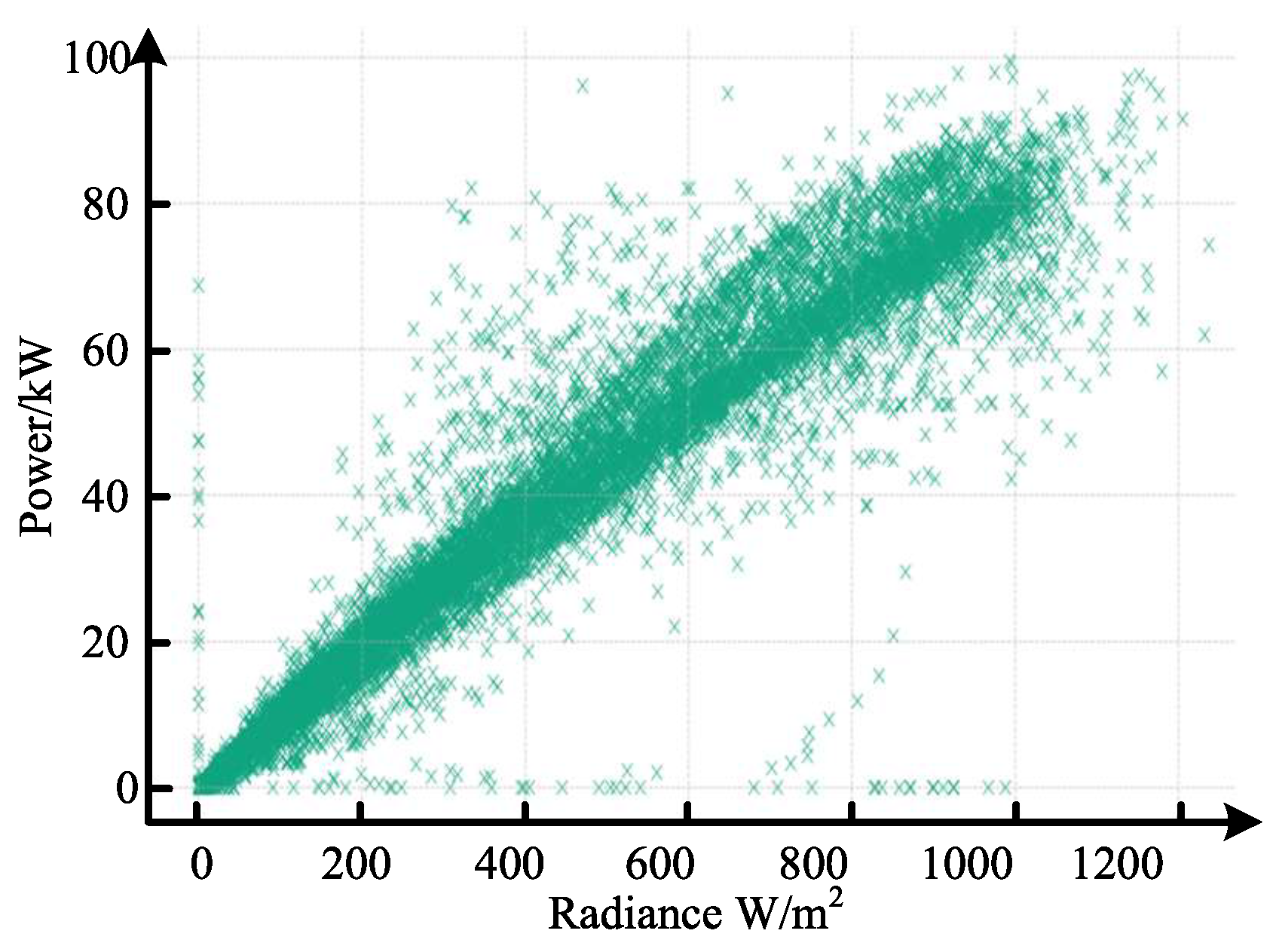
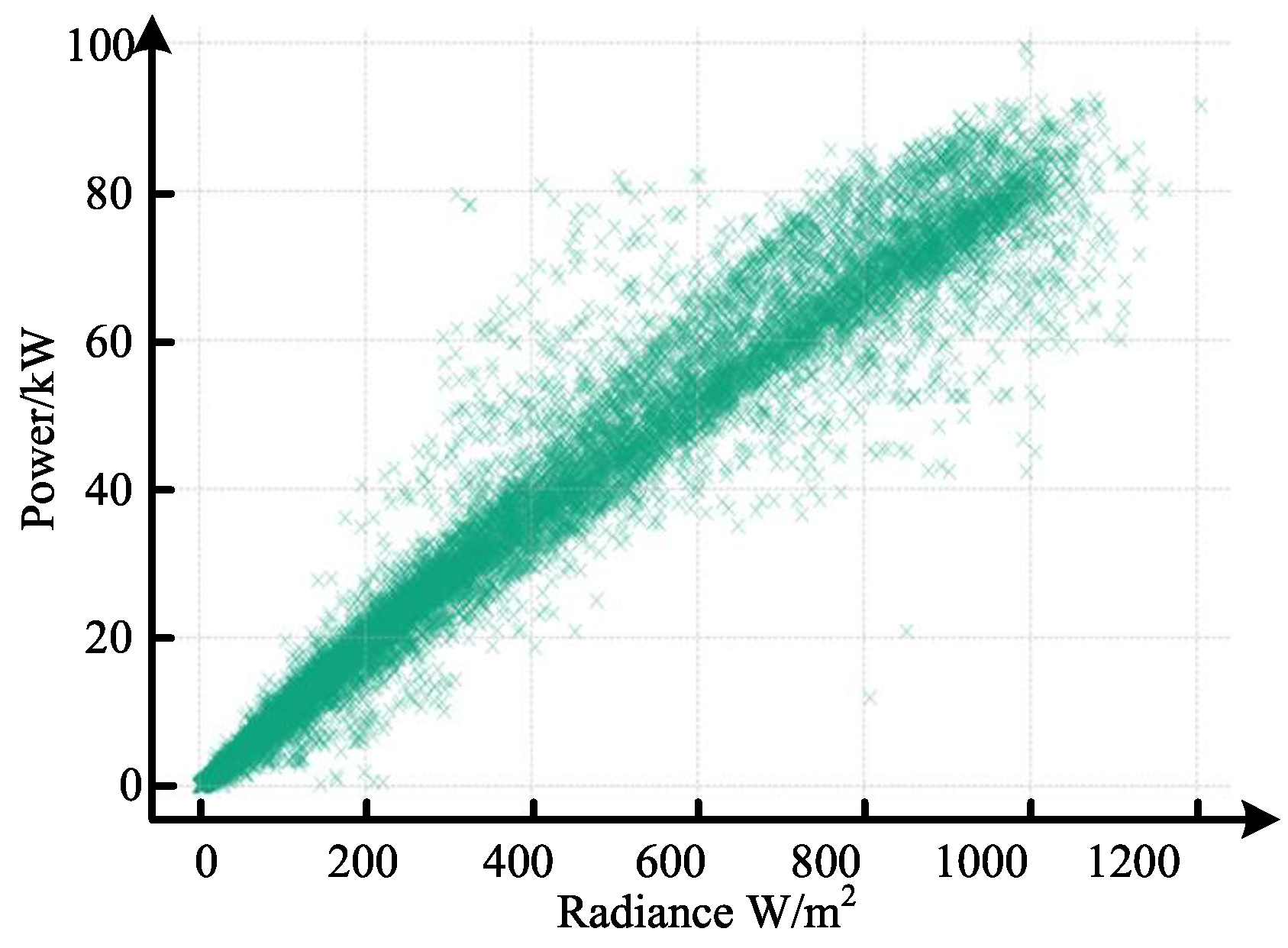
6.1. Analysis of Processing Results for Outliers and Missing Values

Figure 7 shows the relationship between photovoltaic power generation and total irradiance in the original dataset. This dataset includes a total of 35,136 sampling points, of which 35,120 points are valid and the remaining 16 points are missing. Although the proportion of missing values is small, they may cause computational issues during algorithm processing. In machine learning, missing values can affect the stability of results. From the graph analysis, it can be inferred that the trend of the dataset roughly follows the form of a power curve. However, some data points have significant deviations from the expected power curve of photovoltaic power generation, and these points are identified as outliers. Directly using these outliers can lead to model training being biased in the wrong direction, thereby weakening the model’s predictive ability.

After performing outlier detection, removal, and missing value interpolation on the photovoltaic dataset, a corrected scatter plot of photovoltaic power generation and irradiance was obtained, as shown in Figure 8.

By comparing the scatter plots before and after processing, it can be seen that the data distribution of the original photovoltaic dataset is relatively chaotic and has strong randomness. Figure 8 shows a more ordered data distribution, with a significant reduction in the number of outlier data points and a smoother power curve. In Figure 8, only a few outliers are concentrated in the region with zero power and its surroundings. It can be seen that the IQR abnormal data detection method can accurately identify and filter outliers while retaining the core part of the data. Meanwhile, the integrity and reliability of the dataset have been significantly improved through multiple imputation methods. Data cleaning eliminates the influence of outliers and missing values on model parameters, enhancing the predictive power of machine learning models. For photovoltaic system power prediction models, accurate relationships with variables such as irradiance are essential. Uncleaned outliers can cause the prediction curve to deviate from the actual operational data, thereby affecting system optimization and scheduling.

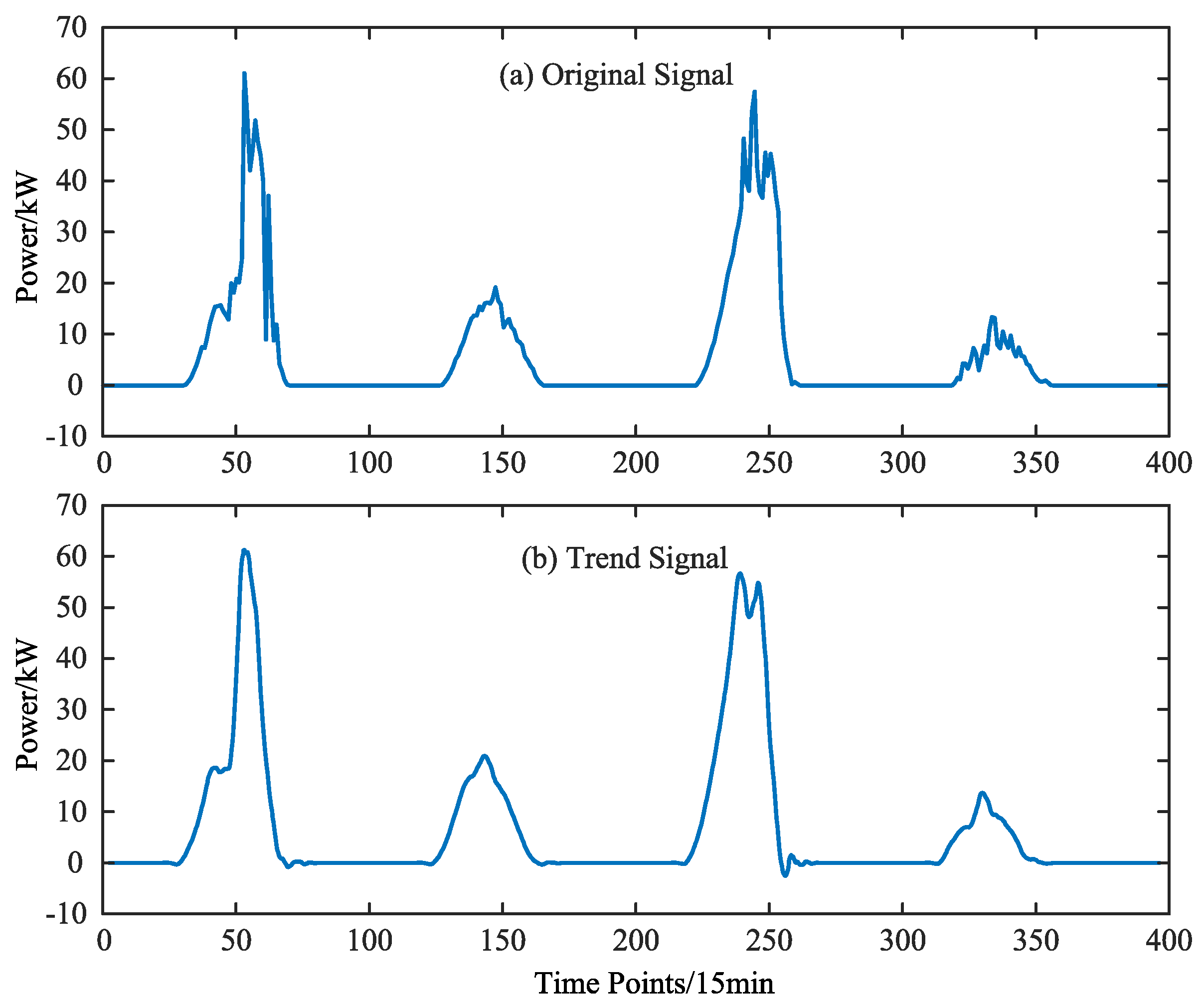
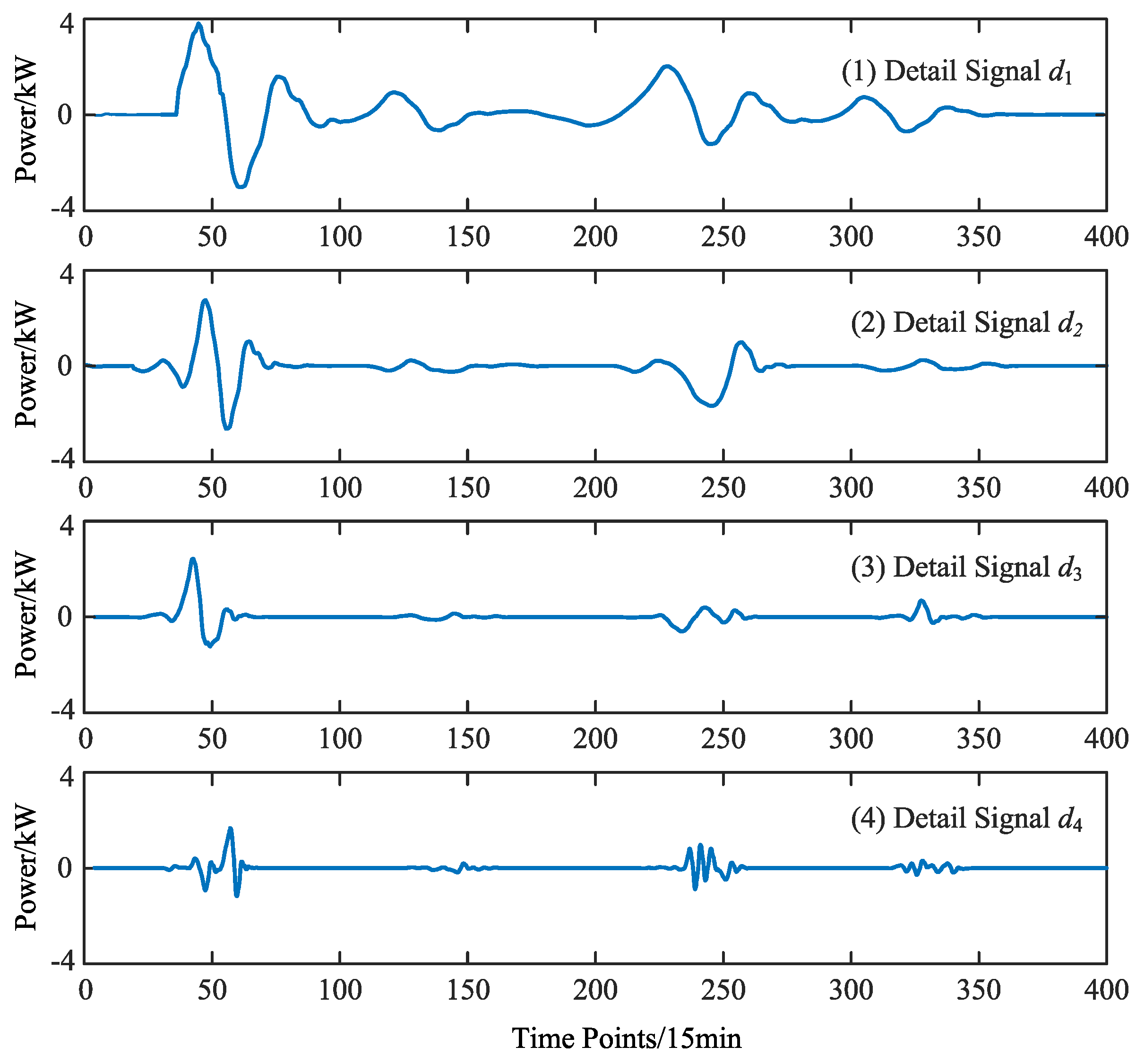
6.2. Analysis of Wavelet Decomposition Results

We randomly selected four-day photovoltaic power data for wavelet decomposition and single branch reconstruction, and obtained the signals shown in Figure 9 and Figure 10.

As shown in Figure 9, photovoltaic power generation is relatively high during the noon period of each day, and there are some fluctuations. Comparing the original signal and the trend signal, it can be seen that the trend changes of the two curves are basically the same, but the overall trend signal is smoother, which is due to the separation of the disturbance of detail signals in the trend.

Figure 10 shows the detailed signal. Wavelet decomposition of the original signal can separate small perturbation signals. Due to the use of $db4$ for wavelet decomposition, four frequency-increasing detail signals, $d1\text{–}d4$, are obtained.

By using wavelet decomposition to separate detailed signals and reduce their interference with trend signals during prediction, the accuracy of model prediction can be improved.

6.3. Analysis of the Results of Dual Attention Mechanism

The impact of different input features and time steps on photovoltaic power generation prediction varies. For different features, different weights are assigned through the feature attention mechanism, and the feature attention weight at a certain moment is shown in Figure 11.

For the three irradiance levels $TIr$, $VIr$, and $HIr$ with a high correlation with predicted power, they have higher weights when input into the model, and are the more critical information extracted by the feature attention mechanism for prediction.

The time attention weights for different time steps are shown in Figure 12. During steps 1 to 4 and steps 19 to 24, the attention span is relatively high, which is a more important step period for the prediction results. By utilizing attention mechanisms, the model can focus on critical time periods and enhance its ability to extract key information for prediction results.

7. Conclusions

• To improve the accuracy of photovoltaic power generation forecasting, this paper proposes a combined prediction model based on wavelet decomposition, dual attention mechanisms, and bidirectional long short-term memory networks (W-DA-BiLSTM). Simulation results using real-world data validate the model’s accuracy and effectiveness. The use of the quartile range method for outlier detection and the multiple interpolation method for missing value completion in data preprocessing improved the integrity and reliability of the dataset.
• Accurate ultra-short-term photovoltaic power forecasting is crucial for optimizing the scheduling strategies of photovoltaic-storage micro-grid systems. It ensures adequate power supply during peak demand periods while enabling low-cost energy storage during off-peak periods. This not only ensures the stable operation of the micro-grid but also maximizes economic benefits.
• The proposed prediction model achieves favorable forecasting results under various weather conditions. However, its accuracy under complex and extreme weather scenarios still has room for improvement. Further exploration of the factors affecting prediction accuracy under volatile weather conditions and potential enhancement strategies would be beneficial.

References

1. Liu, Y.; Chen, L.; Han, X. The key problem analysis on the alternative new energy under the energy transition. In Proceedings of the CSEE, Sanya, China, 25–27 February 2022; Volume 42, pp. 515–524. [Google Scholar]
2. Saeed, S.; Siraj, T. Global Renewable Energy Infrastructure: Pathways to Carbon Neutrality and Sustainability. Sol. Energy Sustain. Dev. J. 2024, 13, 183–203. [Google Scholar] [CrossRef]
3. Jaxa-Rozen, M.; Trutnevyte, E. Sources of uncertainty in long-term global scenarios of solar photovoltaic technology. Nat. Clim. Chang. 2021, 11, 266–273. [Google Scholar] [CrossRef]
4. Zhang, B.; Gao, Y. Data-driven voltage/var optimization control for active distribution network considering PV inverter reliability. Electr. Power Syst. Res. 2023, 224, 109800. [Google Scholar] [CrossRef]
5. Ibrahim, I.A.; Hossain, M.; Duck, B.C. An optimized offline random forests-based model for ultra-short-term prediction of PV characteristics. IEEE Trans. Ind. Inform. 2019, 16, 202–214. [Google Scholar] [CrossRef]
6. Wang, J.; Zhou, Y.; Li, Z. Hour-ahead photovoltaic generation forecasting method based on machine learning and multi objective optimization algorithm. Appl. Energy 2022, 312, 118725. [Google Scholar] [CrossRef]
7. Markovics, D.; Mayer, M.J. Comparison of machine learning methods for photovoltaic power forecasting based on numerical weather prediction. Renew. Sustain. Energy Rev. 2022, 161, 112364. [Google Scholar] [CrossRef]
8. Mayer, M.J.; Gróf, G. Extensive comparison of physical models for photovoltaic power forecasting. Appl. Energy 2021, 283, 116239. [Google Scholar] [CrossRef]
9. Lorenz, E.; Scheidsteger, T.; Hurka, J.; Heinemann, D.; Kurz, C. Regional PV power prediction for improved grid integration. Prog. Photovolt. Res. Appl. 2011, 19, 757–771. [Google Scholar] [CrossRef]
10. Perez, R.; Kivalov, S.; Schlemmer, J.; Hemker, K., Jr.; Renné, D.; Hoff, T.E. Validation of short and medium term operational solar radiation forecasts in the US. Sol. Energy 2010, 84, 2161–2172. [Google Scholar] [CrossRef]
11. Sheng, H.; Xiao, J.; Cheng, Y.; Ni, Q.; Wang, S. Short-term solar power forecasting based on weighted Gaussian process regression. IEEE Trans. Ind. Electron. 2017, 65, 300–308. [Google Scholar] [CrossRef]
12. Lamsal, D.; Sreeram, V.; Mishra, Y.; Kumar, D. Kalman filter approach for dispatching and attenuating the power fluctuation of wind and photovoltaic power generating systems. IET Gener. Transm. Distrib. 2018, 12, 1501–1508. [Google Scholar] [CrossRef]
13. Miao, S.; Ning, G.; Gu, Y.; Yan, J.; Ma, B. Markov Chain model for solar farm generation and its application to generation performance evaluation. J. Clean. Prod. 2018, 186, 905–917. [Google Scholar] [CrossRef]
14. Dong, J.; Olama, M.M.; Kuruganti, T.; Melin, A.M.; Djouadi, S.M.; Zhang, Y.; Xue, Y. Novel stochastic methods to predict short-term solar radiation and photovoltaic power. Renew. Energy 2020, 145, 333–346. [Google Scholar] [CrossRef]
15. Hocaoglu, F.O.; Serttas, F. A novel hybrid (Mycielski-Markov) model for hourly solar radiation forecasting. Renew. Energy 2017, 108, 635–643. [Google Scholar] [CrossRef]
16. Sun, X.; Qiu, J.; Tao, Y.; Ma, Y.; Zhao, J. A multi-mode data-driven volt/var control strategy with conservation voltage reduction in active distribution networks. IEEE Trans. Sustain. Energy 2022, 13, 1073–1085. [Google Scholar] [CrossRef]
17. Ahmed, A.; Khalid, M. A review on the selected applications of forecasting models in renewable power systems. Renew. Sustain. Energy Rev. 2019, 100, 9–21. [Google Scholar] [CrossRef]
18. Ghimire, S.; Deo, R.C.; Downs, N.J.; Raj, N. Global solar radiation prediction by ANN integrated with European Centre for medium range weather forecast fields in solar rich cities of Queensland Australia. J. Clean. Prod. 2019, 216, 288–310. [Google Scholar] [CrossRef]
19. VanDeventer, W.; Jamei, E.; Thirunavukkarasu, G.S.; Seyedmahmoudian, M.; Soon, T.K.; Horan, B.; Mekhilef, S.; Stojcevski, A. Short-term PV power forecasting using hybrid GASVM technique. Renew. Energy 2019, 140, 367–379. [Google Scholar] [CrossRef]
20. Behera, M.K.; Majumder, I.; Nayak, N. Solar photovoltaic power forecasting using optimized modified extreme learning machine technique. Eng. Sci. Technol. Int. J. 2018, 21, 428–438. [Google Scholar] [CrossRef]
21. Pan, C.; Tan, J. Day-ahead hourly forecasting of solar generation based on cluster analysis and ensemble model. IEEE Access 2019, 7, 112921–112930. [Google Scholar] [CrossRef]
22. Wang, K.; Qi, X.; Liu, H. Photovoltaic power forecasting based LSTM-Convolutional Network. Energy 2019, 189, 116225. [Google Scholar] [CrossRef]
23. Zhen, H.; Niu, D.; Wang, K.; Shi, Y.; Ji, Z.; Xu, X. Photovoltaic power forecasting based on GA improved Bi-LSTM in microgrid without meteorological information. Energy 2021, 231, 120908. [Google Scholar] [CrossRef]
24. Abdel-Basset, M.; Hawash, H.; Chakrabortty, R.K.; Ryan, M. PV-Net: An innovative deep learning approach for efficient forecasting of short-term photovoltaic energy production. J. Clean. Prod. 2021, 303, 127037. [Google Scholar] [CrossRef]
25. Shi, P.M.; Guo, X.Y.; Du, Q.C.; Xu, X.F.; He, C.B.; Li, R.X. Photovoltaic Power Prediction Based on TCN-BiLSTM-Attention-ESN. Acta Energiae Solaris Sin. 2024, 45, 304–316. [Google Scholar]
26. Huang, L.; Gan, H.Y.; Liu, X.J.; Kou, Z.; Li, J.; Wang, Y.H.; Gu, B. Ultra-short-term Photovoltaic Power Generation Prediction Based on Transformer Encoder. Smart Power 2024, 52, 16–23. [Google Scholar]
27. Huang, Z.; Bi, G.-H.; Xie, X.; Zhao, X.; Chen, C.P.; Zhang, Z.R.; Luo, Z. Ultra-short-term PV power prediction based on MBI-PBI-Res Net. Power Syst. Prot. Control 2024, 52, 165–176. [Google Scholar]
28. Swami, R.; Dave, M.; Ranga, V. IQR-based approach for DDoS detection and mitigation in SDN. Def. Technol. 2023, 25, 76–87. [Google Scholar] [CrossRef]
29. Frery, A.C. Interquartile Range. In Encyclopedia of Mathematical Geosciences; Springer: Berlin/Heidelberg, Germany, 2023; pp. 664–666. [Google Scholar]
30. Singh, K.; Upadhyaya, S. Outlier detection: Applications and techniques. Int. J. Comput. Sci. Issues (IJCSI) 2012, 9, 307. [Google Scholar]
31. Royston, P. Multiple imputation of missing values. Stata J. 2004, 4, 227–241. [Google Scholar] [CrossRef]
32. Zhao, P.; Tan, W.; Cao, S.; Liu, Y. Short term PV power generation prediction based on wavelet transform and LSTM. In Proceedings of the Eighth International Conference on Energy System, Electricity, and Power (ESEP 2023), Wuhan, China, 24–26 November 2023; SPIE: Bellingham, WA, USA, 2024; Volume 13159, pp. 191–197. [Google Scholar]
33. Pathak, R.S. The Wavelet Transform; Springer Science & Business Media: Berlin/Heidelberg, Germany, 2009; Volume 4. [Google Scholar]
34. Zhang, D. Wavelet transform. In Fundamentals of Image Data Mining: Analysis, Features, Classification and Retrieval; Springer: Cham, Switzerland, 2019; pp. 35–44. [Google Scholar] [CrossRef]
35. Nason, G.P.; Silverman, B.W. The discrete wavelet transform in S. J. Comput. Graph. Stat. 1994, 3, 163–191. [Google Scholar] [CrossRef]
36. Vaswani, A.; Shazeer, N.; Parmar, N.; Uszkoreit, J.; Jones, L.; Gomez, A.N.; Kaiser, L.; Polosukhin, I. Attention Is All You Need. arXiv 2017, arXiv:1706.03762. [Google Scholar]
37. Siami-Namini, S.; Tavakoli, N.; Namin, A.S. The performance of LSTM and BiLSTM in forecasting time series. In Proceedings of the 2019 IEEE International Conference on Big Data (Big Data), Los Angeles, CA, USA, 9–12 December 2019; IEEE: Washington, DC, USA, 2019; pp. 3285–3292. [Google Scholar]
38. Kinney, J.B.; Atwal, G.S. Equitability, mutual information, and the maximal information coefficient. Proc. Natl. Acad. Sci. USA 2014, 111, 3354–3359. [Google Scholar] [CrossRef] [PubMed]
39. Gao, Z. Stock Price Prediction Based on Joint LSTM and Fully Connected Layer. In Proceedings of the Recent Advancements in Computational Finance and Business Analytics: Proceedings of the 2nd International Conference on Computational Finance and Business Analytics-ICCFBA-2024, Bhubaneswar, India, 5–6 April 2024; Springer Nature: Berlin/Heidelberg, Germany, 2024; Volume 42, p. 109. [Google Scholar]
40. Chai, T.; Draxler, R.R. Root mean square error (RMSE) or mean absolute error (MAE). Geosci. Model Dev. Discuss. 2014, 7, 1525–1534. [Google Scholar]
41. Nespoli, A.; Ogliari, E.; Leva, S.; Massi Pavan, A.; Mellit, A.; Lughi, V.; Dolara, A. Day-ahead photovoltaic forecasting: A comparison of the most effective techniques. Energies 2019, 12, 1621. [Google Scholar] [CrossRef]
42. Ağbulut, Ü.; Gürel, A.E.; Biçen, Y. Prediction of daily global solar radiation using different machine learning algorithms: Evaluation and comparison. Renew. Sustain. Energy Rev. 2021, 135, 110114. [Google Scholar] [CrossRef]
43. Chicco, D.; Warrens, M.J.; Jurman, G. The coefficient of determination R-squared is more informative than SMAPE, MAE, MAPE, MSE and RMSE in regression analysis evaluation. Peerj Comput. Sci. 2021, 7, e623. [Google Scholar] [CrossRef] [PubMed]
Figure 1. Irradiance quantile–quantile chart.
Electronics 14 00306 g001
Figure 2. Wavelet transform process.
Electronics 14 00306 g002
Figure 3. Principle diagram of attention mechanism.
Electronics 14 00306 g003
Figure 4. BiLSTM schematic diagram.
Electronics 14 00306 g004
Figure 5. Structure diagram of W-DA-BiLSTM photovoltaic power generation prediction model.
Electronics 14 00306 g005
Figure 6. Comparison of forecast results in different seasons.
Electronics 14 00306 g006
Figure 7. Scatter plot of photovoltaic power generation and irradiance before processing.
Electronics 14 00306 g007
Figure 8. Scatter plot of photovoltaic power generation and irradiance after processing.
Electronics 14 00306 g008
Figure 9. Wavelet decomposition of raw signal and trend signal.
Electronics 14 00306 g009
Figure 10. The wavelet decomposes the detailed signal.
Electronics 14 00306 g010
Figure 11. Weight distribution of feature attention mechanism.
Electronics 14 00306 g011
Figure 12. Weight distribution of time attention mechanism.
Electronics 14 00306 g012