Depth Estimation Based on MMwave Radar and Camera Fusion with Attention Mechanisms and Multi-Scale Features for Autonomous Driving Vehicles

Abstract

Autonomous driving vehicles have strong path planning and obstacle avoidance capabilities, which provide great support to avoid traffic accidents. Autonomous driving has become a research hotspot worldwide. Depth estimation is a key technology in autonomous driving as it provides an important basis for accurately detecting traffic objects and avoiding collisions in advance. However, the current difficulties in depth estimation include insufficient estimation accuracy, difficulty in acquiring depth information using monocular vision, and an important challenge of fusing multiple sensors for depth estimation. To enhance depth estimation performance in complex traffic environments, this study proposes a depth estimation method in which point clouds and images obtained from MMwave radar and cameras are fused. Firstly, a residual network is established to extract the multi-scale features of the MMwave radar point clouds and the corresponding image obtained simultaneously from the same location. Correlations between the radar points and the image are established by fusing the extracted multi-scale features. A semi-dense depth estimation is achieved by assigning the depth value of the radar point to the most relevant image region. Secondly, a bidirectional feature fusion structure with additional fusion branches is designed to enhance the richness of the feature information. The information loss during the feature fusion process is reduced, and the robustness of the model is enhanced. Finally, parallel channel and position attention mechanisms are used to enhance the feature representation of the key areas in the fused feature map, the interference of irrelevant areas is suppressed, and the depth estimation accuracy is enhanced. The experimental results on the public dataset nuScenes show that, compared with the baseline model, the proposed method reduces the average absolute error (MAE) by 4.7–6.3% and the root mean square error (RMSE) by 4.2–5.2%.

1. Introduction

In recent years, autonomous driving technology has developed rapidly. Environmental perception is the basis for autonomous driving to avoid obstacles and plan paths [1,2]. Depth estimation plays a critical role in helping autonomous systems to accurately determine target distances and make informed decisions [3,4]. Depth estimation methods based on CNNs (Convolutional Neural Networks) [5] are widely used because they can effectively improve the accuracy of depth estimation. Current works [6,7,8] usually treat depth estimation as a regression problem. However, the accuracy of depth regression remains a challenge that requires further attention. Therefore, Refs. [9,10] proposed to combine multiple tasks for depth estimation to improve accuracy.

Among the various depth estimation methods, monocular depth estimation using a monocular camera has become a research hotspot due to its wide applicability. The research methods have evolved from supervised to unsupervised learning; however, the inherent limitation of monocular cameras in capturing depth information restricts the accuracy of depth estimation. To address this limitation, Refs. [11,12] proposed a depth estimation method that combines LiDAR (Light Detection and Ranging) and a camera and performed depth completion by introducing depth information from LiDAR data. However, LiDAR is greatly affected by weather and has high costs and computing power requirements [13]. Compared with LiDAR, automotive MMwave (millimeter-wave) radar not only provides depth information but also operates effectively under all weather conditions [14]. In addition, the amount of data generated by MMwave radar is smaller than that of LiDAR, as shown in Figure 1, which reduces the hardware requirements for edge devices [15,16]. Therefore, we introduce MMwave radar data to provide prior depth information. Considering the sparsity of MMwave radar point cloud data, we need to map the point cloud data and extract depth information and then fuse it with the image for depth estimation. The depth estimation process is shown in Figure 2.

Figure 1. Plotting LiDAR and millimeter-wave radar point clouds in images. (a) LiDAR point cloud projection. (b) Millimeter-wave radar point cloud projection.

Figure 2. Depth estimation using camera and millimeter-wave radar. (a) Input image. (b) Generating semi-dense depth estimation. (c) Generating dense depth estimation. Objects in the scene are highlighted with red box.

Depth estimation methods that fuse MMwave radar and camera data include data-level, decision-level, and feature-level fusion [17,18]. A comparison of the different fusion approaches by Lin et al. [19] indicates that feature-level fusion yields the best performance. This is because feature-level fusion enables radar depth features and image features to complement each other in a higher-level feature space and determines the depth value corresponding to the image area through the fusion process, thereby improving the depth estimation accuracy. Feature-level fusion is a new approach that has emerged in recent years and has become a research hotspot. Refs. [20,21] adopted the feature-level fusion approach. After fusing radar depth features and image features, depth estimation was completed through a regression network. However, these works do not establish the correlation between radar points and image regions, ignore the information loss problem in the feature fusion process, and lack the suppression of invalid regions when performing dense depth estimation. To solve these problems, we propose a depth estimation method based on MMwave radar and camera fusion with attention mechanisms and multi-scale features. The main contributions are as follows:

(i)

We fuse an image with a radar frame to obtain depth information, thereby avoiding the impact of data latency on depth estimation. By establishing correlations between radar points and image regions, we achieve semi-dense depth estimation results.

(ii)

For the fusion of the image and the semi-dense depth map, we propose an improved bidirectional multi-scale feature fusion structure as the lower-layer feature fusion method. This approach effectively utilizes feature information from different scales to solve the problem of information loss during the feature fusion process, enhancing the model’s robustness in complex scenes. Furthermore, by improving the loss function, the model achieves more stable backpropagation, leading to higher depth estimation accuracy.

(iii)

For the dense depth estimation stage, we propose a higher-layer feature fusion method using attention mechanisms. By using parallelly connected channel attention and spatial attention, we generate learnable attention weights to better utilize the global information from deeper layers and the local information from shallower layers. This enhances the representation of key regions, reduces the impact of redundant information, and improves the accuracy of depth estimation.

2. Related Work

2.1. Monocular Depth Estimation

Monocular depth estimation methods based on deep learning can automatically learn complex features, avoid manual feature extraction, and have gained increasing attention. Regarding supervised learning approaches, Eigen et al. [22] proposed a multi-scale network for depth prediction based on monocular image input. This method introduces the use of sparse depth labels obtained from LiDAR scans to train the depth prediction network. The algorithm uses a CNN to generate rough depth results and then restores the depth details. Subsequently, Eigen et al. [10] extended the original network by adding a third-scale network to enhance the image resolution. Laina et al. [23] utilized a deep residual network [24] to learn the mapping relationship between depth maps and single images. By employing a deep network for feature encoding and using an upsampling module as the decoder, they achieved high-resolution depth map outputs. Cao et al. [25] were the first to discretize depth values, transforming depth estimation into a pixel classification task rather than relying on depth continuity as in previous methods. Fu et al. [26] used regression networks for depth estimation and improved the accuracy of depth prediction by learning the sequential relationship between categories. Piccinelli et al. [27] proposed an internal discretization module for encoding internal feature representations in encoder–decoder network architectures, enhancing the generalization capability of depth estimation.

In unsupervised learning, Guizilini et al. [28] improved the network structure by employing 3D convolutions as the depth encoding–decoding network, replacing traditional pooling and upsampling operations. This approach better preserves object details in images. However, 3D convolutions significantly increase the number of network parameters, requiring more computational resources. Johnston et al. [29] proposed the use of self-attention and discrete depth to improve Monodepth2 [30]. Their approach employs ResNet101 as the depth encoder, achieving higher accuracy at the cost of a significantly increased parameter size. HR-Depth [31] introduces a nested dense skip connection design to obtain high-resolution feature maps, aiding in learning edge detail information. Additionally, a compression excitation block for feature fusion was proposed to enhance fusion efficiency. They also introduced a strategy for training a lightweight depth estimation network, achieving the performance of complex networks. FSRE-Depth [32] employs a metric-learning approach, leveraging semantic segmentation results to constrain the depth estimation, thereby improving the edge depth estimation. Additionally, a cross-attention module was designed to promote mutual learning and perception between the two tasks. Feng et al. [33] proposed a self-teaching unsupervised monocular depth estimation method. The student network is trained on lower-resolution enhanced images under the guidance of the teacher network. This method enhances the ability of the student network to learn effectively and improves the depth prediction accuracy.

2.2. Radar–Camera Depth Estimation

As radar point clouds are sparse, effectively fusing radar point clouds with images is a key research problem. Lin et al. [19] proposed a two-stage network based on a CNN to filter noise points in radar point clouds. The network takes radar data and images as the input. The first stage of the network filters out the noise points in the radar data, and the second stage of the network further refines the depth estimation results. Long et al. [21] proposed a radar-to-pixel association stage that learns the correspondence from radar-to-pixel mapping. They also used LiDAR point clouds for depth completion to obtain dense depth estimation. Both works employed multiple images or multiple radar frames (some images or radar frames belong to the next moment) for depth estimation instead of only using the scene image and radar frame at the current moment, which is unrealistic. Lo et al. [20] converted radar points into 3D measurements including height and then fused them with images. R4dyn [34] proposed a self-supervised depth estimation framework that utilizes radar as a supervisory signal to assist in dynamic object prediction in self-supervised monocular depth estimation. However, these works do not establish the correlation between radar points and image regions and ignore the impact of noise points in radar point clouds on depth estimation accuracy.

3. Materials and Methods

3.1. Overall Structure

We generate a dense depth estimation map from an image $I\in R^{3\times H\times W}$ and the corresponding millimeter-wave radar point cloud $P=\left\{p_n\right|p_n\in R^3,n=0,1,\dots ,N-1\}$, where H and W denote the height and width of the image, and N denotes the total number of radar points. As shown in Figure 1, although the millimeter-wave radar point cloud carries depth information, the radar points are mainly distributed in the horizontal range due to the inability to obtain accurate height data. This distribution differs significantly from that of LiDAR points. Furthermore, the presence of noisy radar points adds to the difficulty in determining the depth values of the image regions.

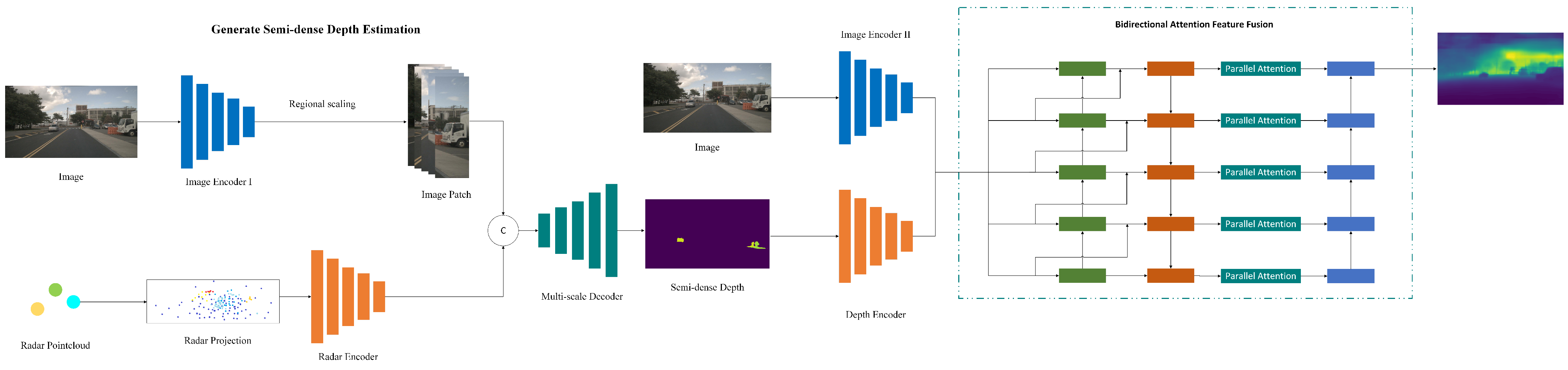
Our proposed overall framework is illustrated in Figure 3. Our method consists of three stages: (i) image features and radar features are obtained through different encoders. After concatenation, the combined features are processed through a decoder to generate a confidence map. This confidence map is used to assign depth values to image regions, resulting in a semi-dense depth estimation $S_d\in R^{H\times W}$. (ii) Image $I\in R^{3\times H\times W}$ and the semi-dense depth estimation $S_d\in R^{H\times W}$ are processed through encoders to obtain feature maps at different scales. These feature maps are then combined through a lower-layer bidirectional feature fusion to generate multi-scale fused feature maps. (iii) The multi-scale fused feature maps are processed through higher-layer parallel attention methods. Following successive upsampling, the dense depth estimation $D_d\in R^{H\times W}$ is generated.

Figure 3. Overall structure.

3.2. Generate Semi-Dense Depth Estimation

We obtain the semi-dense depth estimation $D_d\in R^{H\times W}$ by fusing an image and a radar frame. The image encoder is based on the residual network, with the image $I\in R^{3\times H\times W}$ used as input, and the numbers of output channels for each layer are 32, 64, 128, 128, and 128. After the co-ordinate transformation of the radar points, they are projected into the image co-ordinate system to generate a radar projection map. The value at each pixel position corresponding to a radar point in the radar projection map represents the depth information of the radar point. The radar encoder consists of 5 fully connected layers, with the number of channels for each layer being 32, 64, 128, 128, and 128. After passing through the radar encoder, the radar projection map produces radar feature maps with different numbers of channels.

To address the issue of missing precise height information in radar points and to expedite the correspondence between radar points and pixel regions, we scale the area of the true position of the radar points in the image to each feature map. This further allows us to obtain the ROI (Region of Interest) areas, ensuring that each ROI corresponds to the true location of the radar points. Then, it is necessary to establish correlation matching between the radar points and pixel regions. If an image corresponds to N radar points, it is necessary to output N confidence maps $C_i(I,p_n)\in {[0,1]}^{H\times W}$ to determine the image regions associated with each radar point. Each confidence map represents the probability that a pixel in I corresponds to a radar point $p_n$. Correspondence matching involves concatenating the feature maps of the image and the radar along the channel dimension. The concatenated feature maps are then processed by a decoder composed of successive upsampling and convolutional layers to produce the confidence maps. At this stage, each pixel $x_{hw}(h\in [0,H),w\in [0,W))$ in the image is associated with $p\in [0,N]$ radar points. Based on the confidence maps, radar points with confidence values exceeding a threshold are first selected for each pixel position. Then, the depth information of the radar point with the highest confidence is chosen as the depth estimate for each pixel position, resulting in the generation of a semi-dense depth estimation $S_d\in R^{H\times W}$:

$$S_d\left(I\right)=\left\{\begin{array}{c}\hfill d\left(p_n\right),C_n(I,p_n)(x_{hw},p_n)>\tau \\ \hfill 0,otherwise\end{array}\right.$$

(1)

where $n=arg\underset{i}{max}{C}_n(I,p_n)(x_{hw},p_n)$, $d\left(p_n\right)$ is the depth value corresponding to the pixel point and $\tau$ is the threshold value.

Loss Function

As some of the regions detected by LiDAR during the construction of the dataset may not be dense, this may result in a lack of supervised signals in these regions. For supervision, we chose to obtain the cumulative LiDAR depth $d_{acc}$ by projecting multiple LiDAR frames onto the current LiDAR frame $d_{gt}$. Pixel positions in $d_{acc}$ with a radar point depth difference within $0.4 \mathrm{m}$ were set to be in the positive class, thus constructing labels $y_{ld}\in {\{0,1\}}^{H\times W}$ for binary classification and minimizing the binary cross entropy loss:

$$L_{BCE}={\displaystyle \frac{1}{|\Omega |}}\sum _{x\in \Omega }-(y_{ld}\left(x\right)log{y}_c\left(x\right)+(1-y_{ld}\left(x\right))log(1-y_c\left(x\right)))$$

(2)

where $\Omega \subset R^2$ denotes the image region, $x\in \Omega$ denotes the pixel co-ordinates, and $y_c=C_i(I,p_n)$ denotes the confidence of the corresponding region.

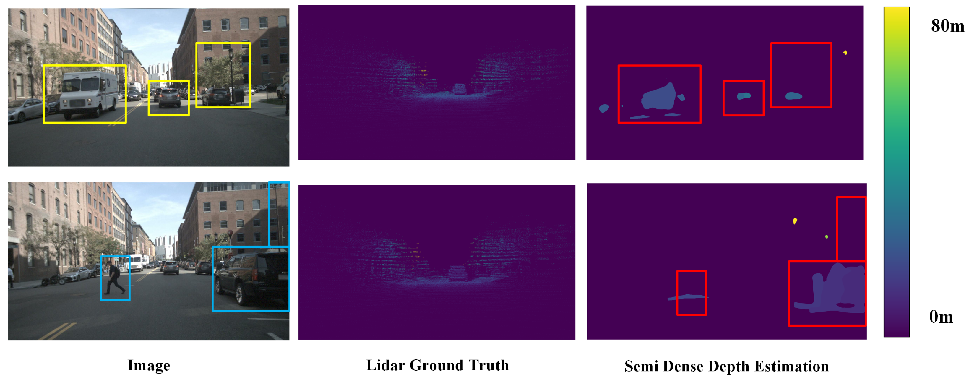
As shown in Figure 4, the first stage generates the semi-dense depth estimation $S_d$. On the far left is the original image, where yellow and blue boxes highlight significant areas. On the far right is the semi-dense depth estimation result, with preliminary depth estimation values assigned to the corresponding pedestrian or vehicle regions in the image.

Figure 4. Semi-dense depth estimation.Objects in the scene are highlighted with color boxes.

3.3. Lower-Layer Bidirectional Feature Fusion

To obtain a dense depth estimate from the semi-dense depth estimate, feature fusion between the semi-dense depth estimate and the image is required. Feature fusion is used to improve the information richness in features and combine the semantic information contained in features of different scales, which requires an understanding of the relationship between features of different scales. This is primarily based on two reasons: (i) it is difficult for the feature maps extracted by the convolutional layer to obtain both global and local information at the same time. Therefore, it is necessary to incorporate multi-scale information during the feature extraction process. (ii) Features at different levels may contain noise. Therefore, we propose a bidirectional feature fusion method so that features at different levels can better guide each other.

Using the image $I\in R^{3\times H\times W}$ and the semi-dense depth estimate $S_d\in R^{H\times W}$ as inputs to the feature encoder, the numbers of output channels for each layer are 16, 32, 64, 128, and 256. In order to suppress the background region, non-target region, and noise influence, the depth projection weight is generated through the depth feature map $D_f$ and then multiplied with the depth feature map to obtain the depth weight map $D_w$. The image feature map $I_f\in R^{c\times H\times W}$ and depth weight map $D_w\in R^{c\times H\times W}$ with the same number of channels c are added, and then they pass through the $1\times 1$ convolution layer to obtain $P_i$, where $i\in [1,5]$. The equation is as follows:

$$D_w=D_{f}Conv\left(D_f\right)$$

(3)

$$P_i=Conv(I_f+D_w)$$

(4)

As shown in Figure 5, the lower-layer feature fusion path starts from $F_5$. After $F_5$ undergoes upsampling and channel alignment, it is summed with $P_4$ to obtain the fused feature $F_4$. Subsequently, $F_3,F_2$ and $F_1$ are obtained through the same process. The equation is as follows:

$$F_i=Conv\left(UpSample\left(F_{i+1}\right)\right)+P_i$$

(5)

Figure 5. Bidirectional attention feature fusion structure.

To obtain more information about correlated regions during the fusion process, an additional input branch is introduced. After adding $F_1$ and $P_1$ to obtain $F_1^{\prime }$, $F_1^{\prime }$ is downsampled and channel-aligned, and then it is added to $F_2$ and $P_2$ to obtain $F_2^{\prime }$. The subsequent $F_3^{\prime }$ and $F_4^{\prime }$ are obtained through the same process. The equation is as follows:

$$F_i^{\prime }=Conv\left(F_i\right)+P_i,i=1$$

(6)

$$F_i^{\prime }=Conv\left(DownSamp\left(F_{i-1}\right)\right)+F_i+P_i,i\ge 2$$

(7)

3.4. Higher-Layer Attention Mechanism and Feature Fusion

As different channels have different importance, the channel attention mechanism is used to pay more attention to channels containing more important information and pay less attention to channels containing less important information, thereby improving feature representation capabilities [35].

As not all regions in the feature map are equally important in contributing to the model task, only regions relevant to the model task, such as the target object in a classification detection task, are of interest. The positional attention mechanism captures the spatial dependency of the feature map at any two locations by weighting all positional features and selectively aggregating features at each location, regardless of distance, and similar features are correlated with each other, thereby increasing the processing of correlated regions in different image layers in the fused feature map [36].

After the lower-layer bidirectional feature fusion, the fused feature maps at this stage retain abundant semantic information. In order to suppress the noise interference of irrelevant areas and enhance the multi-scale semantic information, we employ a parallel positional and channel attention mechanism for processing. The feature map obtained from $F_4^{\prime }$ after passing through the parallel attention modules is added to obtain $A_4$. After passing through the upsampling layer, $A_4$ is added to the feature map obtained by the parallel attention module of $F_3^{\prime }$ to obtain $A_3$. The subsequent $A_1$ and $A_2$ are obtained through the same process. After upsampling and convolution, $A_1$ produces the final dense depth estimation $D_d\in R^{H\times W}$ at the initial resolution. The equation is as follows:

$$A_i=Channel\left(F_i^{\prime }\right)+Position\left(F_i^{\prime }\right),i=4$$

(8)

$$A_i=Conv\left(UpSamp\left(A_{i+1}\right)\right)+Channel\left(F_i^{\prime }\right)+Position\left(F_i^{\prime }\right),1\le i\le 3$$

(9)

$$D_d=Conv\left(UpSamp\left(A_1\right)\right)$$

(10)

Loss Function

Ground truth depth $d_{gt}$ is obtained from the LiDAR point cloud, and $d_{acc}$ is obtained by accumulating LiDAR frames. During training, we minimize the difference between d, $d_{gt}$, and $d_{acc}$ by using a suitable $L1$ penalty:

$$L_{BAFF}={\lambda }_{acc}{l}_{acc}(d_{acc},D_d)+{\lambda }_{gt}{l}_{gt}(d_{gt},D_d)$$

(11)

$$l(d,D_d)=\left\{\begin{array}{c}\hfill {\displaystyle \frac{1}{|\Omega |}}\sum _{x\in \Omega }\left(\right|d\left(x\right)-D_d{\left(x\right)\left|\right)}^2/2,|d\left(x\right)-D_d\left(x\right)|<1\\ \hfill {\displaystyle \frac{1}{|\Omega |}}\sum _{x\in \Omega }\left(\right|d\left(x\right)-D_d\left(x\right)|-0.5),otherwise\end{array}\right.$$

(12)

where $\Omega \subset R^2$ denotes the image region with valid values; $x\in \Omega$ denotes the pixel co-ordinates; the weight coefficient ${\lambda }_{acc}$ is set to 1; and ${\lambda }_{gt}$ is set to 1.

3.5. Parallel Attention Mechanism

3.5.1. Channel Attention

The attention structure is shown in Figure 6. Taking the feature map $F\in R^{C\times H\times W}$ as input, it is transformed into matrix $M_1\in R^{C\times N}$, where $N=H\times W$ denotes the number of pixels. Then, after transposing matrix $M_1$ to obtain $M_2\in R^{N\times C}$, it is multiplied by matrix $M_1$ and passed through the softmax function to obtain the channel attention matrix $M_{CA}^{ij}\in R^{C\times C}$:

$$M_{CA}^{ij}={\displaystyle \frac{exp(M_1^i\times M_2^j)}{{\sum }_{i=1}^{C}exp(M_1^i\times M_2^j)}}$$

(13)

where $M_{CA}^{ij}$ denotes the degree of association between the ith and jth channels. The channel attention matrix $M_{CA}^{ij}$ is transformed into $R^{C\times H\times W}$ by multiplying it with matrix $M_1$, which is weighted by $\alpha$, and then it is added to F to obtain the channel attention feature map $F_{CA}\in R^{C\times H\times W}$:

$$F_{CA}=\alpha (M_{CA}^{ij}\times M_1)+F$$

(14)

where $\alpha$ is the learnable weight of the channel semantic information weighting feature, initialized to 0. $F_{CA}$ is a feature map that contains semantic dependencies between channels, which helps in accurate depth estimation.

Figure 6. Channel attention.

3.5.2. Position Attention

The attention structure is shown in Figure 7. Taking the feature map $S\in R^{C\times H\times W}$ as input, $B,C,D\in R^{C\times H\times W}$ are obtained by passing through three convolutional layers each; then, $B,C,D$ are transformed into matrices $M_b\in R^{N\times C},M_c\in R^{C\times N},M_d\in R^{N\times C}$, where $N=H\times W$. The matrices $M_b$ and $M_c$ are multiplied together and then processed by the softmax function to obtain the positional attention matrix $M_{PA}^{ij}\in R^{N\times N}$:

$$M_{PA}^{ij}={\displaystyle \frac{exp(M_b^i\times M_c^j)}{{\sum }_{i=1}^{N}exp(M_b^i\times M_c^j)}}$$

(15)

where $M_{PA}^{ij}$ denotes the degree of association between the ith and jth positions. The channel attention matrix $M_{PA}^{ij}$ is transformed into $R^{C\times H\times W}$ by multiplying it with matrix $M_d$, which is weighted by $\beta$, and then it is added to S to obtain the position attention feature map $S_{PA}\in R^{C\times H\times W}$:

$$S_{PA}=\beta (M_{PA}^{ij}\times M_d)+S$$

(16)

where $\beta$ denotes the learnable weight of the position information weighted feature, initialized to 0. $S_{PA}$ is a feature map containing the global position information of the image, which helps to locate the target area.

Figure 7. Position attention.

4. Experiments

4.1. Datasets and Experimental Environment

We used the nuScenes dataset [37] for model training and validation. This dataset includes 1000 scenes, capturing various driving conditions (including rainy, nighttime, and foggy scenarios). The data collection vehicles used various sensors, including MMwave radar, cameras, and LiDAR, with data collected in the Boston and Singapore areas. Each scene lasts for 20 s, containing 40 keyframes and corresponding radar frames, with each image having a resolution of 1600 × 900, totaling approximately 40,000 frames. To use the nuScenes dataset [37], we divided it into a training set with 750 scenes, a validation set with 150 scenes, and a test set with 150 scenes.

The experimental environment of this study is shown in Table 1.

Table 1. Experimental environment.

Experimental Platform	Environment Configuration
Operating systems	Ubuntu18.04
Programming Languages	Python 3.8
CPU	Intel(R) Xeon(R) Platinum 8352V
GPU	NVIDIA RTX A5000
CUDA	11.3

4.2. Training Details and Evaluation Metrics

For training with nuScenes [37], we take the LiDAR frame corresponding to the given image as $d_{gt}$, and we project the previous 80 LiDAR frames and the subsequent 80 LiDAR frames onto the current LiDAR frame $d_{gt}$ to obtain the accumulated LiDAR frame $d_{acc}$, during which dynamic objects are removed. We create binary classification labels $y={\{0,1\}}^{H\times W}$ from $d_{acc}$, where points with a depth difference of less than 0.4 m from the radar points are labeled as positive. $d_{gt}$, $d_{acc}$, and y are all used for supervision.

In the first stage of training, the input image size is 900 × 1600, and the cropped size during the ROI region extraction is set to 900 × 288. We use the Adam optimizer with $\beta$1 = 0.9, $\beta$2 = 0.999, and a learning rate of 2 × 10⁻⁴ for 70 epochs. Our data augmentation methods include horizontal flipping and adjustments to saturation, brightness, and contrast, each with a probability of 0.5.

In the second stage of training, we use the Adam optimizer with $\beta$1 = 0.9 and $\beta$2 = 0.999. We set the initial learning rate to 2 × 10⁻⁴ and train for 200 epochs, and then we reduce it to 1 × 10⁻⁴ and train for 200 epochs. The data augmentation methods include horizontal flipping and adjustments to saturation, brightness, and contrast, each with a probability of 0.5.

The error metrics that we use are some of those widely used in the literature for evaluating depth estimation, including the mean absolute error (MAE) and root mean square error (RMSE):

$$\mathrm{MAE}={\displaystyle \frac{1}{|\Omega |}}\sum _{x\in \Omega }|D_{d_{gt}}-D_d\left(x\right)|$$

(17)

$$\mathrm{RMSE}=\sqrt{{\displaystyle \frac{1}{|\Omega |}}{\sum }_{x\in \Omega }{|D_{d_{gt}}-D_d\left(x\right)|}^2}$$

(18)

4.3. Ablation Studies

In the ablation experiment, we added each module in turn for comparison and finally progressed to the method we proposed. The ablation experiment results are shown in Table 2. “BF“ indicates bidirectional feature fusion, “CA” indicates channel attention, and “PA“ indicates position attention. When the BF module is used to reduce the information loss in the fusion process of image features and deep features, MAE is reduced by 1.1% and RMSE is reduced by 1.9%. On this basis, in order to suppress the influence of invalid areas, we enhance the feature expression of key areas from two levels: channel dimension and spatial position. After adding CA and PA modules, respectively, MAE was reduced by 0.8% and 1.2%, and RMSE was reduced by 0.9% and 1.6%. Finally, the BF, CA, and PA modules are added at the same time. Experimental results show that the proposed method reduces MAE by 4.7% and RMSE by 4.2%, effectively improving the depth estimation accuracy.

Table 2. Results of ablation studies.

Method	MAE↓	RMSE↓
Baseline	1727.4	3746.8
+BF	1708.8	3672.6
+BF+CA	1693.5	3641.4
+BF+PA	1681.2	3616.8
+BF+CA+PA (Ours)	1646.5	3589.3

4.4. Comparison and Analysis of Results

As shown in Table 3, we compare our method with the existing methods at depths of 50 m, 70 m, and 80 m, as shown in Table 1. Compared with RC-PDA [21], our method reduced the MAE by 26%, 41.6%, and 44.7%, and it reduced the RMSE by 13.6%, 31.7%, and 39.4%. Compared with DORN [20], our method reduced the MAE by 14.5%, 18.4%, and 16.8%, and it reduced the RMSE by 12.9%, 12.8%, and 16.1%. Overall, compared with the baseline model, our method reduced the MAE by 4.7%, 6.3%, and 5.8% and reduced the RMSE by 4.2%, 5.2%, and 4.9%.

Table 3. Comparison of experimental results.

Eval Distance	Method	Radar Frames	Images	MAE↓	RMSE↓
50 m	RC-PDA [21]	5	3	2225.0	4156.5
	RC-PDA with HG	5	3	2315.7	4321.6
	DORN [20]	5 (×3)	1	1926.6	4124.8
	Singh [38]	1	1	1727.7	3746.8
	Ours	1	1	1646.5	3589.3
70 m	RC-PDA [21]	5	3	3326.1	6700.6
	RC-PDA with HG	5	3	3485.6	7002.9
	DORN [20]	5 (×3)	1	2380.6	5252.7
	Singh [38]	1	1	2073.2	4825.0
	Ours	1	1	1942.6	4574.1
80 m	RC-PDA [21]	5	3	3713.6	7692.8
	RC-PDA with HG	5	3	3884.3	8008.6
	DORN [20]	5 (×3)	1	2467.7	5554.3
	Lin [19]	3	1	2371.0	5623.0
	R4Dyn [34]	4	1	N/A	6434.0
	Sparse-to-dense [39]	3	1	2374.0	5628.0
	PnP [40]	3	1	2496.0	5578.0
	Singh [38]	1	1	2179.3	4898.7
	Ours	1	1	2052.9	4658.7

As shown in Figure 8, we plotted the MAE and RMSE curves of the different methods during the model training phase to verify the effectiveness of the proposed method.

Figure 8. Comparison of MAE and RMSE during training using different methods. MAE curve on the left and RMSE curve on the right.

4.4.1. Results Analysis

The results obtained via our method are shown in Figure 9. To compare the specific inference results, we illustrated the dense depth estimation results obtained with our methods alongside those obtained via other methods on nuScenes, as shown in Figure 10. We selected two representative traffic scenarios: one is a multi-vehicle road scene, and the other is a pedestrian crossing an intersection. In the first column, we highlighted the prominent parts of the images using yellow and blue boxes.

Figure 9. The first column is the input image; the second column is the LiDAR ground truth; the third column is the result of our method. Different-colored bounding boxes are used to mark prominent areas in the image.

Figure 10. The first column is the result of our method; the following columns represent the inference results of different methods. Red boxes are used to mark prominent areas in the image.

In the first row, RC-PDA [21] and DORN [20] only managed to capture blurry shapes of the vehicles on the left and in the middle, with the vehicle edges being indistinguishable from the background. While Singh et al. [38] could distinguish the shape of the vehicles, the edge delineation was not smooth enough, resulting in discontinuous edges in the area of the vehicle on the right. Our method, however, not only distinguished the vehicle shapes more effectively but also provided more detailed edge delineation, reducing edge discontinuities.

In the second row, the middle pedestrian is situated in a light–dark junction area, the vehicle on the right side of the scene is in a shadowed area, and there is a pole in the upper right corner. RC-PDA [21] and DORN [20] failed to capture the position of the pole, and the shapes of the middle pedestrian and the vehicle on the right were also blurry. Although Singh et al. [38] detected the pole’s position, the shape was not fully rendered. Our method provided a more complete shape and edge representation for the vehicle on the right, showed detailed depictions of both the torso and limbs of the pedestrian, and clearly captured and represented the position and shape of the pole.

In general, RC-PDA [21] and DORN [20] have poor depth estimation performance at larger ranges (80 m). Singh et al. [38] have insufficient edge distinction between target and background areas. Our method not only effectively improves the depth estimation accuracy in this range but also captures clear target shapes.

4.4.2. Regional Result Analysis

We selected specific areas from the result images for a regional comparison, as shown in Figure 11. The first row displays the vehicle regions obtained via our method and other methods, which we refer to as Region-1. It is evident that the vehicle shapes obtained via our method are much clearer. The second row shows the multi-object regions, which include vehicles, trees, and street lamps, and we call this Region-2. Our method not only provides clearer object shapes but also smoother edges. We compared our method with the existing methods regarding the depth range in Region-1 and Region-2, as shown in Table 4. The results demonstrate that our method consistently outperforms the other methods across different regions.

Figure 11. The first column is the input image; the second column is the regional result of our method; the following columns represent the regional results of different methods. Regions in different colors are used to distinguish depths within the image.

Table 4. Comparison of regional results.

Region	Method	MAE↓	RMSE↓
Region-1	RC-PDA [21]	24.46	41.15
	DORN [20]	23.71	39.87
	Singh [38]	22.84	39.42
	Ours	22.61	39.17
Region-2	RC-PDA [21]	28.86	49.95
	DORN [20]	28.64	49.76
	Singh [38]	27.57	49.27
	Ours	27.31	49.08

5. Conclusions

In order to enhance the performance of autonomous driving, particularly in terms of depth estimation, we propose a depth estimation method based on radar and cameras using attention mechanisms and multi-scale feature fusion. Firstly, to address the sparsity of radar point cloud data, we project radar points onto images through co-ordinate transformation. By learning the correlations between radar points and image regions, we establish the correspondence between radar points and image pixels. This enables the model to concentrate on target regions, assign initial depth values, and generate semi-dense depth estimations. Secondly, to further refine the depth estimation results, we re-encode the image and the semi-dense depth map. By improving the bidirectional multi-scale feature fusion structure, an additional image fusion pathway is introduced. This effectively leverages feature information at different scales, enhancing the richness and accuracy of feature representation. It also addresses the issue of information loss during feature fusion, thereby improving the model’s robustness in complex scenarios. Finally, unlike other methods that rely on the use of conventional convolutional layers as decoders for depth estimation, we employ a parallel attention mechanism to process the fused feature maps. This enhances the representation of target regions, effectively suppresses the influence of irrelevant areas and noise on the depth estimation results, and significantly improves depth estimation accuracy.

Compared with the baseline model, our method demonstrates significant performance improvements across various evaluation metrics. Within a 50 m range, the MAE is reduced by 4.7%, and the RMSE is reduced by 4.2%. For longer ranges of 70 m and 80 m, the MAE is reduced by 6.3% and 5.8%, respectively, while the RMSE is reduced by 5.2% and 4.9%, respectively. These results indicate that our method outperforms the baseline model in depth estimation across various scenarios regarding the nuScenes dataset. It effectively handles differences in shape, size, and other attributes of targets in diverse scenes, exhibiting excellent generalization capabilities.

Moreover, to ensure that the model can effectively perform in practical applications, it is essential to account for the limitations of real-world deployment platforms, such as the demands of depth estimation tasks or complex environmental conditions. Considering the importance of lightweight models for autonomous driving, we plan to adjust the model in the future, such as using an image encoder with shared parameters to reduce the model size; using a bidirectional attention feature fusion structure to replace the first-stage decoder to improve model accuracy and change it to a one-stage model; and removing unnecessary convolutional layers through model pruning to ensure that the model accuracy is maintained while improving the real-time performance of the model. Finally, we will deploy it in a test scenario and evaluate its performance in real-world applications. Insights from these test results will guide the subsequent refinement of the model design.

References

- Jiang, Y.; Wu, Y.; Zhang, J.; Wei, J.; Peng, B.; Qiu, C.W. Dilemma in optical identification of single-layer multiferroics. Nature 2023, 619, E40–E43. [Google Scholar] [CrossRef] [PubMed]
- Jiang, Y.; He, A.; Zhao, R.; Chen, Y.; Liu, G.; Lu, H.; Zhang, J.; Zhang, Q.; Wang, Z.; Zhao, C.; et al. Coexistence of photoelectric conversion and storage in van der Waals heterojunctions. Phys. Rev. Lett. 2021, 127, 217401. [Google Scholar] [CrossRef] [PubMed]
- Jiang, Y.; He, A.; Luo, K.; Zhang, J.; Liu, G.; Zhao, R.; Zhang, Q.; Wang, Z.; Zhao, C.; Wang, L.; et al. Giant bipolar unidirectional photomagnetoresistance. Proc. Natl. Acad. Sci. USA 2022, 119, e2115939119. [Google Scholar] [CrossRef] [PubMed]
- Jiang, Y.; Ma, X.; Wang, L.; Zhang, J.; Wang, Z.; Zhao, R.; Liu, G.; Li, Y.; Zhang, C.; Ma, C.; et al. Observation of Electric Hysteresis, Polarization Oscillation, and Pyroelectricity in Nonferroelectric p-n Heterojunctions. Phys. Rev. Lett. 2023, 130, 196801. [Google Scholar] [CrossRef] [PubMed]
- Tang, T.; Yang, Y.; Wu, D.; Wang, R.; Li, Z. Chaotic moving video quality enhancement based on deep in-loop filtering. Digit. Commun. Netw. 2023, 10, 1708–1715. [Google Scholar] [CrossRef]
- Gurram, A.; Urfalioglu, O.; Halfaoui, I.; Bouzaraa, F.; López, A.M. Monocular depth estimation by learning from heterogeneous datasets. In Proceedings of the 2018 IEEE Intelligent Vehicles Symposium (IV), Suzhou, China, 26–30 June 2018; pp. 2176–2181. [Google Scholar]
- Yin, W.; Liu, Y.; Shen, C.; Yan, Y. Enforcing geometric constraints of virtual normal for depth prediction. In Proceedings of the IEEE/CVF International Conference on Computer Vision, Seoul, Republic of Korea, 27 October–2 November 2019; pp. 5684–5693. [Google Scholar]
- Masoumian, A.; Rashwan, H.A.; Cristiano, J.; Asif, M.S.; Puig, D. Monocular depth estimation using deep learning: A review. Sensors 2022, 22, 5353. [Google Scholar] [CrossRef] [PubMed]
- Jiao, J.; Cao, Y.; Song, Y.; Lau, R. Look deeper into depth: Monocular depth estimation with semantic booster and attention-driven loss. In Proceedings of the European Conference on Computer Vision (ECCV), Munich, Germany, 8–14 September 2018; pp. 53–69. [Google Scholar]
- Eigen, D.; Fergus, R. Predicting depth, surface normals and semantic labels with a common multi-scale convolutional architecture. In Proceedings of the IEEE International Conference on Computer Vision, Santiago, Chile, 7–13 December 2015; pp. 2650–2658. [Google Scholar]
- Tran, D.M.; Ahlgren, N.; Depcik, C.; He, H. Adaptive active fusion of camera and single-point lidar for depth estimation. IEEE Trans. Instrum. Meas. 2023, 72, 1–9. [Google Scholar] [CrossRef]
- Shao, S.; Pei, Z.; Chen, W.; Liu, Q.; Yue, H.; Li, Z. Sparse pseudo-lidar depth assisted monocular depth estimation. IEEE Trans. Intell. Veh. 2023, 9, 917–929. [Google Scholar] [CrossRef]
- Cheng, J.; Zhang, L.; Chen, Q.; Hu, X.; Cai, J. A review of visual SLAM methods for autonomous driving vehicles. Eng. Appl. Artif. Intell. 2022, 114, 104992. [Google Scholar] [CrossRef]
- Yao, S.; Guan, R.; Huang, X.; Li, Z.; Sha, X.; Yue, Y.; Lim, E.G.; Seo, H.; Man, K.L.; Zhu, X.; et al. Radar-camera fusion for object detection and semantic segmentation in autonomous driving: A comprehensive review. IEEE Trans. Intell. Veh. 2023, 9, 2094–2128. [Google Scholar] [CrossRef]
- Wei, Z.; Zhang, F.; Chang, S.; Liu, Y.; Wu, H.; Feng, Z. Mmwave radar and vision fusion for object detection in autonomous driving: A review. Sensors 2022, 22, 2542. [Google Scholar] [CrossRef] [PubMed]
- Li, Z.; Cui, J.; Chen, H.; Lu, H.; Zhou, F.; Rocha, P.R.F.; Yang, C. Research Progress of All-Fiber Optic Current Transformers in Novel Power Systems: A Review. Microw. Opt. Technol. Lett. 2025, 67, e70061. [Google Scholar] [CrossRef]
- Tang, J.; Tian, F.P.; Feng, W.; Li, J.; Tan, P. Learning guided convolutional network for depth completion. IEEE Trans. Image Process. 2020, 30, 1116–1129. [Google Scholar] [CrossRef] [PubMed]
- Yan, Z.; Wang, K.; Li, X.; Zhang, Z.; Li, J.; Yang, J. RigNet: Repetitive image guided network for depth completion. In Proceedings of the European Conference on Computer Vision, Tel Aviv, Israel, 23–27 October 2022; Springer: Berlin/Heidelberg, Germany, 2022; pp. 214–230. [Google Scholar]
- Lin, J.T.; Dai, D.; Van Gool, L. Depth estimation from monocular images and sparse radar data. In Proceedings of the 2020 IEEE/RSJ International Conference on Intelligent Robots and Systems (IROS), Las Vegas, NV, USA, 25–29 October 2020; pp. 10233–10240. [Google Scholar]
- Lo, C.C.; Vandewalle, P. Depth estimation from monocular images and sparse radar using deep ordinal regression network. In Proceedings of the 2021 IEEE International Conference on Image Processing (ICIP), Anchorage, AK, USA, 19–22 September 2021; pp. 3343–3347. [Google Scholar]
- Long, Y.; Morris, D.; Liu, X.; Castro, M.; Chakravarty, P.; Narayanan, P. Radar-camera pixel depth association for depth completion. In Proceedings of the IEEE/CVF Conference on Computer Vision and Pattern Recognition, Virtual, 19–25 June 2021; pp. 12507–12516. [Google Scholar]
- Eigen, D.; Puhrsch, C.; Fergus, R. Depth map prediction from a single image using a multi-scale deep network. In Proceedings of the Advances in Neural Information Processing Systems 27 (NIPS 2014), Montreal, QC, Canada, 8–13 December 2014. [Google Scholar]
- Laina, I.; Rupprecht, C.; Belagiannis, V.; Tombari, F.; Navab, N. Deeper depth prediction with fully convolutional residual networks. In Proceedings of the 2016 Fourth International Conference on 3D Vision (3DV), Stanford, CA, USA, 25–28 October 2016; pp. 239–248. [Google Scholar]
- He, K.; Zhang, X.; Ren, S.; Sun, J. Deep residual learning for image recognition. In Proceedings of the IEEE Conference on Computer Vision and Pattern Recognition, Las Vegas, NV, USA, 27–30 June 2016; pp. 770–778. [Google Scholar]
- Cao, Y.; Wu, Z.; Shen, C. Estimating depth from monocular images as classification using deep fully convolutional residual networks. IEEE Trans. Circuits Syst. Video Technol. 2017, 28, 3174–3182. [Google Scholar] [CrossRef]
- Fu, H.; Gong, M.; Wang, C.; Batmanghelich, K.; Tao, D. Deep ordinal regression network for monocular depth estimation. In Proceedings of the IEEE Conference on Computer Vision and Pattern Recognition, Salt Lake City, UT, USA, 18–22 June 2018; pp. 2002–2011. [Google Scholar]
- Piccinelli, L.; Sakaridis, C.; Yu, F. idisc: Internal discretization for monocular depth estimation. In Proceedings of the IEEE/CVF Conference on Computer Vision and Pattern Recognition, Vancouver, BC, Canada, 18–22 June 2023; pp. 21477–21487. [Google Scholar]
- Guizilini, V.; Ambrus, R.; Pillai, S.; Raventos, A.; Gaidon, A. 3d packing for self-supervised monocular depth estimation. In Proceedings of the IEEE/CVF Conference on Computer Vision and Pattern Recognition, Seattle, WA, USA, 14–19 June 2020; pp. 2485–2494. [Google Scholar]
- Johnston, A.; Carneiro, G. Self-supervised monocular trained depth estimation using self-attention and discrete disparity volume. In Proceedings of the IEEE/CVF Conference on Computer Vision and Pattern Recognition, Seattle, WA, USA, 14–19 June 2020; pp. 4756–4765. [Google Scholar]
- Godard, C.; Mac Aodha, O.; Firman, M.; Brostow, G.J. Digging into self-supervised monocular depth estimation. In Proceedings of the IEEE/CVF International Conference on Computer Vision, Seoul, Republic of Korea, 27 October–2 November 2019; pp. 3828–3838. [Google Scholar]
- Lyu, X.; Liu, L.; Wang, M.; Kong, X.; Liu, L.; Liu, Y.; Chen, X.; Yuan, Y. Hr-depth: High resolution self-supervised monocular depth estimation. In Proceedings of the AAAI Conference on Artificial Intelligence, Virtual, 2–9 February 2021; Volume 35, pp. 2294–2301. [Google Scholar]
- Jung, H.; Park, E.; Yoo, S. Fine-grained semantics-aware representation enhancement for self-supervised monocular depth estimation. In Proceedings of the IEEE/CVF International Conference on Computer Vision, Virtual, 11–17 October 2021; pp. 12642–12652. [Google Scholar]
- Feng, C.; Wang, Y.; Lai, Y.; Liu, Q.; Cao, Y. Unsupervised monocular depth learning using self-teaching and contrast-enhanced SSIM loss. J. Electron. Imaging 2024, 33, 013019. [Google Scholar] [CrossRef]
- Gasperini, S.; Koch, P.; Dallabetta, V.; Navab, N.; Busam, B.; Tombari, F. R4Dyn: Exploring radar for self-supervised monocular depth estimation of dynamic scenes. In Proceedings of the 2021 International Conference on 3D Vision (3DV), Virtual, 1–3 December 2021; pp. 751–760. [Google Scholar]
- Zhang, X.; Zhu, J.; Wang, D.; Wang, Y.; Liang, T.; Wang, H.; Yin, Y. A gradual self distillation network with adaptive channel attention for facial expression recognition. Appl. Soft Comput. 2024, 161, 111762. [Google Scholar] [CrossRef]
- Bi, M.; Zhang, Q.; Zuo, M.; Xu, Z.; Jin, Q. Bi-directional long short-term memory model with semantic positional attention for the question answering system. Trans. Asian Low-Resour. Lang. Inf. Process. 2021, 20, 1–13. [Google Scholar] [CrossRef]
- Caesar, H.; Bankiti, V.; Lang, A.H.; Vora, S.; Liong, V.E.; Xu, Q.; Krishnan, A.; Pan, Y.; Baldan, G.; Beijbom, O. nuscenes: A multimodal dataset for autonomous driving. In Proceedings of the IEEE/CVF Conference on Computer Vision and Pattern Recognition, Seattle, WA, USA, 14–19 June 2020; pp. 11621–11631. [Google Scholar]
- Singh, A.D.; Ba, Y.; Sarker, A.; Zhang, H.; Kadambi, A.; Soatto, S.; Srivastava, M.; Wong, A. Depth estimation from camera image and mmwave radar point cloud. In Proceedings of the IEEE/CVF Conference on Computer Vision and Pattern Recognition, Vancouver, BC, Canada, 18–22 June 2023; pp. 9275–9285. [Google Scholar]
- Ma, F.; Karaman, S. Sparse-to-dense: Depth prediction from sparse depth samples and a single image. In Proceedings of the 2018 IEEE International Conference on Robotics and Automation (ICRA), Brisbane, Australia, 21–25 May 2018; pp. 4796–4803. [Google Scholar]
- Wang, T.H.; Wang, F.E.; Lin, J.T.; Tsai, Y.H.; Chiu, W.C.; Sun, M. Plug-and-play: Improve depth estimation via sparse data propagation. arXiv 2018, arXiv:1812.08350. [Google Scholar]