Discriminative Regions and Adversarial Sensitivity in CNN-Based Malware Image Classification

Abstract

The escalating prevalence of malware poses a significant threat to digital infrastructure, demanding robust yet efficient detection methods. In this study, we evaluate multiple Convolutional Neural Network (CNN) architectures, including basic CNN, LeNet, AlexNet, GoogLeNet, and DenseNet, on a dataset of 11,000 malware images spanning 452 families. Our experiments demonstrate that CNN models can achieve reliable classification performance across both multiclass and binary tasks. However, we also uncover a critical weakness in that even minimal image perturbations, such as pixel modification lower than 1% of the total image pixels, drastically degrade accuracy and reveal CNNs’ fragility in adversarial settings. A key contribution of this work is spatial analysis of malware images, revealing that discriminative features concentrate disproportionately in the bottom-left quadrant. This spatial bias likely reflects semantic structure, as malware payload information often resides near the end of binary files when rasterized. Notably, models trained in this region outperform those trained in other sections, underscoring the importance of spatial awareness in malware classification. Taken together, our results reveal that CNN-based malware classifiers are simultaneously effective and vulnerable to learning strong representations but sensitive to both subtle perturbations and positional bias. These findings highlight the need for future detection systems that integrate robustness to noise with resilience against spatial distortions to ensure reliability in real-world adversarial environments.

1. Introduction

Malware has become a growing concern in modern digital life. In 2023 alone, over 6.06 billion malware incidents were recorded, a 10% increase from 2022 [1]. Moreover, an estimated 90,000 attacks occur every second [1], underscoring the pervasive nature of this threat. These figures highlight persistent vulnerabilities in current cybersecurity systems, which often struggle to consistently detect and mitigate evolving malware. The widespread impact of malware, despite existing defenses, underscores the urgent need for more effective detection techniques and reinforces the critical importance of ongoing research in this domain.

Machine learning, the use of which has been increasing over time, has shown potential in accurately solving classification problems. In particular, deep learning models are able to go beyond simple linear models to find more complex patterns within data. In recent years, representing malware samples as images has emerged as a powerful technique for static analysis and classification [2]. By treating the binary contents of an executable as a stream of pixel intensities, researchers can transform complex binary patterns into structured visual data. This approach not only enables the use of advanced image processing and deep learning models, such as Convolutional Neural Networks (CNNs), but also allows for intuitive visual inspection of malware families.

The prominent feature of CNNs are convolutional layers. Using filters, each filter being a matrix of adjustable weights, convolutional layers are effectively able to extract patterns among the pixels of an image, making CNNs a valuable tool for solving classification problems involving images. Transfer learning is a widely used technique in machine learning, particularly effective for image classification tasks. It involves leveraging a model that has been pretrained on a large and diverse set of images, and then fine-tuning it for a specific target domain, in this case, malware images. Because pretrained models have already learned general visual features, they are often expected to outperform traditional CNNs trained from scratch when applied to specialized domains such as malware classification. However, selecting the most effective CNN architecture remains critical for optimizing classification accuracy. To address this, the paper presents experiments involving traditional CNNs, pretrained models, and models trained entirely from scratch (i.e., without pretraining), in order to identify the most suitable architecture for malware image classification.

In this paper, we conduct a comprehensive evaluation of multiple CNN architectures for image-based malware classification. Our key contributions are as follows:

• We systematically analyze the spatial relevance of malware image regions by experimenting with various cropping rectangles. Our findings reveal that the bottom-left quadrant consistently contains more discriminative features than the top-right, offering insights into spatial bias in malware representations.
• We introduce and evaluate the impact of image salting, that is, a form of adversarial perturbation, on CNN performance in binary classification tasks. This includes both intra-family comparisons and malware-versus-benign detection.
• We demonstrate that image salting significantly affects classification accuracy, particularly in distinguishing malware from benign samples, highlighting potential vulnerabilities in CNN-based detection systems.
• We benchmark five CNN architectures (basic CNN, LeNet, AlexNet, GoogLeNet, DenseNet), many of which have not been extensively studied in the context of malware image classification, thereby expanding the design space for future research.

The remainder of this paper is organized as follows. Section 2 reviews prior research on malware detection and classification using machine learning, with a focus on image-based approaches. Section 3 provides an overview of the models employed in this study. Section 4 introduces the datasets and outlines the methodological framework. Section 5 presents the experimental design and results. Section 6 interprets the findings and identifies directions for future research. Finally, Section 7 summarizes the key contributions of this work.

2. Related Work

Malware classification has been extensively studied through both traditional machine learning and deep learning approaches. Early work by Nataraj et al. [3] introduced the idea of visualizing malware binaries as grayscale images, giving rise to the widely used Malimg dataset. Traditional classifiers such as Decision Trees, Random Forests, and Support Vector Machines (SVMs) demonstrated strong performance in distinguishing malware from benign files [4,5,6], in some cases surpassing 90 percent accuracy. Complementary approaches based on sandbox-driven behavioral analysis [4] further contributed to this foundational body of research.

With the rise of deep learning, CNNs became the dominant approach, consistently outperforming handcrafted features in malware family classification [7]. Transfer learning with architectures such as ResNet50 [8] and other pretrained CNNs proved especially effective when labeled datasets were limited, while augmentation strategies combined with transfer learning helped mitigate class imbalance [9]. Generative Adversarial Networks (GANs) also emerged as a promising direction, improving robustness and generalization in image-based malware classification [10,11,12]. For example, MIGAN [11], a GAN tailored for malware image generation, enhanced CNN performance, while GAN-augmented CNNs [12] consistently outperformed baseline models.

Researchers have also investigated the impact of obfuscation techniques on classifier reliability. Image salting, for instance, has been shown to significantly degrade performance in both Random Forests [13] and CNNs under unbalanced training conditions [14]. One-dimensional CNNs have been proposed as a potential countermeasure to such perturbations [15]. Vasan et al. [16] propose an ensemble of CNNs for classifying packed and salted malware, demonstrating strong performance but at the cost of increased computational overhead and a heightened risk of overfitting.

More recently, advances in large language models (LLMs) have introduced new opportunities for malware detection and program analysis. Al-Karaki et al. [17] review the use of LLMs for malware detection, proposing a conceptual framework and countermeasure strategies while emphasizing the challenges of adversarial misuse. In parallel, Wang et al. [18] present a comprehensive survey of LLM-assisted program analysis, highlighting applications in vulnerability discovery, reverse engineering, and automated reasoning about code. These developments suggest that LLMs could complement image-based approaches by enriching feature extraction pipelines and providing resilience against evolving obfuscation strategies.

Recent research has focused on enhancing the robustness of machine learning models for malware detection, particularly in adversarial settings. Patil et al. [19] propose a framework for adversarial image generation and retraining to improve the resilience of AI-based malware classifiers, demonstrating that adversarial training can significantly bolster robustness while revealing the fragility of conventional classifiers to perturbations. Chen et al. [20] explore adversarial machine learning for Windows PE malware detection, introducing the EvnAttack evasion model and the SecDefender defense paradigm, which incorporates a security regularization term to penalize feature manipulations. Mekdad et al. [21] assess the robustness of image-based classifiers against functionality-preserving attacks, comparing a lightweight CNN with MalConv and showing that image-based models can outperform byte-level classifiers in black-box settings, while both suffer in white-box scenarios. Our study builds on this line of work by examining image-based encodings, conducting spatial feature analysis, and quantifying degradation under controlled perturbations.

Despite these advances, gaps remain. Few studies systematically benchmark multiple CNN architectures side by side for malware image classification, leaving architectural trade-offs underexplored. Moreover, little attention has been paid to the spatial relevance of different image regions, that is, which parts of a rasterized malware image contribute most to classification accuracy. This work addresses both gaps by evaluating five CNN architectures and conducting a spatial analysis to identify the most informative regions of malware images.

In this paper, we experiment with a multitude of CNN models for a variety of images involving numerous malware images. More specifically, our major contributions include the following:

• Using a basic CNN model as the baseline, we explore different CNN models and point out that no single CNN model demonstrates consistently strong performance. However, the pretrained DenseNet121 achieves very good results across all experiments, despite challenges posed by class imbalance.
• We are the first to test the effects of image salting (i.e., random pixel modification) on the models’ performance, specifically malware and benign image detection. Our results point out that even a little salting confuses the CNN models, thus resulting in degradation of malware classification accuracy.
• Our research find out that the significance of the part of the image decreases a lot from the bottom left to the top right.

3. Background

CNNs have demonstrated strong performance in image classification tasks due to their ability to learn hierarchical spatial features, as highlighted in Section 2. In the context of malware analysis, converting binary files into grayscale images enables CNNs to detect structural patterns that may correlate with malicious behavior. This image-based representation allows models to leverage visual texture, layout, and entropy patterns that are often difficult to capture through traditional feature engineering. Prior studies discussed in Section 2 have shown that this approach can outperform conventional machine learning techniques, particularly in family-level classification and detection tasks. However, challenges remain in terms of robustness, generalization, and sensitivity to adversa-rial manipulation.

In this study, we investigate the reliability of image-based malware classification and detection under adversarial conditions. Specifically, we examine how small perturbations, implemented as pixel-level modifications, can cause CNN models to misclassify malware images. These perturbations, though visually subtle, correspond to changes in the underlying binary structure of the file, potentially altering code or data segments in ways that affect model interpretation. Our goal is to quantify the threshold of perturbation required to degrade model performance and to understand the extent to which CNNs rely on fragile, low-level visual cues.

The following sections introduce the CNN architectures implemented and evaluated in this work.

3.1. CNN Models

In our experiments, we use the following six models: basic CNN, LeNet, AlexNet, GoogLeNet, DenseNet, and pretrained DenseNet.

3.1.1. Basic CNN Model

The basic CNN model used in this study is implemented with TensorFlow and follows a straightforward architecture. It consists of three convolutional layers for feature extraction, each followed by ReLU (Rectified Linear Unit) activation to introduce non-linearity. Two max pooling layers are interleaved to progressively reduce spatial dimensions and mitigate overfitting. The resulting feature maps are then flattened and passed through two fully connected (dense) layers. The final layer uses a softmax activation function to produce a probability distribution over the output classes. This architecture leverages the core principles of CNNs, such as local receptive fields, shared weights, and hierarchical feature learning.

Table 1. CNN model architecture.

Layer	Output Shape	Param
conv2d (Conv2D)	(None, 222, 222, 32)	320
max_pooling2d
(MaxPooling2D)	(None, 111, 111, 32)	0
conv2d_1 (Conv2D)	(None, 109, 109, 64)	18,496
max_pooling2d_1
(MaxPooling2D)	(None, 54, 54, 64)	0
conv2d_2 (Conv2D)	(None, 52, 52, 64)	36,928
flatten (Flatten)	(None, 173,056)	0
dense (Dense)	(None, 64)	11,075,648
dense_1 (Dense)	(None, 25)	1625

provides a summary of the model architecture. Additional details can be found in [22].

3.1.2. LeNet Model Architecture

The LeNet model is also relatively simple and serves as a foundational CNN architecture. It consists of two convolutional layers, each using a (5, 5) kernel size, followed by two average pooling layers to reduce spatial dimensions. The feature maps are then flattened and passed through three fully connected (dense) layers. Unlike modern CNNs that typically use ReLU, LeNet employs the tanh activation function in its convolutional and first two dense layers. The final dense layer uses a softmax activation function to produce class probabilities.

Table 2. LeNet model architecture.

Layer	Output Shape	Param
conv2d_3 (Conv2D)	(None, 224, 224, 6)	156
average_pooling2d
(AveragePooling2D)	(None, 112, 112, 6)	0
conv2d_4 (Conv2D)	(None, 108, 108, 16)	2416
average_pooling2d_1
(AveragePooling2D)	(None, 54, 54, 16)	0
flatten_1 (Flatten)	(None, 46,656)	0
dense_2 (Dense)	(None, 120)	5,598,840
dense_3 (Dense)	(None, 84)	10,164
dense_4 (Dense)	(None, 25)	2125

provides a summary of the model architecture. Additional details can be found in [22].

3.1.3. AlexNet Model Architecture

The AlexNet model features a deeper architecture compared to earlier CNNs. It includes five convolutional layers with varying kernel sizes, that is, (11, 11), (5, 5), and (3, 3), designed to progressively capture spatial hierarchies in the input data. These are interleaved with three max pooling layers to reduce dimensionality and control overfitting. The convolutional layers are followed by four fully connected (dense) layers. All layers use the ReLU activation function, except for the final dense layer, which employs softmax to output class probabilities. The model uses the He-normal initializer to improve convergence during training.

Table 3. AlexNet model architecture.

Layer	Output Shape	Param
conv2d_5 (Conv2D)	(None, 54, 54, 96)	11,712
max_pooling2d_2
(MaxPooling2D)	(None, 26, 26, 96)	0
conv2d_6 (Conv2D)	(None, 26, 26, 256)	614,656
max_pooling2d_3
(MaxPooling2D)	(None, 12, 12, 256)	0
conv2d_7 (Conv2D)	(None, 12, 12, 384)	885,120
conv2d_8 (Conv2D)	(None, 12, 12, 384)	1,327,488
conv2d_9 (Conv2D)	(None, 12, 12, 256)	884,992
max_pooling2d_4
(MaxPooling2D)	(None, 5, 5, 256)	0
flatten_2 (Flatten)	(None, 6400)	0
dense_5 (Dense)	(None, 4096)	26,218,496
dense_6 (Dense)	(None, 4096)	16,781,312
dense_7 (Dense)	(None, 1000)	4,097,000
dense_8 (Dense)	(None, 25)	25,025

provides a summary of the AlexNet architecture. Additional details can be found in [23].

3.1.4. GoogLeNet Model Architecture

The GoogLeNet model presents a more sophisticated architecture, primarily composed of Inception blocks and auxiliary networks. Each Inception block integrates six convolutional layers and one max pooling layer, enabling multi-scale feature extraction. The auxiliary networks, designed to improve gradient flow during training, each consist of an average pooling layer, a convolutional layer, a flatten layer, two dense layers, and a dropout layer. The layers are arranged in the order: dense, dropout, dense. The full GoogLeNet architecture includes an input layer, three initial convolutional layers, four max pooling layers, nine Inception blocks, two auxiliary networks, a global average pooling layer, a dropout layer, and a final dense layer. All layers use the ReLU activation function, except for the final dense layer and the final dense layers in the auxiliary networks, which use softmax to produce class probabilities. Additional details can be found in [24].

3.1.5. DenseNet Model Architecture

The DenseNet model is composed of multiple dense blocks, each containing two repeated sequences of a batch normalization layer, a ReLU activation layer, and a convolutional layer. This densely connected design facilitates efficient feature reuse and gradient flow. The final dense layer uses a softmax activation function to produce class probabilities. For our experiments, a pretrained DenseNet121 model was imported from the tensorflow.keras.applications library. A global average pooling layer and a dense softmax layer were appended to the end of the pretrained model to adapt it for classification.

Table 4. Pretrained densenet model architecture.

Arguments	Details
include_top	False
weights	imagenet
input_shape	$(224, 224, 3)$
pooling	GlobalAveragePooling2D
classes	452

provides a summary of the modified DenseNet121 architecture. Additional details can be found in [25].

4. Methodology

To contextualize the experimental setup and support the subsequent analysis, this section introduces the dataset and outlines the methodological framework employed in our study.

4.1. Dataset

The dataset used in this paper combines two sources—the Malimg dataset [3] and samples collected from VirusShare [26]—both converted into image format. The conversion process follows the method described in [3], where each byte of a malware file is directly transformed into grayscale pixel values in the resulting image.

Our dataset consists of 11,000 malware images spanning 452 distinct families. It combines two primary sources: 9339 samples from 25 families included in the Malimg dataset [3], and an additional 1661 samples representing 427 families sourced from VirusShare [26]. The latter subset was curated to simulate malware families with limited sample availability. This extensive family diversity introduces a significant class imbalance, resulting in minority classes that may not provide sufficient detail for effective model learning. Nonetheless, this imbalance reflects real-world conditions, where newly emerging malware families often lack extensive sample representation due to their novelty and rapid evolution.

Table 5. Malimg dataset families.

Family Name	Malware Kind	Sample No.
Adialer.C	Dialer	122
Agent.FYI	Backdoor	116
Allaple.A	Worm	2949
Allaple.L	Worm	1591
Alueron.gen!J	Trojan	198
Autorun.K	Worm	106
C2LOP.P	Trojan	200
C2LOP.gen!g	Trojan	146
Dialplatform.B	Dialer	177
Dontovo.A	Downloader	162
Fakerean	Rogue	381
Instantaccess	Dialer	431
Lolyda.AA1	PWS	213
Lolyda.AA2	PWS	184
Lolyda.AA3	PWS	123
Lolyda.AT	PWS	159
Malex.gen!J	Trojan	136
Obfuscator.AD	Downloader	142
Rbot!gen	Backdoor	158
Skintrim.N	Trojan	80
Swizzor.gen!E	Downloader	128
Swizzor.gen!I	Downloader	132
VB.AT	Worm	408
Wintrim.BX	Downloader	97
Yuner.A	Worm	800
Total	-	9339

shows the families in the Malimg dataset [3]. To provide additional context, Table 1 and Table 3 summarize the architectures of two representative models used in our experiments: a custom CNN and LeNet. In these tables, the Output Shape column indicates the dimensions of the activations at each layer, where the first entry is shown as None to denote a variable batch size (set at runtime during training or inference). The subsequent dimensions correspond to the spatial resolution of the feature maps and the number of channels (filters). As the network progresses, spatial dimensions decrease due to convolution and pooling, while channel depth typically increases, reflecting a transition from low-level to higher-level features. The Flatten layer converts the 3D feature maps into a 1D vector, which is then processed by fully connected (Dense) layers to perform classification into 25 malware families.

In all experiments, preprocessing played a critical role. Since the images varied in size, each was cropped using a specific cropping rectangle to control which portion of the image was retained. This approach reduced the computed image size, thereby accelerating both the training and inference phases of the malware classification process. In our experiments, we evaluated different crop sizes and evaluated multiple starting positions for the cropping window to assess the impact of different image regions on classification performance.

4.2. Methodological Framework

To ensure that our study contributes not only empirical findings but also a replicable and generalizable approach to image-based malware classification, we outline here the methodological framework that guided our experiments. Figure 1 shows a visual summary of our experimental framework. This framework integrates principles from adversarial robustness [27,28], spatial feature analysis [29], and CNN architecture benchmarking [30], and is designed to be extensible to other malware datasets and image encoding strategies.

Our approach begins with the transformation of binary malware samples into grayscale images using rasterization in row-major order. This encoding preserves the byte-level structure of the file while enabling the use of computer vision techniques. The rationale for this representation is grounded in prior work showing that visual patterns in malware binaries, such as entropy bursts, repeated code segments, and appended payloads, can be effectively captured and classified using CNNs [31].

We evaluate five CNN architectures of varying depth and complexity: basic CNN, LeNet, AlexNet, GoogLeNet, and DenseNet. These models were selected to represent a spectrum of design philosophies, from shallow handcrafted networks to deep pretrained architectures. Each model was trained on both multiclass and binary classification tasks using the Malimg dataset and a merged dataset that includes VirusShare samples. For pretrained models, transfer learning was applied by fine-tuning the model on the malware images.

To assess model robustness, we introduce a controlled adversarial perturbation technique called image salting [14]. This method simulates low-level interference by replacing a small percentage of pixels in a malware image with pixels from another image, either from a different malware family or from benign software. The salting process is probabilistic and parameterized by a salting rate, allowing us to quantify the threshold at which model performance degrades. This technique abstracts adversarial influence in a way that is reproducible and adaptable to other domains.

Recognizing that malware payloads often reside near the end of binary files, we conducted systematic cropping experiments to evaluate the spatial distribution of discriminative features. Cropping rectangles of various sizes were anchored to the bottom-left corner of each image, and models were trained and tested on these cropped regions. This spatial analysis revealed a consistent bias toward the bottom-left quadrant, suggesting that classification models should prioritize semantically rich regions rather than treating the image uniformly.

Model performance was evaluated using standard metrics such as accuracy, precision, recall, and F1-score. In addition, we tracked performance degradation under increasing salting rates and across different cropped regions. This allowed us to compare not only baseline classification accuracy but also robustness to perturbation and sensitivity to spatial bias.

5. Experiments and Results

The following three experiments were applied first to the Malimg samples only and then to the complete dataset of Malimg and VirusShare files. In the merged dataset, extensive hyperparameter tuning was applied. In particular, many different cropping rectangles (controlling which portion of the image was considered) were tested to see which one gives the best results.

To evaluate the robustness and adaptability of our models, we conducted three distinct experiments involving image-based malware classification:

• Malware Family Classification
  Our first experiment was simple multiclass classification of malware families. Our objective was to predict the malware family based on the image.
• Inter-family Image Salting
  This experiment tested binary classification between two malware families using a technique called image salting, where a small portion of one image was replaced by content from another. Models were trained on raw images from the two families and then tested on both salted and unsalted versions. This helped assess how minor image alterations affect classification accuracy.
• Malware-Benign Image Salting
  Similar to the second experiment, image salting was applied but this time between a selected malware family and benign images. Models trained on the original malware samples were evaluated on salted malware-benign hybrids and untouched benign examples. This setup examined the models’ sensitivity to benign interference in malicious samples.

5.1. Salting Technique

For each of the salting experiments between two groups of images, the following three-step mechanism was used to generate the salted images.

• First, two images were taken: one image from the first group of images and the image from the second that had the same index as the first image.
• Next, based on the salting percentage, pixels were randomly chosen to generate a new image salted similar to group 1. For example, if the salting was 0.01%, then, for each pixel of the new image, there would be a 99.99% chance that it matches the image from group 1 and a 0.01% chance that it matches the image in group 2.
• Then, step 2 was repeated until there are no more images in one (or both) of the groups.
• Finally, steps 2–3 were repeated to make images similar to group 2.

5.2. Malware Family Classification

We first evaluated all CNN models in the multiclass family classification task using the full dataset of 452 malware families (Figure 2). Most architectures achieved strong performance, with LeNet performing best at nearly 97% accuracy. In contrast, AlexNet lagged significantly, failing to reach 40% accuracy. These results indicate that lightweight models such as LeNet can effectively capture discriminative features across diverse mal-ware families.

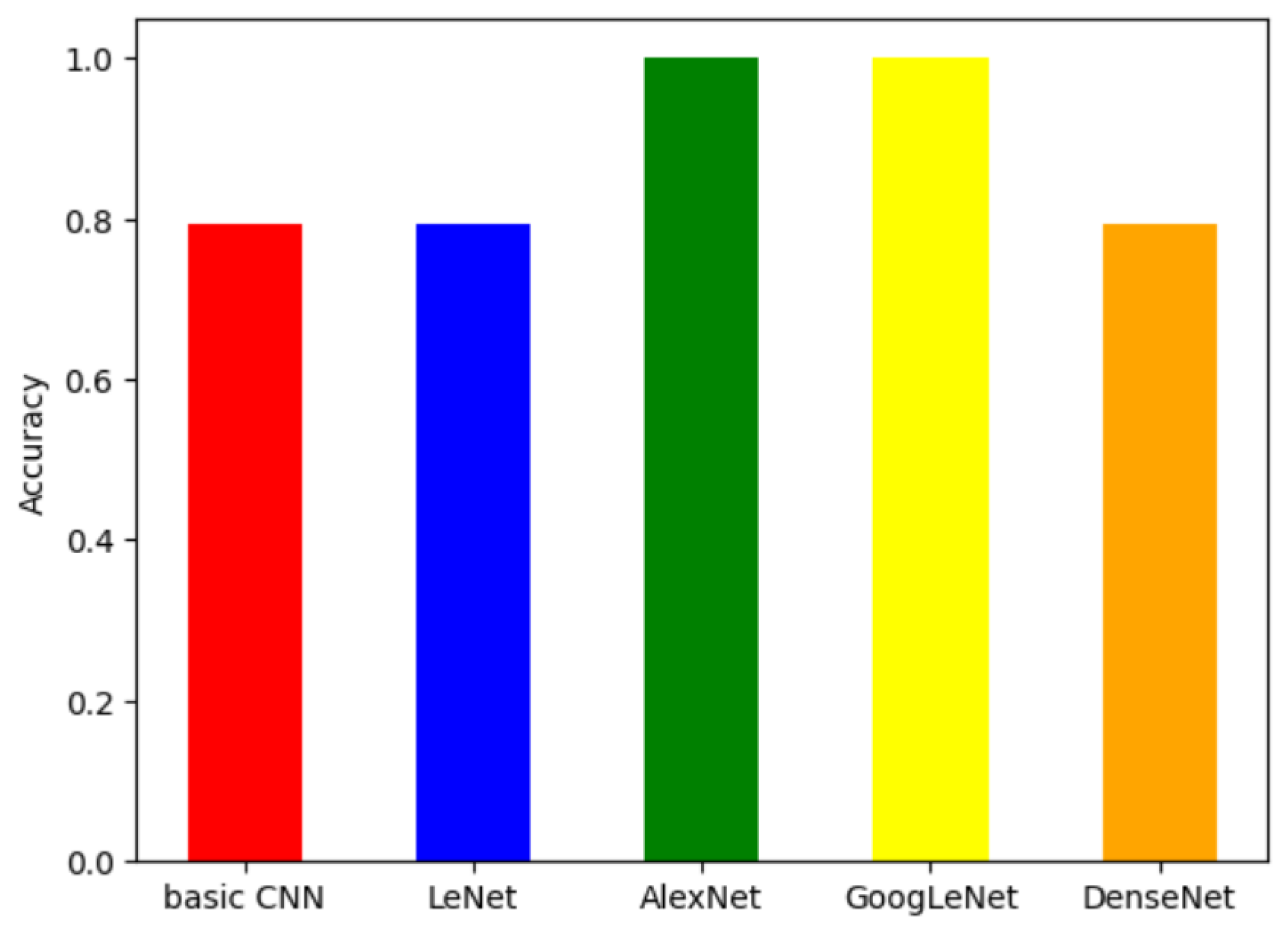
To reduce task complexity, we next performed binary classification between two selected families (VB.AT and Wintrim.BX). As shown in Figure 3, GoogLeNet and AlexNet achieved perfect classification, while the basic CNN, LeNet, and DenseNet reached around 80% accuracy. This suggests that deeper architectures may be more effective when the classification scope is constrained.

We then introduced image perturbations to assess robustness in the two-family setting. Figure 4 shows that even minimal salting (0.01–1%) led to sharp accuracy drops for LeNet and DenseNet, falling to nearly 50%. This indicates that these models rely heavily on specific local patterns that are easily disrupted. Interestingly, the basic CNN displayed counterintuitive behavior: its accuracy improved with salted images compared to clean ones, likely because the perturbations reduced distributional mismatch between training and test sets. However, this also revealed poor generalization to clean data, with the model overfitting to particular low-level structures.

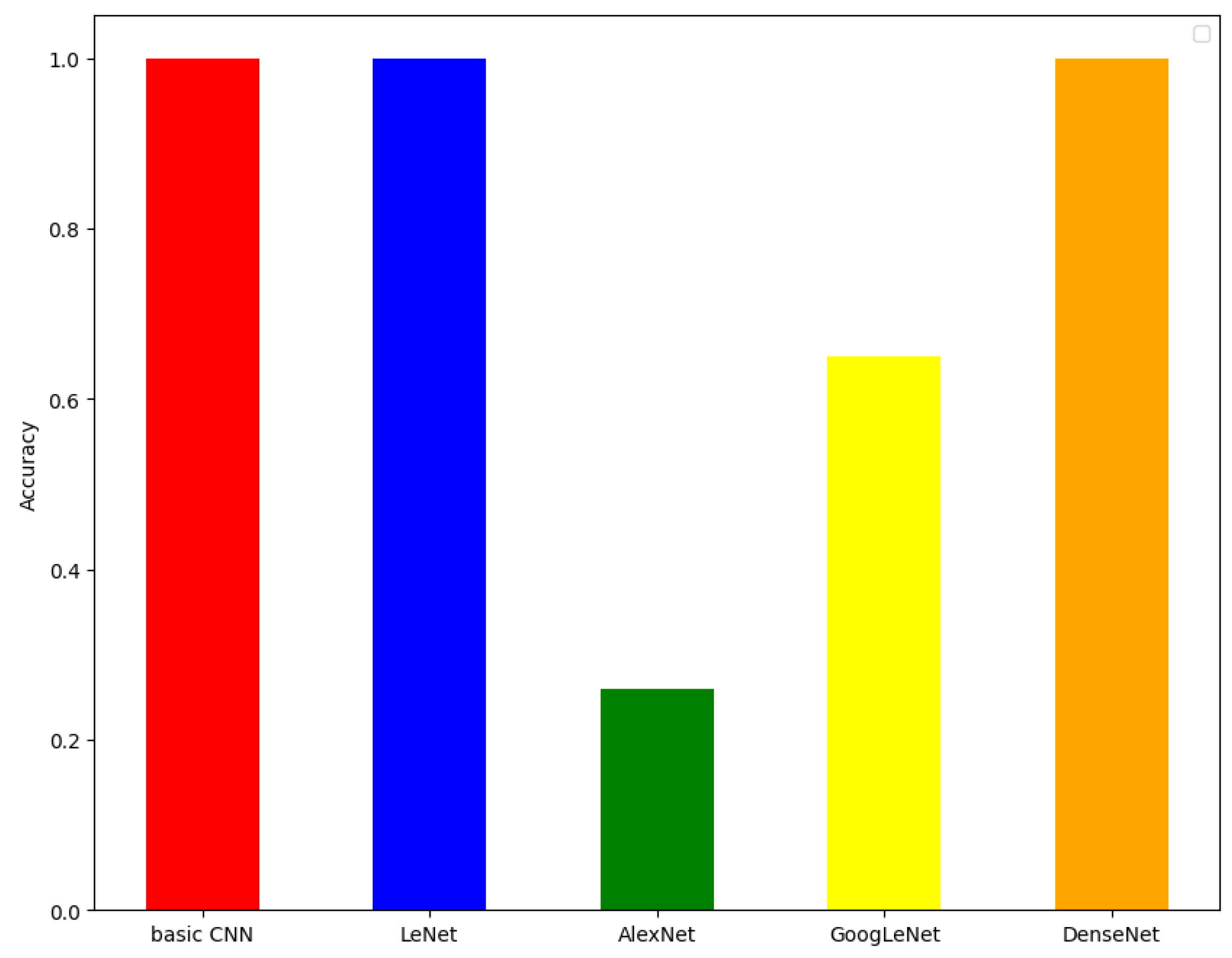
Finally, we evaluated the models on a binary classification task distinguishing between malware (from the Allaple.A family) and a diverse set of benign files. The results in Figure 5 show that the basic CNN, LeNet, and DenseNet achieved near-perfect accuracy on unseen benign samples, demonstrating strong generalization to clean, unaltered data. By contrast, GoogLeNet and AlexNet performed poorly, failing to consistently separate benign from malicious inputs, with accuracies below 70% and 30%, respectively.

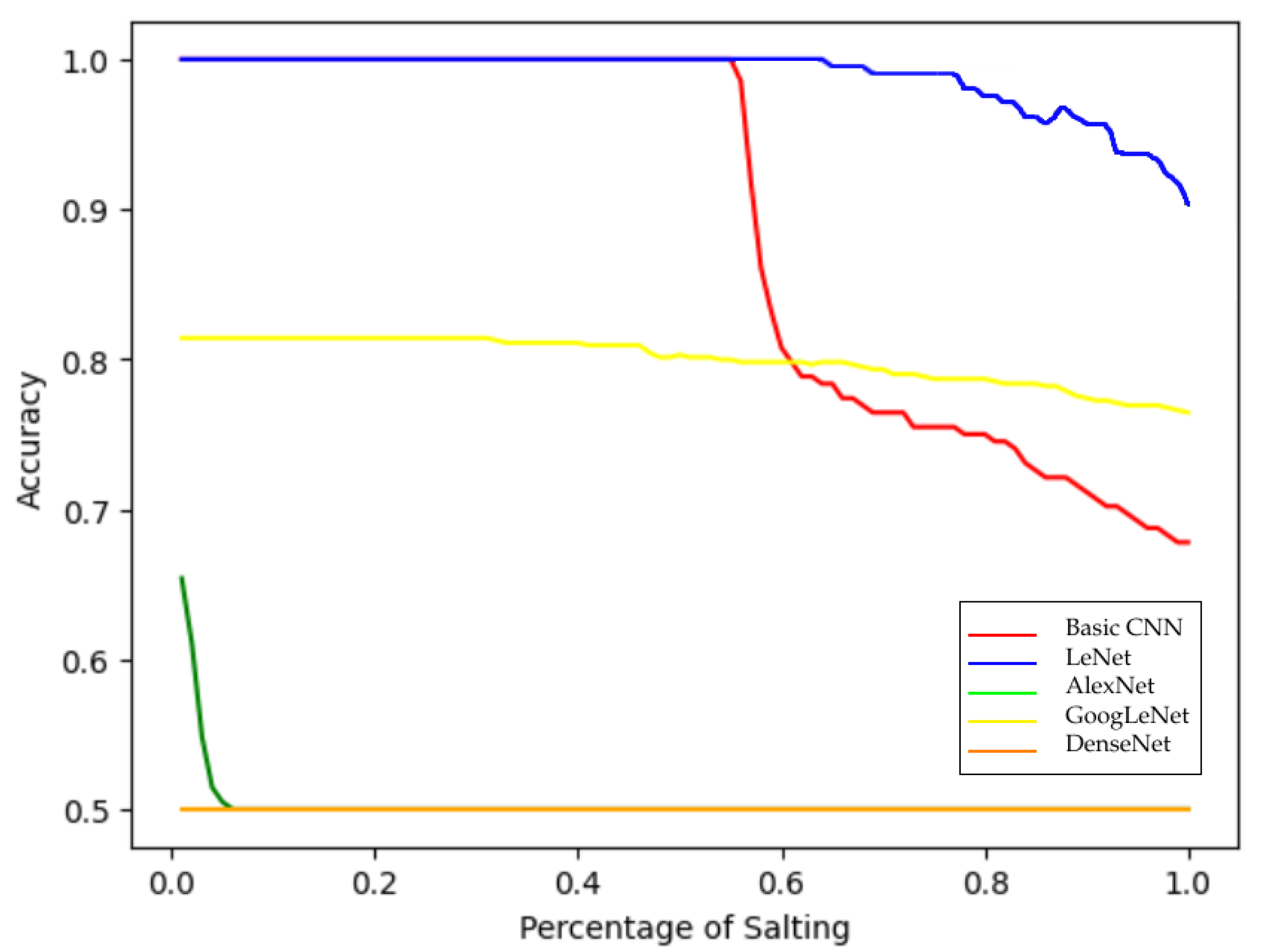
When salting was applied in this malware-versus-benign setting (Figure 6), vulnerabilities across all models became apparent. Basic CNN and LeNet initially performed perfectly but degraded steadily as salting increased. AlexNet and GoogLeNet, which already underperformed on clean data, showed further declines, converging toward random guessing at 50% accuracy. DenseNet, in contrast, misclassified almost all salted malware images as benign, starting at 50% accuracy even with 0.01% salting. Collectively, these results highlight a key weakness: CNN-based malware classifiers are highly susceptible to even minimal perturbations, undermining their reliability in adversarial or noisy environments.

5.3. Merged Dataset Results

The following results are from the merged dataset (Malimg and Virusshare).

In Figure 7, we see the results for the malware family classification. The best performance is GoogLeNet, which is $87\%$, All models other than AlexNet, which has an under $30\%$ accuracy, perform better than $70\%$, demonstrating decent performance in classifying malware images into families. However, the best accuracy is about a $10\%$ drop from that of the Malimg dataset only, likely due to the presence of many minority classes in the merged dataset.

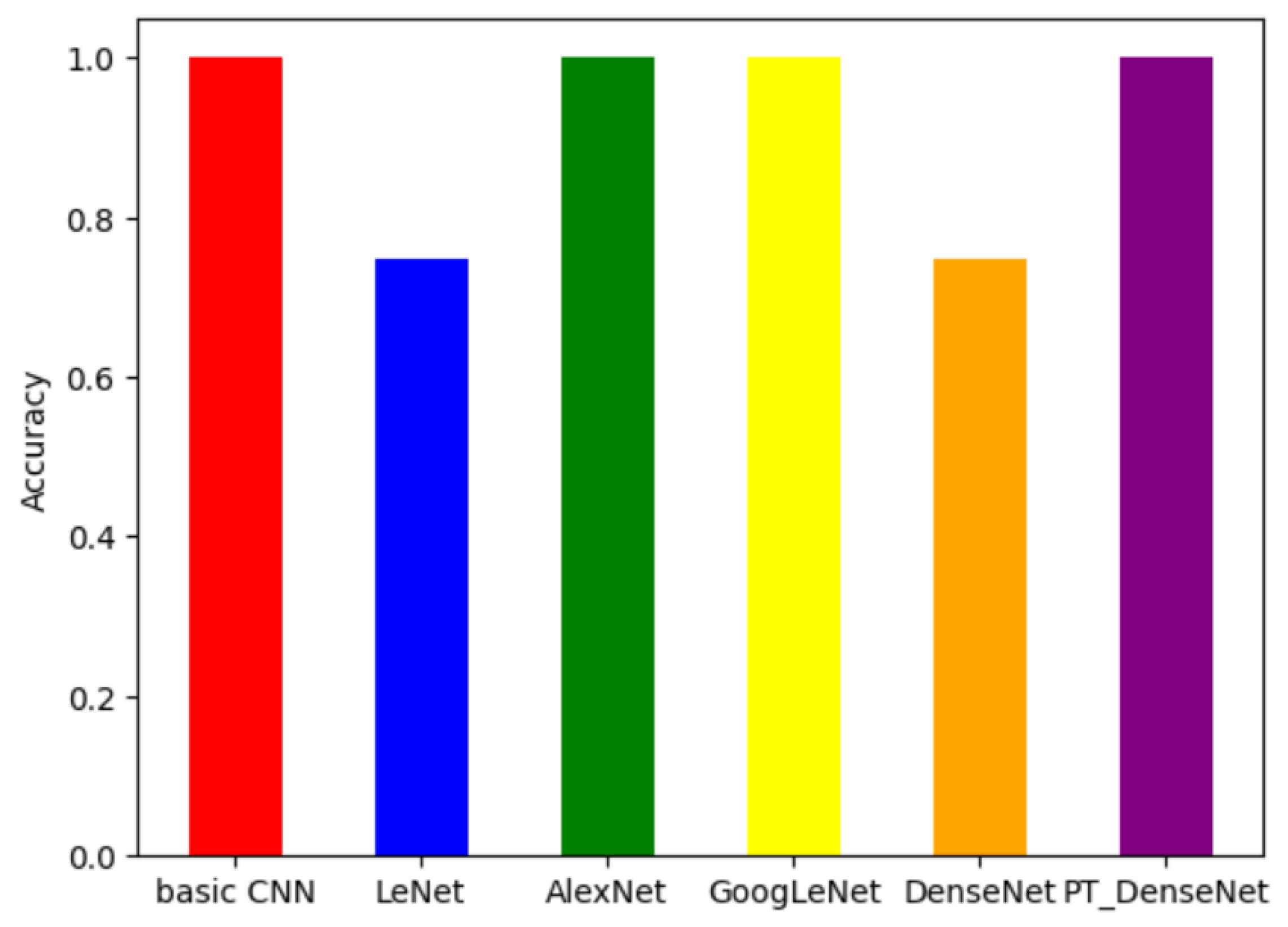
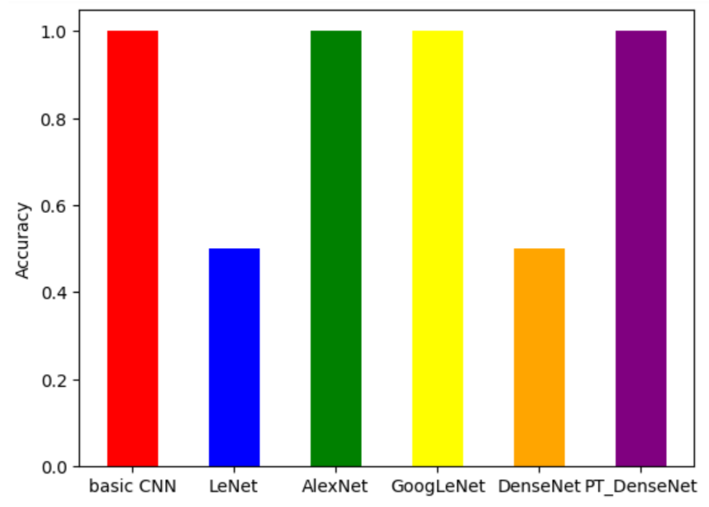
We see the accuracies of each model when trained on the same two malware families, VB.AT and Wintrim.BX in Figure 8. Basic CNN, AlexNet, GoogLeNet, and pretrained DenseNet are able to perfectly classify all images into the family. LeNet and DenseNet have an accuracy of around $73\%$, showing a moderate ability to classify images from these two families.

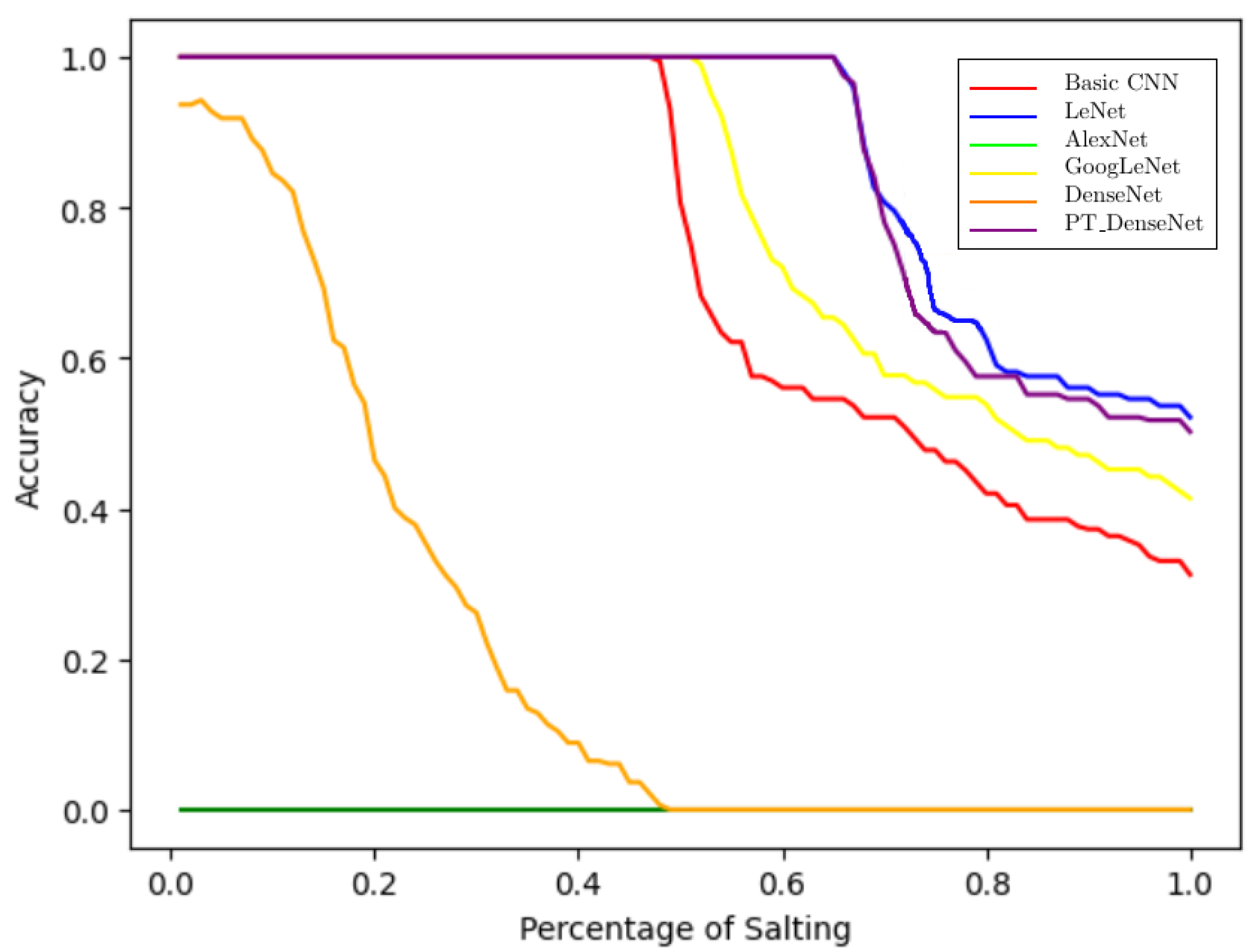
In Figure 9, we see the accuracy of each model when tested on the salted images, with salting between $0.01\%$ and $1\%$. Once again, the accuracies stayed the same throughout the salting. The accuracies of LeNet and DenseNet decreased to $50\%$, showing the confusion of these models caused by image salting, whereas the rest of the models retained their perfect accuracy in the salting experiments as well.

In Figure 10, we see the accuracies of the malware (Allaple.A family) vs. benign experiment when the models are tested on unsalted benign images set aside for testing. All the models show perfect accuracy here, being able to correctly classify the benign images as benign and not malware.

The accuracy of each model when evaluated on the salted images, with salting between $0.01\%$ and $1\%$, are depicted in Figure 11. AlexNet has an accuracy of 0 throughout, indicating that it is completely confused by the salting. It is not possible for AlexNet to always predict an image as benign as that would have led to a $50\%$ accuracy. DenseNet’s accuracy starts just below 1, dropping the fastest as salting increases. Each of the other models start at a perfect accuracy, but they drop and seem to approach 0 as salting increases. Again, the huge effect of slight salting on the CNN models’ performance demonstrates a weakness of CNN models for malware detection.

The evaluation of F1 score, precision, and recall in the merged malware-benign salting experiments reveals patterns that closely parallel the accuracy results. A summary is provided in

Table 6. Comparison of CNN architectures on precision, recall, and F1 score under salting perturbations.

Model	Precision	Recall	F1 Score
Basic CNN	92.55%	81.50%	87.67%
LeNet	94.69%	81.82%	87.89%
AlexNet	0.00%	0.00%	–
GoogLeNet	95.14%	81.34%	87.70%
DenseNet	84.67%	72.61%	78.18%
Pretrained DenseNet	88.44%	80.03%	84.03%

. Similar to the accuracy trends under perturbation, the models consistently exhibited sensitivity to even minimal changes introduced by salting, with performance declining in step with the accuracy curves. This alignment indicates that the observed vulnerabilities are not confined to a single evaluation metric but instead reflect a broader limitation in the models’ robustness. These findings reinforce the conclusion that CNN-based malware classifiers, although effective under clean conditions, remain highly susceptible to small-scale adversarial perturbations in real-world scenarios.

5.4. Different Cropping Rectangles Experiment

Hyperparameter tuning was performed on the merged data set to ensure that the pre-processing steps were performed optimally to foster the best accuracy possible from the models. This involved testing different cropping rectangles. A cropping rectangle is the portion of the image that is retained after the cropping, thus being the only part of each image fed into the model. Each cropping rectangle is a tuple of length 4 formatted in the form $(x_1, y_1, x_2, y_2)$, where $(x_1, y_1)$ is the bottom left corner of the rectangle and $(x_2, y_2)$ is the upper right corner of the rectangle. $(0, 0)$ (the origin) is the bottom left corner of the image. Various cropping rectangles—of sizes 100 by 100, 224 by 224, and 300 by 300—were subject to experiments. Due to the images being of different size, there was no definitive right coordinate of the images. Thus, to enforce consistency, each cropping rectangle size began with the bottom left corner of each rectangle being the origin (bottom left corner of each image). Pretrained DenseNet works only on images of size 224 by 224 pixels, thus the results for all other cropping rectangles are not applicable.

The results of the experiment involving various cropping rectangles are displayed in

Table 7. Accuracy for Basic CNN, LeNet, and AlexNet across cropping configurations.

Crop Size	Rectangle	Basic CNN	LeNet	AlexNet
100 × 100	(0, 0, 100, 100)	82.61%	84.03%	79.18%
	(100, 100, 200, 200)	72.86%	74.55%	45.03%
	(200, 200, 300, 300)	69.38%	71.08%	46.22%
	(300, 300, 400, 400)	48.88%	50.25%	44.71%
	(400, 400, 500, 500)	44.07%	43.25%	34.28%
	(500, 500, 600, 600)	41.10%	36.29%	36.84%
	(600, 600, 700, 700)	39.04%	37.03%	34.37%
	(700, 700, 800, 800)	29.70%	29.79%	29.79%
	(800, 800, 900, 900)	27.46%	27.19%	27.46%
	(900, 900, 1000, 1000)	27.46%	27.19%	27.46%
224 × 224	(0, 0, 224, 224)	82.28%	83.28%	26.91%
	(224, 224, 448, 448)	73.27%	59.59%	56.25%
	(448, 448, 672, 672)	43.62%	37.89%	39.45%
	(672, 672, 896, 896)	38.26%	37.25%	37.80%
300 × 300	(0, 0, 300, 300)	67.14%	62.06%	79.95%
	(300, 300, 600, 600)	49.89%	42.11%	43.98%
	(600, 600, 900, 900)	38.67%	36.89%	38.12%

and

Table 8. Accuracy for GoogLeNet, DenseNet, and Pretrained DenseNet across cropping configurations.

Crop Size	Rectangle	GoogLeNet	DenseNet	Pretrained DenseNet
100 × 100	(0, 0, 100, 100)	79.47%	84.03%	N/A
	(100, 100, 200, 200)	64.63%	42.75%	N/A
	(200, 200, 300, 300)	66.91%	49.29%	N/A
	(300, 300, 400, 400)	40.39%	49.29%	N/A
	(400, 400, 500, 500)	42.72%	42.84%	N/A
	(500, 500, 600, 600)	38.44%	40.18%	N/A
	(600, 600, 700, 700)	35.32%	37.25%	N/A
	(700, 700, 800, 800)	28.37%	29.79%	N/A
	(800, 800, 900, 900)	26.28%	0.05%	N/A
	(900, 900, 1000, 1000)	26.28%	0.05%	N/A
224 × 224	(0, 0, 224, 224)	87.18%	75.29%	82.63%
	(224, 224, 448, 448)	71.47%	68.51%	49.51%
	(448, 448, 672, 672)	42.99%	31.76%	43.90%
	(672, 672, 896, 896)	36.42%	36.98%	13.02%
300 × 300	(0, 0, 300, 300)	83.83%	39.22%	N/A
	(300, 300, 600, 600)	51.01%	18.67%	N/A
	(600, 600, 900, 900)	36.10%	37.03%	N/A

Note: N/A values indicate that the model does not support those crop sizes due to its fixed input size of 224 × 224.

. These findings reveal a consistent trend, with few exceptions, where models achieve higher classification accuracy when provided with image data from the bottom-left region compared to the top-right. This suggests that the bottom-left portion contains more discriminative features tied to the malware’s family. One plausible explanation is rooted in the structure of malware binaries: when converted to grayscale images via rasterization (typically in a row-major format), the bytes near the end of the file are mapped to the lower image regions. Since many malware samples embed or append their payloads toward the end of the binary, these critical sections are likely to appear visually in the bottom-left. While this region may not represent the entire payload, it often captures enough distinct patterns or signature-bearing code fragments to significantly influence classification. Therefore, these results indicate that malware family classification techniques should strategically emphasize the bottom-left quadrant of the image, where semantically rich information is often concentrated, rather than relying uniformly on all image regions.

These spatial patterns interact with model architecture in important ways. All models in this study underwent systematic hyperparameter tuning, so the observed disparities in performance reflect genuine architectural differences rather than under-optimization. AlexNet’s relatively poor performance on multiclass classification tasks may arise from its large parameter count and early fully connected layers, which make it prone to overfitting and poorly suited to compact malware images that lack the hierarchical textures typical of natural images. The basic CNN, with its shallow design and reliance on broader low-level features, sometimes improved under salted conditions, likely because its coarse feature extraction made it less sensitive to localized perturbations. More advanced architectures showed clearer benefits: GoogLeNet, with its inception modules that capture multi-scale features, was particularly effective at binary family classification, suggesting that combining fine- and coarse-grained patterns is advantageous for distinguishing between structurally similar malware families. DenseNet benefited from its dense connectivity, which promotes feature reuse and gradient flow, but this same property appears to increase vulnerability to pixel-level perturbations, as even small disruptions propagate widely through the network. Pretrained DenseNet, while powerful, suffered from a mismatch between its ImageNet-learned priors and the grayscale, rasterized malware domain, limiting its transferability.

Taken together, these observations suggest that architectural suitability for malware image classification depends not only on depth but also on how each design balances granularity, robustness, and feature integration. Future work should explore models that combine the resilience of shallow architectures with the discriminative power of deeper networks, or develop malware-specific architectural innovations that explicitly account for spatial biases and adversarial fragility.

6. Discussion and Future Work

The experiments presented in this study highlight both the promise and fragility of CNN-based malware image classifiers. Across tasks, lightweight models such as LeNet and basic CNNs demonstrated that high accuracy is achievable without large computational overhead, suggesting feasibility for deployment in resource-constrained environments. However, the salting experiments exposed a major vulnerability: even minimal perturbations (<1%) were sufficient to erode classification performance, underscoring the susceptibility of these models to adversarial manipulation. More complex obfuscation strategies such as packing, encryption, or polymorphism would likely exacerbate these weaknesses, raising concerns for real-world reliability.

The merged dataset results provided further insight. While family classification became more difficult, likely due to class imbalance, binary classification robustness improved. This suggests that larger, more heterogeneous datasets can strengthen discriminative features for some tasks but also increase noise when fine-grained distinctions are required.

A critical observation emerged from the cropping experiments. CNNs consistently achieved higher accuracy when trained on bottom-left regions of malware images, with accuracy falling as evaluation shifted toward the top-right. This spatial bias reflects the row-major rasterization process: the bottom-left quadrant often encodes payload-rich sections of binaries, which are semantically more informative for classification. This indicates that classifiers are implicitly leveraging structural properties of the binary-to-image mapping rather than learning uniformly discriminative features across the image.

This work also points to broader directions. Expanding datasets to include more diverse and contemporary malware families will improve generalizability. Exploring encoding schemes beyond row-major rasterization may uncover alternative structural signals. Benchmarking advanced CNN variants, transformers, or hybrid architectures could reveal more resilient feature extractors. Finally, robustness should be tested against stronger adversarial strategies, including gradient-based attacks such as Fast Gradient Sign Method (FGSM), Projected Gradient Descent (PGD), and Carlini & Wagner (CW), and validated in online detection settings where computational efficiency and resilience must coexist.

7. Conclusions

This work evaluated the effectiveness and robustness of CNNs for image-based malware classification across multiple tasks and perturbation scenarios. By rasterizing malware binaries into grayscale images, we demonstrated that CNN architectures are capable of achieving high accuracy in both family-level and malware-versus-benign classification under clean conditions. Lightweight models such as LeNet performed surprisingly well on large-scale multiclass classification, while deeper networks like GoogLeNet excelled in constrained binary settings. These findings confirm that malware images contain discriminative patterns that can be effectively captured by deep learning.

At the same time, our experiments revealed significant limitations in robustness. Even minimal image salting, as low as 0.01% perturbation, caused sharp drops in accuracy for many models, with DenseNet in particular misclassifying nearly all salted malware as benign. Although some architectures (e.g., basic CNN) showed counterintuitive improvements under perturbation, this reflected poor generalization rather than genuine resilience. Similarly, cropping experiments highlighted spatial biases in malware images, with the bottom-left quadrant containing disproportionately informative features likely tied to appended payload structures. These results underscore that CNN-based malware classifiers, while promising in clean laboratory conditions, remain fragile under realistic adversarial or noisy scenarios.

Overall, this study highlights both the potential and the vulnerability of CNNs for malware image classification. The observed performance variations across architectures suggest that robustness depends not only on model depth but also on how features are integrated and propagated. Future research should pursue three directions: (i) developing architectures tailored to the structural properties of malware binaries, (ii) incorporating adversarial training or perturbation-aware regularization to improve resilience, and (iii) exploring hybrid approaches that combine image-based analysis with complementary static or dynamic features. Addressing these challenges will be essential for advancing malware classification systems from proof-of-concept experiments toward deployment in adversarial real-world environments.